Download to read offline


![4 COORDINATE SYSTEMS ON A LINE [CHAP. 1
SolvedProblems
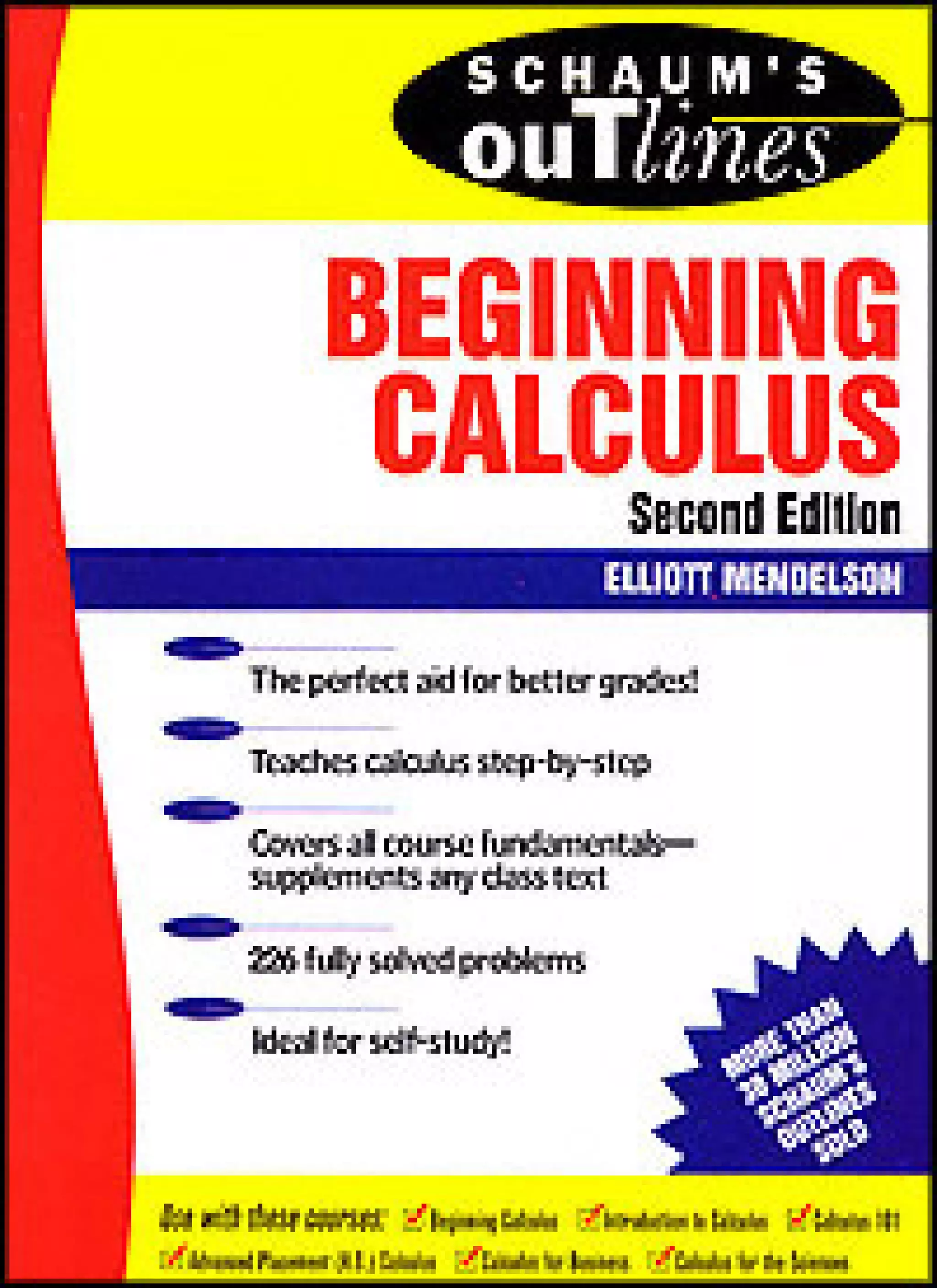
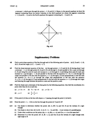
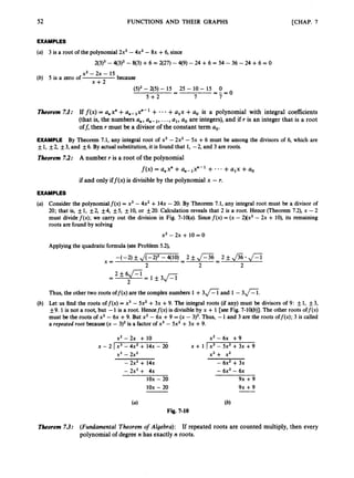
1.1 Recalling that &always denotes the nonnegatiue square root of U, (a)evaluate f l ;
(b)evalu-
ate ,/m;
(c) show that ,
/
? = Ix I. (d)Why isn’t the formula p=
x always true?
(a)f l =
Jd = 3.
(d) By part (c),,
/
? = Ix I, but Ix I = x is false when x < 0. For example, ,
/
- = fi = 3 # -3.
(b)4- = fi = 3. (c) By (1.4),x2 = Ix 1’; hence, since Ix I2 0, = Ix I.
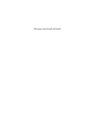
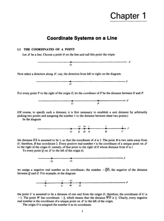
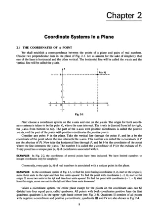
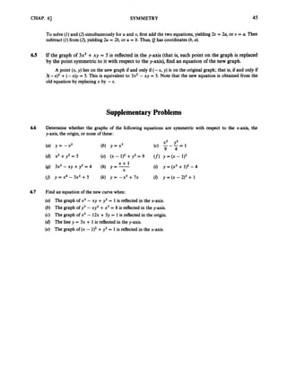
1.2 Solve Ix +3 I 5 5; that is, find all values of x for which the given relation holds.
By (1.8),Ix +31 5 5 if and only if -5 5 x +3 5 5.Subtracting 3, -8 5 x 5 2.
I 1 1
I 1 1
-8 0 2
1.3 Solve I3x +2 I < 1.
By (1.9),I3x +2 I < 1 is equivalent to -1 < 3x +2 < 1. Subtracting 2, we obtain the equivalent rela-
tion -3 < 3x < -1. This is equivalent, upon division by 3,to -1 < x < -3.
I 1 b
- 1 -113 0
1.4 Solve 15 - 3x I<2.
By (1.9), -2 < 5 - 3x < 2
.Subtracting 5, -7 < -3x < -3.Dividing by -3,; > x > 1.
~ ~ ~
ALGEBRA REVIEW Multiplying or dividing both sides of an inequality by a negative number reuerses the
inequality: if U < b and c < 0, then uc > bc.
To see this, notice that a < b implies b - a > 0. Hence, (b - U)C < 0, since the product of a positive
number and a negative number is negative. So bc - ac < 0, or bc < ac.
1.5 Solve
-
I 1 1 1
7
I I 1 . b
0 1 2 3
x + 4 < 2
x - 3
We cannot simply multiply both sides by x - 3,because we do not know whether x - 3 is positive or
negative.
Case 1: x - 3 > 0
.Multiplying (1) by this positive quantity preserves the inequality:
x +4 < 2~ - 6
4 < x - 6 [subtract x]
10 < x [add 61
Thus, if x > 3,(1)holds if and only if x > 10.
Case 2: x - 3 < 0.Multiplying (1) by this negative quantity reverses the inequality:
x +4 > 2~ - 6
4 > x - 6
10 > x [add 61
[subtract x]](https://image.slidesharecdn.com/problemscalculus-221128025033-038ef06f/85/problems-calculus-pdf-17-320.jpg)
![6
1.10
1.11
1.12
1.13
1.14
1.15
1.16
1.17
1.18
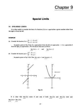
1.19
1.20
1.21
1.22
[CHAP. 1
COORDINATE SYSTEMS ON A LINE
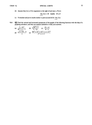
(a) Solve I2x +3I = 4. (b) Solve I5x - 7 I = 1. (c) m Solve part (a) by graphing y, = (2x+ 3I and
y, = 4. Similarly for part (b).
Solve: (a) Ix - 11< 1 (b) 13x + 51 14 (c) I X +41 > 2
(4 1 2 ~ - 5 1 2 3 (e) I x 2 - 1 0 ( ~ 6 (f) 1?+31<1
X
(9)[H3 Check your answers to parts (a)-(f) by graphing.
(4 11+:1>2 (e) 1 < 3 - 2 x < 5 (f) 3 1 2 x + 1 < 4
(9)IE3 Check your answers to parts (a)-(f) by graphing.
Solve: (a) x(x +2) > 0 (b) (X - 1)(x +4) < 0 (c) X’ - 6~ + 5 > 0
(4 x 2 + 7 x - 8 < 0 (e) x2 < 3x + 4 (f)x(x - 1Nx + 1) > 0
(9) ( 2 ~
+ 1)(x - 3 ) ( ~
+7) < 0
(h) Check your answers to parts (a)-@) by graphing.
[Hints: In part (c),factor; in part (f),
use the method of Problem 1.8.1
Show that if b # 0, then - = -
1;l It;
Prove: (a) 1a21= lalZ (b)
Solve: (a) 12x - 31 = Ix +21
[Hint: Use ( I 4.1
a3I = Ia l3 (c) Generalize the results of parts (a)and (b).
(b) 17x-51=13x+41 (c) 2x- 1 = I x + 7 )
(d) Check your answers to parts (a)-@)by graphing.
Solve: (a) 12x - 31 < Ix + 21
(b) I3x - 2 I 5 Ix - 1I
[Hint: Consider the threecasesx 2 3, -2 I
x < 3,x < -2.1
(c) mCheck your solutions to parts (a)and (b) by graphing.
(a) Prove: [ a- bl 2 Ilal - Ibl I.
and Ibl I [ a- bl +[al.]
(b) Prove: la - 61 I lal + 161.
[Hint: Use the triangle inequality to prove that lal 5 l a - bl +lbl
Determine whether f l =
a
’ holds for all real numbers a.
Does f l < always imply that a < b?
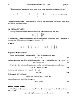
Let 0,
I , A, B, C, D be points on a line, with respective coordinates0, 1,4, -1,3, and -4. Draw a diagram
showing these points and find: m,
AI,m,z
,
a+m,ID, +z
,
E.
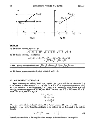
Let A and B be points with coordinates a and b. Find b if: (a) a = 7, B is to the right of A, and
Ib - a1 = 3; (b) a = -1, Bis to the left of A, and Ib - a / = 4; (c)a = -2, b < 0, and Ib - a1 = 3.](https://image.slidesharecdn.com/problemscalculus-221128025033-038ef06f/85/problems-calculus-pdf-19-320.jpg)
![CHAP. 11 COORDINATE SYSTEMS ON A LINE
1.23 Prove: (a) a < b is equivalent to a +c < b +c.
7
ALGEBRA a < b means that b - a is positive. The sum and the product of two positive numbers are posi-
tive, the product of two negative numbers is positive, and the product of a positive and a negative number
is negative.
a b
(b) If 0 < c, then a < b is equivalent to ac < bc and to - < -.
c c
1.24 Prove (1.6).[Hint: Consider three cases: (a)A, and A, on the positive x-axis or at the origin; (b)A, and A,
on the negative x-axis or at the origin; (c) A, and A, on opposite sides of the origin.]](https://image.slidesharecdn.com/problemscalculus-221128025033-038ef06f/85/problems-calculus-pdf-20-320.jpg)
![CHAP. 23
4 Y
(-2.4)
T
4
I
4
4 -
(-2.3) 3 - 0 (3.3)
2 - 0 (2.2) (5.2) +
I
(3.0) 1
- I + 1 - 1 -
I -
(-4,I)
1 1 1 1 1 I A I 1
-4 - 3 - 2 - 1 0 I 2 3 4 5 x %+*
‘ - 2 ,
4
0 (-3. -2) -2(C (0, -2)
-3 - 0 (4, -3) (-1,-3) 1 -3
COORDINATE SYSTEMS IN A PLANE
4 Y
4 -
3 -
2 - 9 (3*2)
1 -
3 4 5 x
-
9
11 3 -
(-1.2) 0 2
(-. +)
I 1 I
-3 -2 - 1 0
0 (-3,-1) -1
4 Y
I
(+*+)
-
I ’ 0 (2.1)
I 1 I
1 2 3
-
Fig. 2-4
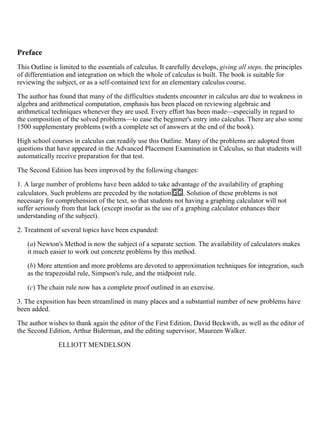
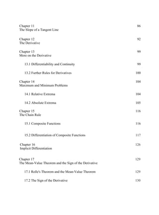
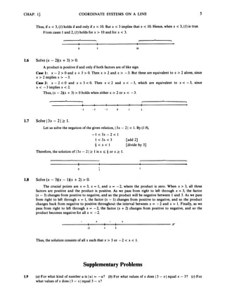
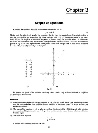
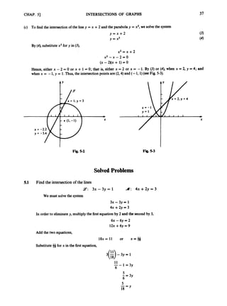
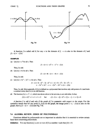
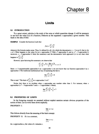
The points having coordinates of the form (0, b) are precisely the points on the y-axis. The points
If a coordinate system is given, it is customary to refer to the point with coordinates (a, b) simply as
having coordinates (a,0)are the points on the x-axis.
“the point (a,b).”Thus, one might say: “The point (1,O) lies on the x-axis.”
2.2 THE DISTANCE FORMULA
Let P1and P, be points with coordinates (x,, y,) and (x,, y,) in a given coordinate system (Fig.
2-5). We wish to find a formula for the distancePIP2.
Let R be the point where the vertical line through P, intersects the horizontal line through P,.
Clearly, the x-coordinate of R is x2,the same as that of P,;and the y-coordinate of R is y,, the same as
that of P,.By the Pythagorean theorem,
-
= Fp2
+P,R2
Now if A, .and A, are the projections of P, and P2 on the x-axis, the segments P,R and A,&
are opposite sides of a rectangle. Hence, P,R = A,& But A,A2 = Ix, -x, I by (1.6). Thus,
- -
= Ix, - x2I. Similarly,P,R = Iy1 - y, I. Consequently,
PlP,* = Ix1 - x2 1, + IY l - Y, 1
, = (x, - x2), +011 - Y,),
PlP, = Jbl -x2I2 +b
1- Y,),
whence
[Equation (2.1) is called the distance formula.] The reader should check that this formula also holds
when P,and P, lie on the same horizontal line or on the same vertical line.
(2.1)](https://image.slidesharecdn.com/problemscalculus-221128025033-038ef06f/85/problems-calculus-pdf-22-320.jpg)
![CHAP. 21 COORDINATE SYSTEMS IN A PLANE 11
EXAMPLES
(a) The midpoint of the segment connecting(1, 7)and (3, 5) is (F,
y)
= (2,6).
-
(b) The point halfway between (-2, 5) and (3, 3)is (*, =)
-
- (i,4).
2 2
Solved Problems
2.1 Determine whether the triangle with vertices A( -1,2),B
(
4
,7), C(-3,6) is isosceles.
-
AB = J(-1 - 4)2 +(2 - 7)2= J(-5)2 + ( - 5 ) 2 = ,/ET% = Jso
AC = J[-1 - (-3)12 +(2 - 6)2= Jw'
= JGZ = JZ
BC = J[4 - (-3)]' +(7 - 6)2= J7T+1z = JZGT = Jso
-
-
Since AB = E
,
the triangle is isosceles.
2.2 Determine whether the triangle with vertices A( -5, -3),B( -7, 3), C(2,6)is a right triangle.
Use (2.2)to find the squares of the sides,
-
AB2 = ( - 5 +7)2+(-3 - 3)2= 22 +(-6)2 = 4 + 36 = 40
BC2 = (-7 - 2)2+(3 - 6)2= 81 +9 = 90
AC2 = (-5 - 2)2+(-3 - 6)2= 49 + 81 = 130
-
-
SinceAB2 +m2= E2,
AABC is a right triangle with right angle at B.
GEOMETRY The converse of the Pythagorean theorem is also true: If x2
= AB2 +m2in AABC, then
<ABC is a right angle.
2
.
3 Prove by use of coordinates that the midpoint of the hypotenuse of a right triangle is equidistant
from the three vertices.
Let the origin of a coordinate system be located at the right angle C; let the positive x-axis contain leg
CA and the positive y-axis leg CB [see Fig. 2-7(a)].
Vertex A has coordinates (b, 0),where b = CA; and vertex B has coordinates (0, a), where a = E.
Let
M be the midpoint of the hypotenuse. By the midpoint formulas (2.2),the coordinates of M are (b/2, a/2).
-
(a)
Fig. 2-7](https://image.slidesharecdn.com/problemscalculus-221128025033-038ef06f/85/problems-calculus-pdf-24-320.jpg)
![12 COORDINATE SYSTEMS IN A PLANE
Now by the Pythagorean theorem,
and by the distance formula (24,
[CHAP. 2
ALGEBRA For any positive numbers U, U,
- -
Hence, MA = MC. [For a simpler, geometrical proof, see Fig. 2-7(b);MD and BC are parallel.]
Supplementary Problems
2.4 In Fig. 2-8, find the coordinates of points A, B,C, D, E, and F.
2.5 Draw a coordinate system and mark the points having the following coordinates: (1, -l), (4, 4), (-2, -2),
(3, -31, (0,2),(2,0),(-4, 1).
2.6 Find the distance between the points: (a) (2, 3) and (2, 8); (b) (3, 1) and (3, -4); (c) (4, 1) and (2, 1);
(4(-3,4) and (54).
2.7 Draw the triangle with vertices A(4, 7), B(4, -3), and C
(-1,7) and find its area.
2.8 If (-2, -2), (-2,4), and (3, -2) are three vertices of a rectangle, find the fourth vertex.
e F
E
Fig. 2-8](https://image.slidesharecdn.com/problemscalculus-221128025033-038ef06f/85/problems-calculus-pdf-25-320.jpg)
![CHAP. 3) GRAPHS OF EQUATIONS 17
0
0
0
0
0
0
0
0
on completing the squares; that is, replacing the quantities x2 +Ax and y2 +By by the equal quantities
A2 and ( y + : ) ’ - ~
B2
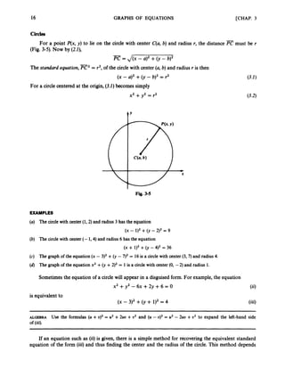
EXAMPLE Let us find the graph of the equation
x 2 + y 2 + 4 x - 2 y + 1 = o
( x + 2 ) 2 - 4 + ( y - 1 ) 2 - 1 + 1 = o
(x +2)2 +(y - 1)2= 4
Completing the squares, replace x2 +4x by (x +2)2- 4 and y2 - 2y by (y - 1)2- 1,
This is the equation of a circle with center (- 2, 1)and radius 2.
Solved Problems
3
.
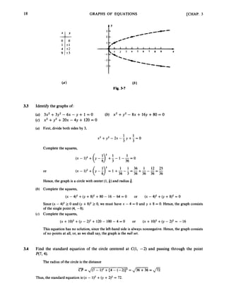
1 Find the graph of: (a)the equation x = 2; (b) the equation y = -3.
(a) The points satisfying the equation x = 2 are of the form (2, y), where y can be any number. These
points form a vertical line [Fig. 3-6(a)].
(6) The points satisfying y = -3 are of the form (x, -3), where x is any number. These points form a
horizontal line [Fig. 3-6(6)].
I
Fig. 3-6
3
.
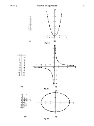
2 Find the graph of the equation x = y2.
2
:F
...... ..............
- 3 t
Plotting several points suggests the curve shown in Fig. 3-7. This curve is a parabola, which may be
obtained from the graph of y = x2(Fig. 3-2) by switching the x- and y-coordinates.](https://image.slidesharecdn.com/problemscalculus-221128025033-038ef06f/85/problems-calculus-pdf-30-320.jpg)
![CHAP. 31 GRAPHS OF EQUATIONS 19
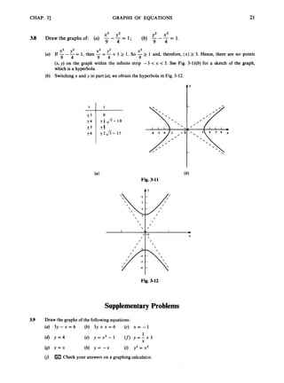
3.5 Find the graphs of: (a)y = x2 +2; (b)y = x2 - 2;(c) y = (x - 2)2;(6)Y = (x +2)2.
The graph of y = x2 +2 is obtained from the graph of y = x2 (Fig. 3-2)by raising each point two units
in the vertical direction [see Fig. 3-8(a)].
The graph of y = x2 - 2 is obtained from the graph of y = x2 by lowering each point two units [see
Fig. 3-8(b)].
The graph of y = (x - 2)2 is obtained from the graph of y = x2 by moving every point of the latter
graph two units to the right [see Fig. 3-8(c)]. To see this, assume (a, b) is on y = (x - 2)2. Then
b = (a - 2)2. Hence, the,point (a - 2, b) satisfies y = x2 and therefore is on the graph of y = x2. But
(a,b) is obtained by moving (a - 2, b) two units to the right.
The graph of y = (x +2)2is obtained from the graph of y = x2 by moving every point two units to the
left [see Fig. 3-8(d)]. The reasoning is as in part (c).
Parts (c) and (d) can be generalized as follows. If c is a positive number, the graph of the equation
/
;c I
F(x - c, y) = 0 is obtained from the graph of F(x, y) = 0 by moving each point of the latter graph c units to
the right. The graph of F(x +c, y) = 0 is obtained from the graph of F(x, y) = 0 by moving each point of
9
3
4
- I
1 1 I ' l l
b
- 3 - 2 0
the latter graph c units to the left.
F L
7,
6 - I
I
I
4 - I
I
5 -
2
: Ii
I - I
- b
I l l 1 1 1
I / 2
1 1 1 1 1
-2 - 1 0
;
I
I
I
I
I
I
I
9
I
/
/
/
#
1 -
1 1 1 1 1 ,
I 2 X
t
/ 2
I
?
I
;-3
-
1 -
1 1 I J l
-5 -4 -3 -2 - 1 0
I 1 1 1 1
I 2
x
-
i
I
I
t
t t
Fig. 3-8](https://image.slidesharecdn.com/problemscalculus-221128025033-038ef06f/85/problems-calculus-pdf-32-320.jpg)
![20 GRAPHS OF EQUATIONS [CHAP. 3
3
.
6 Find the graphs of: (a)x = 0) - 2)2;(b)x = ( y +2)2.
(a) The graph of x = (y - 2)2 is obtained by raising the graph of x = y2 [Fig. 3-7(b)]by two units [see
Fig. 3-9(a)]. The argument is analogous to that for Problem 3 3 4 .
(b) The graph of x = (y +2)2 is obtained by loweringthe graph of x = y2 two units [see Fig. 3-9(b)].
These two results can be generalized as follows. If c is a positive number, the graph of the equation
F(x,y - c) = 0 is obtained from the graph of F(x, y) = 0 by moving each point of the latter graph c units
vertically upward. The graph of F(x, y +c) = 0 is obtained from the graph of F(x, y) = 0 by moving each
point of the latter graph c units vertically downward.
3
.
7
Fig. 3-9
I 2 3 4
I 1 1 1 +
X
Find the graphs of: (a)y = (x - 3)2 +2; (b)fix - 2) = 1.
(a) By Problems 3.5 and 3.6, the graph is obtained by moving the parabola y = x2 three units to the right
and two units upward [see Fig. 3-1qu)l.
(b) By Problem 3.5,the graph is obtained by moving the hyperbola xy = 1 (Fig. 3-3)two units to the right
[see Fig. 3-1qb)l.
Fig. 3-10](https://image.slidesharecdn.com/problemscalculus-221128025033-038ef06f/85/problems-calculus-pdf-33-320.jpg)
![22
3.10
3.11
3.12
3.13
GRAPHS OF EQUATIONS
On a single diagram, draw the graphs of:
[CHAP. 3
1 1
y = x 2 (b) y = 2x2 (c) y = 3x2 (d) y = j x 2 (e) y = j x 2
Check your answers on a graphing calculator.
Draw the graph of y = (x - 1)2.(Include all points with x = -2, -1, 0, 1, 2, 3, 4.) How is this graph
related to the graph of y = x2? Check on a graphing calculator.
. Check on a graphing calculator.
1
Draw the graph of y = -
x - 1
Draw the graph of y = (x + 1)2. How is this graph related to that of y = x2?[H3 Check on a graphing
calculator.
.
1
Draw the graph of y = -
x + l
Check on a graphing calculator.
Sketch the graphs of the followingequations. Check your answers on a graphing calculator.
(c) x2 - y2 = 1
x2 y2
(a) -+-= 1 (b) 4x2 +y2 = 4
4 9
(4 Y = x 3
[Hint:
Parts (c) and (f) are hyperbolas. Obtain part (e)from part (a).]
Find an equation whose graph consists of all points P(x, y) whose distance from the point F(0, p)
is equal to its distance PQ from the horizontal line y = - p (p is a fixed positive number). (See
Fig. 3-13.)
0
- p I
Fig. 3-13
3.14 Find the standard equations of the circles satisfying the given conditions: (a) center (4, 3), radius 1;
(b) center (- 1, 9, radius fi;(c) center (0, 2), radius 4; (d)center (3, 3), radius 3fi; (e) center (4, -1)
and passing through (2, 3); (f)
center (1,2) and passing through the origin.
3.15 Identify the graphs of the followingequations:
(U)
(c) x2 +y2 +3x - 2y +4 = 0
(e)
X’ +y2- 1 2 ~
+20y + 15 = 0 (b) x2 +y2 +30y +29 = 0
(d) 2x2 + 2y2 - x = 0
x2 +y2 +2x - 2y +2 = O (f)x2 +y2 +6x +4y = 36](https://image.slidesharecdn.com/problemscalculus-221128025033-038ef06f/85/problems-calculus-pdf-35-320.jpg)
![CHAP. 31 GRAPHS OF EQUATIONS 23
3.16
3.17
3.18
3.19
3.20
(a) Problem 3.3 suggests that the graph of the equation x2 +y2 +Dx +Ey +F = 0 is either a circle, a
point, or the null set. Prove this.
(b) Find a condition on the numbers D, E, F which is equivalent to the graph’s being a circle. [Hint:
Completethe squares.]
Find the standard equation of a circle passin through the following points. (a) (3, 8), (9, 6),
and (13, -2); (b) (5, 5), (9, l), and (0, d.
[Hint: Write the equation in the nonstandard
form x2 +y2 +Dx +Ey +F = 0 and then substitute the values of x and y given by the three points. Solve
the three resultingequationsfor D, E, and F.]
For what value@)
of k does the circle (x - k)2 +0,-2k)2 = 10pass through the point (1, l)?
Find the standard equationsof the circles of radius 3 that are tangent to both linesx = 4 and y = 6.
What are the coordinates of the center(s)of the circle@)of radius 5 that pass through the points (- 1,7)and
(
-
2
.
9 6)?](https://image.slidesharecdn.com/problemscalculus-221128025033-038ef06f/85/problems-calculus-pdf-36-320.jpg)
![26 STRAIGHT LINES [CHAP. 4
f’
(4
Fig. 4-3
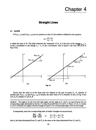
Now let us see how the slope varies with the “steepness” of the line. First let us consider lines with
positive slopes, passing through a fixed point P,(x,, yJ. One such line is shown in Fig. 4-4. Take
another point, P2(x2,y,), on A? such that x2 - x1 = 1. Then, by definition, the slope rn is equal to the
distance RP, .Now as the steepnessof the line increases, RP, increases without limit [see Fig. 4-5(a)J.
Thus, the slope of 9increases from 0 (when 9is horizontal) to +CO (when 9 is vertical). By a similar
construction we can show that as a negatively sloped line becomes steeper and steeper,the slope stead-
ily decreases from 0 (when the line is horizontal) to -CQ (when the line is vertical) [see Fig. 4-5(b)].
- -
t’ Y
Fig. 44](https://image.slidesharecdn.com/problemscalculus-221128025033-038ef06f/85/problems-calculus-pdf-39-320.jpg)
![CHAP. 41 STRAIGHT LINES
4 Y
m = O m = O
27
(a1
Fig. 4-5
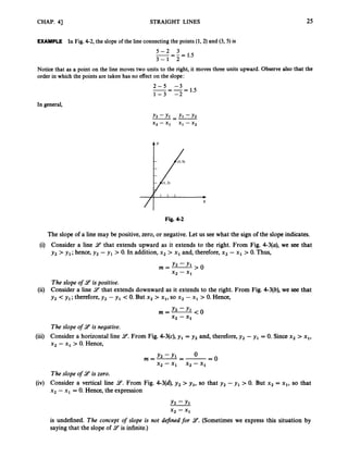
4.2 EQUATIONS OF A LINE
Consider a line 9
’ that passes through the point P,(x,, y,) and has slope rn [Fig. 4-6(a)]. For any
other point P(x,y) on the line, the slopern is, by definition,the ratio of y - y, to x - xl. Hence,
O
n the other hand, if P(x, y) is not on line 9 [Fig. 4-6(b)], then the slope (y -y,)/(x - x,) of the line
PP,is different from the slope rn of 9,so that (4.1)does not hold. Equation (4.1)can be rewritten as
Note that (4.2)is also satisfied by the point (x,, y,). So a point (x, y)is on line 14 if and only if it satisfies
(4.2);that is, 9 is the graph of (4.2).Equation (4.2)is called a point-slope equation of the line 9.
t Y
c
X
t Y
X
EXAMPLES
(U) A point-slope equation of the line going through the point (1,3) with slope 5 is
(b) Let 9 be the line through the points (1,4) and (- 1,2). The slope of 9 is
y -3 = 5(x - 1)
2 1
4 - 2
m=-=-=
1-(-1) 2](https://image.slidesharecdn.com/problemscalculus-221128025033-038ef06f/85/problems-calculus-pdf-40-320.jpg)
![28 STRAIGHT LINES [CHAP. 4
Therefore, two point-slopeequationsof 9 are
Y - 4 - x - 1 and y - 2 = ~ + 1
Equation (4.2) is equivalentto
y-y, =mx-mx, or y=mx+(y, -mx,)
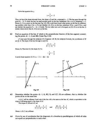
Let b stand for the numbery, - mx,.Then the equation becomes
y = m x + b (4.3)
When x = 0, (4.3) yields the value y = b. Hence, the point (0,b) lies on 9.Thus, b is the y-coordinate of
the point where 9 intersects the y-axis (see Fig. 4-7). The number b is called the y-intercept of 9,and
(4.3)is called the slope-interceptequation of 9.
4 Y
Y
*
X
Fig. 4-7
EXAMPLE Let 14 be the line through points (1,3) and (2, 5). Its slopem is
5 - 3 2
-- - - = 2
2 - 1 1
Its slope-interceptequation must have the form y = 2x +b. Since the point (1, 3) is on line 14,(1,3) must satisfythe
equation
3 = 2(1) +b
So, b = 1, giving y = 2x + 1 as the slope-interceptequation.
An alternativemethod is to write down a point-slopeequation,
whence,
y -3 = 2(x - 1)
y - 3 = 2x -2
y = 2 x + 1
4 3 PARALLEL LINES
Assume that 9,and 9, are parallel, nonvertical lines, and let P, and P, be the points where 2Yl
and 9
, cut the y-axis [see Fig. 4-8(u)]. Let R, be one unit to the right of P,,and R, one unit to the
right of P,. Let Q, and Q2be the intersections of the vertical lines through RI and R2with 2Yl and
Y 2 .
Now AP,RIQ1is congruent to AP, R2Qz.
GEOMETRY U
s
e the ASA (angle-side-angle)congruencetheorem. S R I = SR, since both are right angles,
-
P1R-,=P2R2=1
<P1= %P,,since SP,and <P, are formed by pairs of parallel lines.](https://image.slidesharecdn.com/problemscalculus-221128025033-038ef06f/85/problems-calculus-pdf-41-320.jpg)
![CHAP. 41
A Y
STRAIGHT LINES
t’
29
Fig. 4-8
- -
Hence, RIQl
= R2Q2,
and
- -
slope of Yl = -
RIQ1
-
--
R 2 Q 2-
- slope of 9 2
1 1
Thus, parallel lines have equal slopes.
Conversely,if different lines Yl and Y 2
are not parallel, then their slopes must be different. For if
Yl and 9, meet at the point P [see Fig. 4-8(b)] and if their slopes are the same, then Yl and Y 2
would have to be the same line. Thus, we have proved:
Theorem4.1: Two distinct lines are parallel if and only if their slopes are equal.
EXAMPLE Let us find an equation of the line 9through (3, 2) and parallel to the line A having the equation
3x - y = 2. The line A has slope-intercept equation y = 3x +2. Hence, the slope of A is 3, and the slope of the
parallel line 9also must be 3. The slope-intercept equation of 9 must then be of the form y = 3x +b. Since(3, 2)
lies on 9,2 = 3(3) +b, or b = -7. Thus, the slope-intercept equation of 9is y = 3x - 7. An equivalent equation
is 3x -y = 7.
4.4 PERPENDICULAR LINES
Theorem4.2: Two nonvertical lines are perpendicular if and only if the product of their slopes is -1.
Hence, if the slope of one of the lines’isrn, then the slope of the other line is the negative
reciprocal -l/m.
For a proof, see Problem 4.5.
4.1 Find the slope of the line having the equation 5x - 2y = 4. Draw the line and determine whether
the points (10,23)and (6, 12)are on the line.](https://image.slidesharecdn.com/problemscalculus-221128025033-038ef06f/85/problems-calculus-pdf-42-320.jpg)
![CHAP. 41 STRAIGHT LINES 31
Represent the rhombus as in Fig. 4-11. (How do we know that the x-coordinate of D is U +U?) Then
the slope of diagonal AD is
W
--
w - 0
m, =
u + u - 0 - u + u
and the slope of diagonal BC is
Hence,
w - 0 w
m2=-=-
U - U U - U
W2
m,m2= - - =-
(U: U
) u2 - u2
Since ABDC is a rhombus,AB = E.But AB = U and AC = ,
/
=
. So,
Jm-
= U or u2 +w2 = U ’ or w2 =U’ - u2
Consequently,
w2 u2 - u2
m , m , = m = p - J = - 1
and, by Theorem4.2,lines AD and BC are perpendicular.
t Y C(u.
w ) D(u+ U. w )
Fig. 4-11
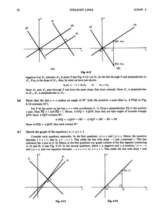
4.5 Prove Theorem 4.2.
Assume that 9,
and 9,
are perpendicular nonvertical lines of respective slopes m, and m, .We shall
show that m1m2 = -1.
Let 1
4
: be the line through the origin 0 and parallel to 9,,
and let 1
4
: be the line through the origin
and parallel to 14, [see Fig. 4-12(a)]. Since 147 is parallel to 14,and 2’;
is parallel to 9,,
the slope of 147
is m, and the slope of 9
:
is m2 (by Theorem 4.1).Also 1
4
: is perpendicular to 9;
since9,
is perpendicu-
lar to 14,. Let R be the point on 9fwith x-coordinate 1, and let Q be the point on 9
3with x-coordinate
1 [see Fig. 4-12(b)]. The slope-interceptequation of 1
4
: is y = mlx, and so the y-coordinate of R ism, since
its x-coordinate is 1.Similarly,the y-coordinateof Q is m, .By the distance formula,
-
OQ = J(1 -0
)
’+(m,-0
)
’ = ,
/
-
OR = ,/(l - O), +(ml- 0
)
’= Jm
-
-
’ QR = &i - i)2 +(mz-ml)2 = ,
/
-
By the Pythagorean theoremfor the right triangle QOR,
-
QR~=OQZ+OR’
(m, - m,)’ = (1 +mf) +(1 +mf)
mf - 2m2m, +mf = 2 +mf+mi
-2m,m, = 2
mlm2 = -1
Conversely,assume that mlm2 = -1, where rn, and m, are the slopes of lines 9,
and 14,. Then 9,
is
not parallel to 9,.
(Otherwise,by Theorem 4.1,m: = -1, which contradicts the fact that a square is never](https://image.slidesharecdn.com/problemscalculus-221128025033-038ef06f/85/problems-calculus-pdf-44-320.jpg)
![34 STRAIGHT LINES [CHAP. 4
4.14
4.15
4.16
4.17
4.18
4.19
4.20
4.21
4.22
4.23
4.24
4.25
Determinewhether the given lines are parallel,or perpendicular,or neither.
(a) y = 5x - 2 and y = 5x +3 (b) y = x + 3 a n d y = 2 x + 3
(c) 4x - 2y = 7 and lOx - 5y = 1
(e) 7x + 3y = 6 and 3x +7y = 14
(d) 4x - 2y = 7 and 2x +4y = 1
Temperature is usually measured either in Fahrenheit or in Celsius degrees.The relation between Fahren-
heit and Celsius temperaures is given by a linear equation. The freezingpoint of water is 0" Celsius or 32"
Fahrenheit, and the boiling point of water is 100"Celsius or 212" Fahrenheit. (a) Find an equation giving
Fahrenheit temperature y in terms of Celsius temperature x. (b) What temperature is the same in both
scales?
For what values of k will the line kx +5y = 2k: (a)have y-intercept 4; (b) have slope 3; (c) pass through
the point (6, 1); (d) be perpendicularto the line 2x - 3y = l?
A triangle has vertices A(1,2), B(8,0),C(5,3). Find equations of: (a) the median from A to the midpoint of
the opposite side;(b) the altitudefrom B to the oppositeside;(c) the perpendicular bisector of side AB.
Draw the line determinedby the equation 4x - 3y = 15. Find out whether the points (12,9)and (6,3)
lie on
this line.
(a) Prove that any linear equation ax +yb = c is the equation of a h e , it being assumed that a and b are
not both zero. [Hint: Consider separatelythe casesb # 0 and b = 0.)
(b) Prove that any line is the graph of a linear equation. [Hint: Consider separately the cases where the
line is vertical and where the line is not vertical.]
(c) Prove that two lines ulx +b,y = c, and a, x +b,y = c2 are parallel if and only ifa,b, = a, b,. (When
a, # 0 and b, # 0, the latter conditionis equivalent to a,/a, = bJb,.)
If the line 9 has the equation 3x +2y -4 = 0, prove that a point P(x, y) is above 9 if and only if
3x +2y - 4 > 0.
If the line .
M has the equation 3x - 2y - 4 = 0, prove that a point P(x, y) is below 4 if and only if
3x -2y - 4 > 0.
(a) Use two inequalities to define the set of all points above the line 4x +3y - 9 = 0 and to the right of
the line x = 1. Draw a diagram indicatingthe set.
(b) mUse a graphing calculatorto check your answerto part (a).
(a) The leading car rental company, Heart, charges $30 per day and 1% per mile for a car. The second-
ranking company,Bird, charges$32 per day and 126 per mile for the same kind of car. If you expect to
drivex miles per day, for what values of x would it cost less to rent the car from Heart?
(b) Solve part (a) using a graphing calculator.
Draw the graphs of the followingequations:(a) Ix I- Iy I= 1;(b)y = +(x +Ix I).
(c) mUse a graphing calculatorto solvepart (b).
Prove the followinggeometric theorems by using coordinates.
(a) The figure obtained by joining the midpoints of consecutive sides of any quadrilateral is a parallelo-
gram.
(b) The altitudesof any triangle meet at a common point.
(c) A parallelogramwith perpendiculardiagonalsis equilateral(a rhombus).
(d) If two medians of a triangle are equal, the triangle is isosceles.
(e) An angle inscribed in a semicircle is a right angle. [Hint: For parts (a), (b),and (c), choose coordinate
systemsas in Fig. 4-16.1](https://image.slidesharecdn.com/problemscalculus-221128025033-038ef06f/85/problems-calculus-pdf-47-320.jpg)
![40 INTERSECTIONS OF GRAPHS [CHAP. 5
(h) The line y = x - 3 and the hyperbola xy = 4
(i) The circle of radius 3 centered at the origin and the line through the origin with slope 4
(j) The lines 2x - y = 1and 4x - 2y = 3
5.5 Solve Problem 5.4 parts (a)-(j)by using a graphing calculator.
5.6 (a) Using the method employed in Problem 5.3, show that a formula for the distance from the point
P(x,, y , ) to the line 14: Ax +By + C = 0 is
(b) Find the distance from the point (0,3)to the line x - 2y = 2.
5.7 Let x represent the number of million pounds of mutton that farmers offer for sale per week. Let y represent
the number of dollars per pound that buyers are willing to pay for mutton. Assume that the supply equation
for mutton is
y = 0 . 0 2 ~
+0.25
that is, 0.02~
+0.25 is the price per pound at which farmers are willing to sell x million pounds of mutton
per week. Assume also that the demand equation for mutton is
y = -0.025~+2.5
that is, -0.025~+2.5 is the price per pound at which buyers are willing to buy x million pounds of
mutton. Find the intersection of the graphs of the supply and demand equations. This point (x, y ) indicates
the supply x at which the seller’s price is equal to what the buyer is willing to pay.
5.8 Find the center and the radius of the circle passing through the points 4 3 , 0), B(0, 3), and C(6, 0). [Hint:
The center is the intersection of the perpendicular bisectors of any two sides of AABC.]
5.9 Find the equations of the lines through the origin that are tangent to the circle with center at (3, 1) and
radius 3. [Hint: A tangent to a circle is perpendicular to the radius at the point of contact. Therefore, the
Pythagorean theorem may be used to give a second equation for the coordinates of the point of contact.]
5.10 Find the coordinates of the point on the line y = 2x + 1that is equidistant from (0,O)
and (5, -2).](https://image.slidesharecdn.com/problemscalculus-221128025033-038ef06f/85/problems-calculus-pdf-53-320.jpg)
![Chapter 6
Symmetry
6.1 SYMMETRY ABOUT A LINE
Two points P and Q are said to be symmetric with respect to a line 9 if P and Q are mirror images
in 9.More precisely, the segment PQ is perpendicular to 9 at a point A such that PA = QA (see
Fig. 6-1).
Fig. 6 1
(i) If Q(x, y)is symmetric to the point P with respect to the y-axis, then P is (-x, y) [see Fig. 6-2(a)].
(ii) If Q(x, y)is symmetric to the point P with respect to the x-axis, then P is (x, -y) [see Fig. 6-2(b)].
Fig. 6 2
A graph is said to be symmetric with respect to a line 9 if, for any point P on the graph, the point Q
that is symmetric to P with respect to 9 is also on the graph. 9 is then called an axis o
f symmetry of
the graph. See Fig. 6-3.
Fig. 6-3
41](https://image.slidesharecdn.com/problemscalculus-221128025033-038ef06f/85/problems-calculus-pdf-54-320.jpg)
![[CHAP. 6
42 SYMMETRY
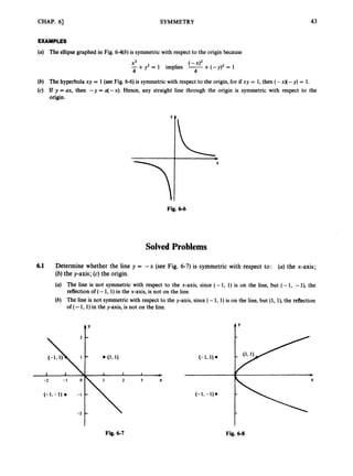
Consider the graph of an equation f ( x , y) = 0. Then, by (i) above, the graph is symmetric with
respect to the y-axis if and only if f ( x , y) = 0 impliesf(-x, y) = 0. And, by (ii) above, the graph is
symmetric with respect to the x-axis if and only iff(x, y) = 0 impliesf(x, -y) = 0.
EXAMPLES
(a) The y-axis is an axis of symmetry of the parabola y = x2 [see Fig. 6-4(u)]. For if y = x2, then y = (- x ) ~ .
The
x-axis is not an axis of symmetry of this parabola. Although (1, 1) is on the parabola, (1, -1) is not on the
parabola.
X L
4
(b) The ellipse -+y2 = 1 [see Fig. 6-4(b)] has both the y-axis and the x-axis as axes of symmetry. For if
X2
-+y2 = 1, then
4
(_x)2+y2= 1 and -+(-y)’=
X2 1
4 4
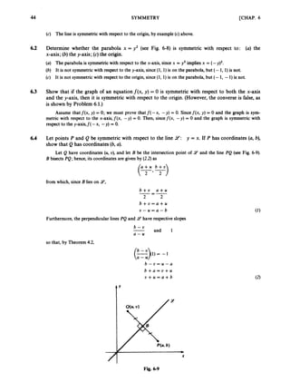
6.2 SYMMETRY ABOUT A POINT
Two points P and Q are said to be symmetric with respect to U point A if A is the midpoint of the
line segment PQ [see Fig. 6-5(u)].
The point Q symmetric to the point P(x,y) with respect to the origin has coordinates (-x, -y). [In
Fig. 6-5(b),APOR is congruent to AQOS. Hence,
Symmetry of a graph about a point is defined in the expected manner. In particular, a graph Y is
said to be symmetric with respect to the origin if, whenever a point P lies on Y, the point Q symmetricto
P with respect to the origin also lies on 9.The graph of an equation f ( x , y) = 0 is symmetric with
respect to the origin if and only iff(x, y) = 0 impliesf( -x, -y) = 0.
= 0sand =a.]
0
t’](https://image.slidesharecdn.com/problemscalculus-221128025033-038ef06f/85/problems-calculus-pdf-55-320.jpg)
![48 FUNCTIONS AND THEIR GRAPHS
1
0
- 1
- 2
-3
[CHAP. 7
0
1
fi 5 1.4
fi z 1.7
2
y = ,
/
=
,
then y2 = 1 - x, and, therefore,x = 1 - y2. Indeed, when x = 1 -y2, then
The range of g therefore consists of all nonnegative real numbers. This is clear from the graph of g [see Fig.
7-5(b)].
The graph is the upper half of the parabola x = 1 -y2.
tY
-1
-’ O I
-3 -2 1 X
(e) A function can be defined “by cases.” For instance,
x2 i f x < o
l + x i f 0 s x s l
Here the valuef(x) is determined by two different formulas.The first formula applies when x is negative, and
the second when 0 5 x s 1. The domain consists of all numbers x such that x 5 1. The range turns out to be
all positive real numbers. This can be seen from Fig. 7-6, in which projection of the graph onto the y-axis
produces all y such that y > 0. .
1 I 1 )
X
Fig. 7-6
Note: In many treatments of the foundations of mathematics, a function is identified with its graph. In
other words, a function is defined to be a setfof ordered pairs such thatfdoes not contain two pairs
(a, b) and (a, c) with b # c. Then “y =j(x))’ is defined to mean the same thing as “(x, y) belongs to 5’’
However, this approach obscures the intuitive idea of a function.
7.2 INTERVALS
convenient to introduce special notation and terminology for them.
In dealing with the domains and ranges of functions, intervals of numbers occur so often that it is](https://image.slidesharecdn.com/problemscalculus-221128025033-038ef06f/85/problems-calculus-pdf-61-320.jpg)
![CHAP. 73 FUNCTIONS AND THEIR GRAPHS 49
Closedintend: [a,b] consists ofall numbers x such that a 5 x 5 b.
The solid dots on the line at a and b means that a and b are included in the closed interval [a, b].
a b
Openintend: (a,b)consists ofall numbers x such that a < x < b.
The open dots on the line at a and b indicate that the endpoints a and b are not included in the open
interval (a,b).
a b
n n
W
Hdf+pen intervals: [a,b)consists ofall numbers x such that a 5 x < b.
a b
(a,b] consists of all numbers x such that a < x s b.
EXAMPLE Consider the functionfsuch thatf(x) = ,
/
=
,
whenever this formula makes sense. The domain off
consists of all numbers x such that
1 - x 2 2 0 or x’11 or - I S X S ~
Thus, the domain off is the closed interval [-1, 13. To determine the range off; notice that as x varies from -1 to
0, x2varies from 1 to 0, 1 - x2 varies from 0 to 1, and ,
/
=
also varies from 0 to 1. Similarly,as x varies from 0
to 1, ,
/
=
varies from 1 to 0. Hence, the range offis the closed interval [0, 13. This is confirmed by looking at
the graph of the equation y = ,
/
=
in Fig. 7-7. This is a semicircle. In fact, the circle x2 +y2 = 1 is equivalent
to
y2 = 1 - x2 or y = +JC7
The value of the functionfcorresponds to the choice of the + sign and gives the upper half of the circle.
- 1
O I
Fig. 7-7](https://image.slidesharecdn.com/problemscalculus-221128025033-038ef06f/85/problems-calculus-pdf-62-320.jpg)
![50 FUNCTIONS AND THEIR GRAPHS [CHAP. 7
Sometimeswe deal with intervalsthat are unbounded on one side.
[a, CO) is made up of all x such that U 5 x.
a
(a, 00) is made up of all x such that a <x.
a
n
V
b
(- CO, b] is made up of all x such that x 5 b.
b
(-CO, b)is made up of all x such that x < b.
n
V
EXAMPLE The range of the function graphed in Fig. 7-6 is (0, CO). The domain of the function graphed in Fig.
7-5(b)is (- CO, 13.
7.3 EVEN AND ODD FUNCTIONS
A functionf is called even if, for any x in the domain off, - x is also in the domain off and
f(-4 =f(x).
EXAMPLES
(a) Letf(x) = x2for all x. Then
f(-x) = (-Xy = x2 =f(x)
and sof is even.
(b) Letf(x) = 3x4 - 5x2 + 2 for all x. Then
f(-x) = 3(-x)4 - 5 ( - X y +2 = 3x4 - 5x2 +2 = f ( x )
Thus,f is even. More generally, a function that is defined for all x and involves only even powers of x is an
even function.
(c) Letf(x) = x3 + 1 for all x. Then
j-(-X) = ( 4 + 1 = 4 + 1
Now -x3 + 1 is not equal to x3+ 1except when x = 0. Hence,fis not even.
A function f is even i
f and only if the graph off is symmetric with respect to the y-axis. For the
symmetry means that for any point (x,f(x)) on the graph, the image point (-x, f (x)) also lies on the
graph; in other words,f(- x) =f ( x )(see Fig. 7-8).](https://image.slidesharecdn.com/problemscalculus-221128025033-038ef06f/85/problems-calculus-pdf-63-320.jpg)
![CHAP. 71 FUNCTIONS AND THEIR GRAPHS 53
EXAMPLE In example (b) above, the polynomial x3 - 5x2 +3x +9 of degree 3 has two roots, -1 and 3,but 3 is
a repeated root of multiplicity 2and, therefore, is counted twice.
Since the complex roots of a polynomial with real coefficients occur in pairs, a f b n , the poly-
nomial can have only an even number (possibly zero) of complex roots. Hence, a polynomial of odd
degree must have at least one real root.
Solved Problems
7.1 Find the domain and the range of the functionfsuch thatf(x) = -x2.
Since -x2 is defined for every real number x, the domain offconsists of all real numbers. To find the
range, notice that x2 2 0 for all x and, therefore, -x2 I
0 for all x. Every non ositive number y appears as
a value -xz for a suitable argument x; namely, for the argument x = &(and also for the argument
x = -A).
Thus the range off is (- 00, 01.This can be seen more easily by looking at the graph of
y = -x2 [see Fig. 7-11(u)].
tY A Y
-I 0 1 X
Fig. 7-11
7.2 Find the domain and the range of the functionfdefined by
The domain off consists of all x such that either -1 < x <0 or 0 Ix < 1. This makes up the open
interval (- 1, 1
)
. The range off is easily found from the graph in Fig. 7-1l
(
b
)
,whose projection onto the
y-axis is the half-open interval [0, 1
)
.
7.3 Definef(x) as the greatest integer less than or equal to x; this value is usually denoted by [x].
Find the domain and the range, and draw the graph off:
Since [x] is defined for all x, the domain is the set of all real numbers. The range offconsists of all
integers. Part of the graph is shown in Fig. 7-12.It consists of a sequence of horizontal, half-open unit
intervals.(A function whose graph consists of horizontal segments is called a stepfunction.)
7.4 Consider the functionfdefined by the formula
x2 - 1
f(x) = -
x - 1
whenever this formula makes sense. Find the domain and the range, and draw the graph off:](https://image.slidesharecdn.com/problemscalculus-221128025033-038ef06f/85/problems-calculus-pdf-66-320.jpg)
![56 FUNCTIONS AND THEIR GRAPHS [CHAP. 7
x2-4x + 5
x3 - 4x2
x - 4 Ix3 - 8x2+ 21x - 20
-4x2 +21x
- 4x2 + 1 6 ~
5x - 20
5x -20
Fig. 7-15
SupplementaryProblems
7.8 Find the domain and the range, and draw the graphs of the functionsdetermined by the followingformulas
(for all arguments x for which the formulasmake sense):
(a) h(x) = 4 - x2 (b) G(x) = -2J;; (c) H(x) = J7.7
J(x)= -Jc7
(f) f ( 4= C2xI
1
(i) F(x) = -
x - 1
3 - x f o r x s l
5x- 3 for x > 1
x i f x s 2
4 i f x > 2
(s) Z(x) = x - [ X I (t) f ( x )= 6
7
.
9 Check your answers to Problem 7.8, parts (a)-(j), (n),@), (
s
)
, (t), by using a graphing calculator.
7.10 In Fig. 7-16, determinewhich sets of points are graphs of functions.
7.11 Find a formula for the function f whose graph consists of all points (x, y) such that (a) x3y - 2 = 0;
(b) x = -
+ ;(c)x2 - 2xy +y2 = 0. In each case, specify the domain off:
1-Y
7.12 For each of the following functions, specify the domain and the range, using interval notation wherever
possible. [Hint: In parts (a),(b), and (e), use a graphing calculator to suggestthe solution.]](https://image.slidesharecdn.com/problemscalculus-221128025033-038ef06f/85/problems-calculus-pdf-69-320.jpg)
![CHAP. 71
-2 - 1 0
FUNCTIONS AND THEIR GRAPHS
w
1 2 X
t Y
I1
X
T'
tY
(4
Fig. 7-16
x2 - 16
i f x # -4
i f x = -4
7.13 (a) Letf(x) = x - 4 and let g(x) = .Determine k so that f ( x ) = g(x) for all x.
X L - x
(b) Let f(4= 7 g(x) = x - 1
Why is it wrong to assert thatfand g are the same function?
7.14 In each of the following cases, define a function having the given set 9 as its domain and the given set 9 as
its range: (a) 9 = (0, 1) and 9 = (0, 2); (b) 9 = [0, 1) and 41 = [- 1
, 4); (c) 9 = [0, 00) and 9 = (0, 1);
(6)9 = (-CO, 1) U (1,2) [that is, (-CO, 1)together with (1,2)] and 41 = (1, CO).
7.15 For each of the functions in Problem 7.8, determine whether the graph of the function is symmetric with
respect to the x-axis, the y-axis, the origin, or none of these.
7.16 For each of the functions in Problem 7.8, determine whether the function is even, odd, or neither even nor
odd.
7.17 (a) Iffis an even function andf(0) is defined, mustf(0) = O?
(b) Iffis an odd function andf(0) is defined, mustf(0) = O?
(c) Iff(x) = x2 +kx + 1for all x and iffis an even function,find k.
(d) Iff(x) = x3 - (k- 2)x2 +2x for all x and iffis an odd function,find k.
(e) Is there a functionfwhich is both even and odd?
7.18 Evaluate the expression f ( x + h,
h
for the following functions$](https://image.slidesharecdn.com/problemscalculus-221128025033-038ef06f/85/problems-calculus-pdf-70-320.jpg)
![58 FUNCTIONS AND THEIR GRAPHS [CHAP. 7
7.19 Find all real roots of the followingpolynomials:
(a) x4 - l0x2 +9 (6) X’ +2x2 - 1 6 ~
- 32 (c) x4 - X’ - l0x2 +4~ +24
(d) x3 - 2x2 +x - 2 (e) x3 +9x2 +26x +24 (f) x3 - 5x - 2 (g) x3 - 4x2 - 2x +8
7.20 How many real roots can the polynomial ax3 +6x2+cx +d have if the coefficients a, 6, c, d are real
numbers and Q # O?
7.21 (a) Iff(x) = (x + 3Xx +k) and the remainder is 16whenf(x) is divided by x - 1,find k.
(6) Iff(x) = (x +5)(x - k) and the remainder is 28 whenf(x) is divided by x - 2, find k.
ALGEBRA The division of a polynomialf(x) by another polynomial g(x)yields the equation
f(x) = s(x)q(x)+ fix)
in which q(x) (the quotient) and r(x) (the remainder) are polynomials, with r(x) either 0 or of lower degree
than g(x). In particular, for g(x) = x - a, we have
f(x) = (x - a)q(x)+ r = (x -aMx) +f(4
that is, the remainder whenf(x) is dioided by x -a isjustf(a).
7.22 If the zeros of a functionf(x) are 3 and -4, what are the zeros of the function g(x) =f(x/3)?
7.23 If f(x) = 2x3+Kx2 +J x - 5, and if f(2) = 3 and f(-2) = -37, which of the following is the value of
K +J?
(i) 0 (ii) 1 (iii) -1 (iv) 2 (v) indeterminate
7.24 Express the set of solutions of each inequality below in terms of the notation for intervals:
(a) 2x + 3 < 9 (6) 5x + 1 2 6 (c) 3x + 4 5 5 (d) 7 ~ - 2 > 8
(e) 3 < 4 x - 5 < 7 (f) - 1 _ < 2 x + 5 < 9 (9) 1 x + 1 ) < 2 (h) 1 3 ~ - 4 1 5 5
(9 yj-
< 1 ( j ) x2 s 6 (k) (X - 3 ) ( ~
+ 1)< 0
2x - 5
7.25 For what values of x are the graphs of (a)f(x) = (x - l)(x +2) and (6)f(x) = x(x - 1)(x+2) above the
x-axis? Check your answers by means of a graphing calculator.
7.26 Prove Theorem 7.1. [Hint: Solvef(r) = 0 for a, ,]
7.27 Prove Theorem 7.2. [Hint: Make use of the ALGEBRA following Problem 721.1](https://image.slidesharecdn.com/problemscalculus-221128025033-038ef06f/85/problems-calculus-pdf-71-320.jpg)
![60 LIMITS [CHAP. 8
PROPERTY 111. If c is a constant andfis a function,
lim c . f ( x ) = c limf(x)
x+a x+a
EXAMPLE
lim 5x = 5 lim x = 5 3 = 15
x 4 3 x+ 3
lim - x = lim (- 1)x = (- 1) lim x = (-1) 3 = -3
X'3 x-3 x-3
PROPERTY IV. Iffand g are functions,
lim [ f ( x ) g(x)] = limf ( x ) lim g(x)
x+a x+a x+a
The limit o
f a product is the product of the limits.
EXAMPLE
lim x2 = lim x lim x = a a = u2
X'O X'O X'O
More generally, for any positive integer n, lim x" = U".
x+o
PROPERTY V. Iffand g are functions,
lim [ f ( x ) g(x)] = limf(x) & lim g(x)
x+a x+a x+a
The limit o
f a sum (diflerence)is the sum (diflerence)of the limits.
EXAMPLES
(4 Iim (3x2+ 5x) = lim 3x2+ lim 5x
x-2 X'2 x-2
= 3 lim x2 + 5 lim x = 3(2)2+ 5(2) = 22
x-2 x-2
(b) More generally, if f ( x ) = a,P +a,- lxn-l + - - - +u0 is any polynomial function and k is any real number,
then
limf(x) = a,k" +u,-lk"-l + +a, = f ( k )
x+k
PROPERTY VI. Iff and g are functions and lim g(x) # 0, then
x+a
x +a
The limit o
f a quotient is the quotient of the limits.
EXAMPLE
lim (2x3- 5)
2(4)3- 5 123
=-=-
2 2 - 5 x+4
lim -
=
x+4 3x +2 lim (3x +2) 3(4) + 2 14
x+4
PROPERTY VII.
lim ,
,
&
j = ,/m
x+a x -+a
The limit o
f a square root is the square root o
f the limit.](https://image.slidesharecdn.com/problemscalculus-221128025033-038ef06f/85/problems-calculus-pdf-73-320.jpg)
![CHAP. 81 LIMITS 61
EXAMPLE
lim ,
/
- = d m= fi = 3
x-42 x+2
Properties IV-VII have a common structure. Each tells us that, providedfand/or g has a limit as x
approaches a (see Section 8.3), another, related function also has a limit as x approaches a, and this
limit is as given by the indicated formula.
83 EXISTENCE OR NONEXISTENCE OF THE LIMIT
In certain cases, a functionf(x) will not approach a limit as x approaches a particular number.
EXAMPLES
(a) Figure 8-l(a)indicates that
1
lim -
x-ro x
does not exist. As x approaches 0,the magnitude of l/x becomes larger and larger. (If x > 0, l/x is positive and
very large when x is close to 0. If x <0, l/xis negative and very “small”when x is close to 0.)
(b) Figure 8-l(b)indicates that
1x1
lim -
x-ro x
does not exist. When x>O, 1x1= x and IxI/x= 1; when x<O, 1x1 = -x and IxI/x= -1. Thus, as x
approaches 0, IxI/x approaches two different values, 1 and -1, depending on whether x nears 0 through
positive or through negative values. Since there is no unique limit as x approaches 0, we say that
1x1
lim -
x-ro x
does not exist.
(4 Let
Then [see Fig. 8-l(c)], limf(x) does not exist. As x approaches 1from the left (that is, through values of x < l
)
,
f ( x )approaches 1.But as x approaches 1 from the right (that is, through values of x > l),f(x) approaches 2
.
x-r 1
(4
Fig. 8-1](https://image.slidesharecdn.com/problemscalculus-221128025033-038ef06f/85/problems-calculus-pdf-74-320.jpg)
![62 LIMITS [CHAP. 8
Notice that the existence or nonexistence of a limit forf ( x ) as x 4a does not depend on the value
f(a), nor is it even required that f be defined at a. If lirnf ( x ) = L, then L is a number to which f ( x ) can
be made arbitrarily close by letting x be sufliciently close to a. The value of L - o r the very existence of
L-is determined by the behavior offnear a, not by its value at a (if such a value even exists).
x+a
Solved Problems
8.1 Find the following limits (if they exist):
(a) Both y2 and l / y have limits as y +2. So, by Property V,
(b) Here it is necessary to proceed indirectly. The function x2 has a limit as x +0. Hence, supposing the
indicated limit to exist, Property V implies that
lim [x' - (x2 - 91= lim -
1
x-0 x+o x
also exists. But that is not the case. [See example (a)in Section 8.3.1 Hence,
lim (x2 -i)
x-0
does not exist.
u2 - 25 (U - 5XU +5)
lim -
-
- lim = lim (U + 5) = 10
"-5 U - 5 "+5 U - 5 U 4 5
(d) As x approaches 2 from the right (that is, with x > 2), [x] remains equal to 2 (see Fig. 7-12). However,
as x approaches 2 from the left (that is, with x < 2), [x] remains equal to 1. Hence, there is no unique
number that is approached by [x] as x approaches 2. Therefore, lirn [x] does not exist.
x + 2
8.2 Find lim f ( x + h, -'@) for each of the following functions. (This limit will be important in the
study of differentialcalculus.)
h - 0 h
1
(a) f ( x )= 3x - 1 (b) f ( x )= 4x2 - x (c) f ( x )=
;
(U) f ( x +h) 3(x +h) - 1 = 3~ +3h - 1
f ( x )= 3x - 1
f ( x +h) - f ( x ) = ( 3 ~
+ 3h - 1) - ( 3 ~
- 1) = 3~ +3h - 1 - 3~ + 1 = 3h
f ( x + h) -fW = - = 3
3h
h h
f ( x +h) - f ( x ) = lim
= 3
h h-0
Hence, lim
h+O](https://image.slidesharecdn.com/problemscalculus-221128025033-038ef06f/85/problems-calculus-pdf-75-320.jpg)
![CHAP. 83 LIMITS 63
(b) f ( x +h) = 4(x +h)’ - (X +h) = 4(x2 +2hx +h2)- x - h
= 4x2 +8hx +4h2 - x - h
f ( x )= 4x2 - x
f(x +h) - f ( x ) = (4x2+8hx +4h2 -x -h) - (4x2- X)
= 4x2 +8hx +4h2 - x - h - 4x2 +x
= 8hx +4h2 - h = h ( 8 ~
+4h - 1)
-
- = 8 ~ + 4 h -1
f(x +h)-f(x) h(8x +4h - 1)
h h
= lim (8x - 1)+lim 4h = 8x - 1 +0 = 8x - 1
h - 0 h+O
1
x + h
(c) f(x +h) = -
1 1
f ( x +h) -f(x) = ---
x + h x
ALGEBRA
a c ad - bc
b d bd
---=-
Hence,
and
x - ( x + ~ ) x - x - ~ -h
--
-
-
-
-
c
(x +h)x (x +h)x (x +h)x
1 1 1 1
.-=--.- = - -
1
= -
lim (x +h) x x x X2
h+O
x3 - 1
8.3 Find lim -
x-1 x - 1 -
Both the numerator and the denominator approach 0 as x approaches 1. However, since 1 is a root of
x3 - 1, x - 1 is a factor of x3 - 1 (Theorem 7.2). Division of x3 - 1 by x - 1 produces the factorization
x3 - 1 = (x - 1Xx2+x + 1).Hence,
x3 - 1 (x - lXX2 +x + 1)
lim -= lim = l i m ( ~ ~ + x + 1 ) = 1 ~ + 1 + 1 = 3
x+l x - 1 x-1 x - 1 X+ 1
[See example (b)following Property V in Section 8.2.1
8.4 (a) Give a precise definition of the limit concept; limf ( x )= L.
x+a
(b) Using the definition in part (a)prove Property V of limits:
limf(x) = L and lirn g(x) = K imply lim [ f ( x )+g(x)] = L +K
x+a x-a x-a](https://image.slidesharecdn.com/problemscalculus-221128025033-038ef06f/85/problems-calculus-pdf-76-320.jpg)
![CHAP. 8) LIMITS 65
SupplementaryProblems
8.5 Find the followinglimits(if they exist):
(a) lim 7
x+2
(4 lim Cxl
~ 4 3 1 2
5u2-4
(b) lim -
u+o U + 1
(e) lim 1x1
x+o
.(h) lim (x - [x])
x-2
4 - w2
(c) lim -
w 4 - 2 w + 2
(f) lim (7x3 - 5x2 +2x -4)
x-*4 x - 4
x 4 2
x2 - x - 12
(i) lim
x3 - x2 - x - 15 2x4 - 7x2 +x -6 x4 +3x3 - 13x2- 2 7 ~
+36
(k) lirn (I) lirn
(n) lim
x - 3 x-2 x - 2 x- 1 x2 +3x - 4
(/I lim
(m) lim
x 4 3
J Z - 2 4
$ x z 3 -fi
x 4 0 X x-1 x - 1 x 4 2
f(x’+ h, and then lirn f ( x -+ h,
h h+O h
(if the latter exists) for each of the following
8.6 Compute
functions:
8.7 Give rigorous proofs of the followingproperties of the limit concept:
(a) lirn x = a (b) lim c = c (c) limf(x) = L for at most one number L
x+a x+a x+a
8.8 Assuming that limf(x) = L and lim g(x) = K,prove rigorously:
x+a x+a
(a) lirn c * f ( x )= c L, where c is any real number,
(b) lim ( f ( x ) g(x)) = L K.
x-a
x+a
x+a
(e) If lim ( f ( x )- L) = 0, then limf(x) = L.
(f) If limf(x) = L = lirn h(x)and iff(x) 5 g(x) 5 h(x) for all x near a, then lim g(x) = L.
x+a x+a
x+a x+a x-a
[Hints:
In part (4,for L > 0,
In part (f),
iff(x) and h(x) lie within the interval (L -E
, L +E), so must g(x).J
8.9 In an epsilon-delta proof of the fact that lirn (2 +5x) = 17, which of the following values of 6 is the
largest that can be used, given E?
x+3](https://image.slidesharecdn.com/problemscalculus-221128025033-038ef06f/85/problems-calculus-pdf-78-320.jpg)
![CHAP. 91 SPECIAL LIMITS 69
to indicate thatf(x) gets larger without bound as x approaches0 from the right [see Fig. 8-l(u)]. Similarly,we
write
1
lim - = -00
x-ro- x
to express the fact thatf(x) decreases without bound as x approaches0 from the left.
- for x > O
(b) Letf ( x )=
[x for x 50
Then (see Fig. 9-3), lim f ( x )= +00 and lim f ( x ) = 0
X’O+ x+O-
t
Fig. 9-3
Whenf(x) has an infinite limit as x approaches a from the right and/or from the left, the graph of
the function gets closer and closer to the vertical line x = a as x approaches U. In such a case, the line
x = a is called a oertical asymptote of the graph. In Fig. 9-4, the lines x = a and x = 6 are vertical
asymptotes(approached on one side only).
If a function is expressed as a quotient, F(x)/G(x),the existence of a vertical asymptote x = U is
usually signaled by the fact that Gfa)= 0 [except when F(a)= 0 also holds].
Fig. 9-4 Fig. 9-5](https://image.slidesharecdn.com/problemscalculus-221128025033-038ef06f/85/problems-calculus-pdf-82-320.jpg)
![70 SPECIAL LIMITS [CHAP. 9
x - 2
x - 3
EXAMPLE Letf(x) = -for x # 3. Then x = 3 is a vertical asymptote of the graph off, because
x - 2 x - 2
3 - +a and lim --
lirn --
x-b3+ x - x+3-
x - 3 - - c o
In this case, the asymptote x = 3 is approached from both the right and the left (seeFig. 9-5).
[Notice that, by division, -- 1
- +- Thus, the graph off@) is obtained by shifting the hyperbola y = l/x
x - 2
x - 3 x - 3 '
three units to the right and one unit up.]
9.3 LIMITS AT INFINITY: HORIZONTAL ASYMPTOTES
As x gets larger without bound, the valuef ( x )of a functionfmay approach a fixed real number c.
In that case, we shall write
lim f ( x )= c
In such a case, the graph off gets closer and closer to the horizontal line y = c as x gets larger and
larger. Then the line y = c is called a horizontal asymptote of the graph-more exactly, a horizontal
asymptote to the right.
X++aD
x - 2
EXAMPLE Consider the functionf(x) = -whose graph is shown in Fig. 9-5. Then lirn f ( x ) = 1 and the line
x - 3 X-.+aD
y = 1is a horizontal asymptote to the right.
Iff(x) approaches a fixed real number c as x gets smaller without bound,' we shall write
lim f ( x ) = c
X ' - W
In such a case, the graph offgets closer and closer to the horizontal line y = c as x gets smaller and
smaller. Then the line y = c is called a horizontal asymptote to the left.
EXAMPLES For the function graphed in Fig. 9-5, the line y = 1 is a horizontal asymptote both to the left and to
the right. For the function graphed in Fig. 9-2, the line y = 0 (the x-axis) is a horizontal asymptote both to the left
and to the right.
If a function f becomes larger without bound as its argument x increases without bound, we shall
write lim f ( x ) = +00.
X + + W
EXAMPLES
lirn (2x + 1)= +oo and lirn x3 = +a
X + + Q ) X - r + a D
If a functionf becomes larger without bound as its argument x decreases without bound, we shall
write lim f ( x ) = +00.
x+--a3
To say that x getssmaller without bound means that x eventuallybecomes smaller than any negative number. Of course, i
n that
case, the absolute value Ix Ibecomes larger without bound.](https://image.slidesharecdn.com/problemscalculus-221128025033-038ef06f/85/problems-calculus-pdf-83-320.jpg)
![CHAP. 93 SPECIAL LIMITS 71
EXAMPLES
lirn x2 = +a and lim --x= +a
.X+-OO x-+-UJ
If a functionfdecreases without bound as its argument x increases without bound, we shall write
lim f ( x )= -CQ.
X++CO
EXAMPLES
lim -2x = -CO and lirn (1 -x2) = --CO
X ' + Q x + + w
If a function f decreases without bound as its argument x decreases without bound, we shall write
lim f ( x )= - W .
x+-CO
EXAMPLES
EXAMPLE Consider the functionfsuch thatf(x) = x - [x] for all x. For each integer n, as x increases from n up
to but not including n + 1,the value off@)increases from 0 up to but not including 1.Thus, the graph consists of a
sequenceof line segments, as shown in Fig. 9-6. Then lirn f ( x ) is undefined, since the valuef(x) neither approaches
a fixed limit nor does it become larger or smaller without bound. Similarly, lim f ( x )is undefined.
x + + m
x-+-OO
-5 -4 -3 -2 -1 1 2 3 4 s x
Fig. 9-6
Finding Limits at Infinity of Rational Functions
3x2 - 5x +2
x + 7
A rational function is a quotient f(x)/g(x)of polynomials f ( x ) and g(x). For example,
x2 - 5
4x' +3x
and are rational functions.
GENERALRULE. Tofind lirn f O a n d lirn -
f ( x ) ,divide the numerator and the denominator by
the highest power of x in the denominator, and then use the fact that
x-++oo g(x) x-'-Q) dx)
C C
lim - = 0 and lim - = 0
x + + m x' x-t-a, x'
for any positive real number r and any constant c.](https://image.slidesharecdn.com/problemscalculus-221128025033-038ef06f/85/problems-calculus-pdf-84-320.jpg)

![Chapter 10
Contlnuity
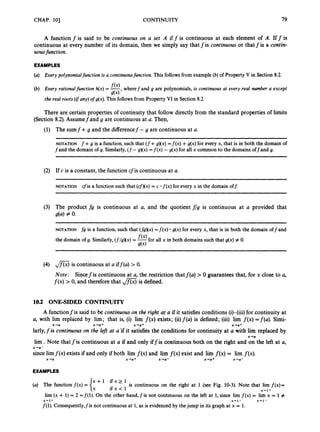
10.1 DEFIMON AND PROPERTIES
can be made precise in the following way.
A function is intuitively thought of as being continuous when its graph has no gaps or juilips. This
D
Definition: A functionfis said t
c
(i) lirn f ( x )exists.
(ii) f(a) is defined.
(iii) lirnf ( x ) =f(a)<
x+a
x-a
EXAMPLES
be continuous at a if the following three conditions hold:
0 i f x = O
1 ifx+O'
The function is discontinuous (that is, not continuous) at 0. Condition (i)is satisfied:
Letf(x) =
lirn f(x) = 1. Condition (ii) is satisfied:f(0) = 0. However, condition (iii) fails: 1 # 0. There is a gap in the
graph off(see Fig. 10-1)at the point (0, 1).The function is continuous at every point different from 0.
Let f(x) = x2 for all x. This function is continuous at every a, since lim f ( ~ )
= lim x2 = a2 =f(a). Notice that
there are no gaps or jumps in the graph off(see Fig. 10-2).
The function f such that f(x) = [x] for all x is discontinuous at each integer, because condition (i) is not
satisfied (see Fig. 7-12). The discontinuities show up asjumps in the graph of the function.
The functionfsuch thatf(x) = Ix I/x for all x # 0 is discontinuous at 0 [see Fig. 8-1(b)]. lirn f(x) does not exist
andf(0) is not defined. Notice that there is a jump in the graph at x = 0.
x-0
x+a x ' U
x-ro
If a functionfis not continuous at a, thenfis said to have a remooable discontinuity at a if a suitable
change in the definition offat Q can make the resulting function continuous at a.
I I
Fig. 10-1 Fig. 10-2
EXAMPLES In example (a)above, the discontinuity at x = 0 is removable, since if we redefinedf so that f(0) = 1,
then the resulting function would be continuous at x = 0. The discontinuities of the functions in examples (c) and
(d)above are not removable.
A discontinuity of a functionfat a is removable if and only if lim f ( x )exists. In that case, the value
x-a
of the function at a can be changed to limf(x).
x+a
78](https://image.slidesharecdn.com/problemscalculus-221128025033-038ef06f/85/problems-calculus-pdf-91-320.jpg)
![80 CONTINUITY [CHAP. 10
(b) The function of example(c) of Section 8.3 [see Fig. 8-l(c)] is continuouson the left,but not on the right at 1.
(c) The function of example(b) of Section 9.1 [see Fig. 9-l(b)] is continuouson the right, but not on the left at 1.
(d) The functionof example (b) of Section 9.2 (seeFig. 9-3) is continuous on the left, but not on the right at 0.
Fig. 10-3
10.3 CONTINUITY OVER A CLOSED INTERVAL
ignoring the function’s behavior at any other points at which it may be defined.
Definition: A functionfis continuous ouer [a, b] if:
(i) fis continuous at each point of the open interval (a,b).
(ii) fis continuous on the right at U.
(iii) fis continuous on the left at b.
We shall often want to restrict our attention to a closed interval [a, b] of the domain of a function,
EXAMPLES
(a) Figure 10-4(a)shows the graph of a functionthat is continuousover [a, b].
2x i f 0 l ; x l ; l
1 otherwise
is continuous over [0, 13 [see Fig. 10-4(b)].
(b) The function f ( x ) =
Note thatfis not continuousat the points x = 0 and x = 1.Observealso that if we redefinedfso thatf(1) = 1,
then the new function would not be continuous over CO, 13, since it would not be continuous on the left at
x = 1.
6 X
(4
Fig. 10-4
ty
A Y
I X](https://image.slidesharecdn.com/problemscalculus-221128025033-038ef06f/85/problems-calculus-pdf-93-320.jpg)
![CHAP. 101 CONTINUITY 81
Solved Problems
x2 - 1
10.1 Find the points at which the functionf(x) = /=if x # -1
is continuous.
For x # -1,fis continuous, sincefis the quotient of two continuous functions with nonzero denomi-
nator. Moreover, for x # -1,
x2 - 1
x + l x + l
(x - 1XX + 1)
f(x) = -
-
- = x - 1
whence lirn f ( x )= lirn (x - 1) = -2 =f( -1).Thus,fis also continuous at x = -1.
x + - 1 x - r - 1
10.2 Consider the function f such that f ( x ) = x - [x] for all x. (See the graph off in Fig. 9-6.) Find
the points at whichf is discontinuous. At those points, determine whether f is continuous on the
right or continuous on the left (or neither).
For each integer n,f(n)= n - [n] = n - n = 0. For n < x < n + l,f(x) = x - [x] = x - n. Hence,
lim f ( x )= lim (x - n) = 0 = f ( n )
x+n+ x+n+
Thus,fis continuous on the right at n.On the other hand,
lim f(x) = lim [x - (n- l)] = n - (n- 1) = 1 # 0 =f(n)
so that f is not continuous on the left at n. It follows thatfis discontinuous at each integer. On each open
interval (n,n + l),fcoincides with the continuous function x - n. Therefore, there are no points of discon-
tinuity other than the integers.
x+n- x-rn-
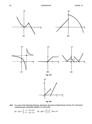
10.3 For each function graphed in Fig. 10-5,find the points of discontinuity (if any). At each point of
discontinuity, determine whether the function is continuous on the right or on the left (or
neither).
(a) There are no points of discontinuity (no breaks in the graph).
(b) 0 is the only point of discontinuity. Continuity on the left holds at 0, since the value at 0 is the number
approached by the values assumed to the left of 0.
(c) 1 is the only point of discontinuity. At 1 the function is continuous neither on the left nor on the right,
since neither the limit on the left nor the limit on the right equalsf(1). (In fact, neither limit exists.)
(d) No points of discontinuity.
(e) 0 and 1 are points of discontinuity. Continuity on the left holds at 0, but neither continuity on the left
nor on the right holds at 1.
f o r O s x s 1
2 x - 2 for k x s 2
.(See Fig. 10-6.)Isfcontinuous over:
10.4 Definef such that f ( x )=
(a) Yes, sincefis continuous on the right at 0 and on the left at 1.
(b) No, sincefis not continuous on the right at 1. In fact,
lim f(x) = lim (2x - 2) = 0 # 1 =f(l)
x + l + % + I +
(c) No, sincefis not continuous at x = 1,which is inside (0,2).](https://image.slidesharecdn.com/problemscalculus-221128025033-038ef06f/85/problems-calculus-pdf-94-320.jpg)
![CHAP. 101 CONTINUITY a3
(a) There are no points of discontinuity [see Fig. 10-7(a)J.At x = O,f(O) = 0 and lim f(x) = 0.
(b) The only discontinuity is at x = 1, since g(1) is not defined [see Fig. 10-7(b)]. This discontinuity is
removable. Since-= (x - ’)(’ -t = x + 1, lim g(x)= lim (x + 1)= 2. So, if we define the func-
tion value at x = 1to be 2, the extended function is continuous at x = 1.
x-0
x2 - 1
x - 1 x - 1 x-. 1 x-. 1
Fig. 10-7
SupplementaryProblems
10.6 Determine the points at which each of the following functions is continuous. (Draw the graphs of the
functions.) Determine whether the discontinuities are removable.
x + l i f x r 2
x - 1 i f x s l
i f l < x < 2
x2 - 4
i f x # -2 i f x z -2
i f x = -2
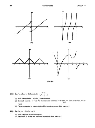
10.7 Find the points of discontinuity (if any) of the functions whose graphs are shown in Fig. 10-8.
10.8 Give simpleexamples of functions such that:
(a) fis defined on [-2,23, continuous over [-1,13, but not continuous over [-2,23.
(b) g is defined on [0, 13,continuous on the open interval (0, l), but not continuous over [0, 1).
(c) h is continuous at all points except x = 0, where it is continuous on the right but not on the left.
10.9 For each discontinuity of the following functions,determine whether it is a removable discontinuity.
(a) The functionfof Problem 7.4 (seeFig. 7-13).
(b) The functionfof example (c) in Section 8.3 [see Fig. 8-l(c)].
(c) The functionfof example (a)in Section 9.1 [see Fig. 9-l(a)].
(d) The functionfin example (a)in Section 9.2 (see Fig. 9-3).
(e) The examples in Problems 10.3and 10.4.](https://image.slidesharecdn.com/problemscalculus-221128025033-038ef06f/85/problems-calculus-pdf-96-320.jpg)
![CHAP. 101 CONTINUITY 85
10.12
10.13
10.14
10.15
10.16
10.17
For each of the followingfunctions determine whether it is continuous over the given interval:
i f x > O
0 ifx=O
(4f(x) = {: over CO, 13
2x i f O < x < l
x - 1 i f x > l
over CO, 11 (d) f as in part (c) over Cl, 21
X’ - 16
i f x # 4
If the functionf(x) = [
T is continuous, what is the value of c?
cc i f x = 4
x2 - b2
Let b # 0 and let g be the function such that g(x) = 1- i f x # b
lo ifx = b
(a) Does g(b)exist? (b) Does lim g(x) exist? (c) Is g continuous at b?
x-+b
(a) Show that the followingf is continuous:
c7b i f x = 6
(b) For what value of k is the followinga continuous function?
U i f x = 2
Determine the points of discontinuity of the following functionf:
1 if x is rational
0 if x is irrational
[Hint: A rational number is an ordinary fraction p/q, where p and q are integers. Recall Euclid’s proof that
fi cannot be expressed in this form; it is an irrational number, as must be &I, for any integer n. It
follows that any fixed rational number r can be approached arbitrarily closely through irrational numbers
of the form r +&/n. Conversely, any fixed irrational number can be approached arbitrarily closely
through rational numbers.]
U
s
e a graphing calculator to find the discontinuities (if any) of the followingfunctions](https://image.slidesharecdn.com/problemscalculus-221128025033-038ef06f/85/problems-calculus-pdf-98-320.jpg)
![Chapter 11
The Slope of a Tangent Line
The slope of a tangent line to a curve is familiar in the case of circles [see Fig. 11-l(u)]. At each
point P of a circle, there is a line 9 such that the circle touches the line at P and lies on one side of the
line (entirely on one side in the case of a circle). For the curve of Fig. 11-l(b), shown in dashed lines, Y 1
is the tangent line at P,, 9, the tangent line at P,, and 9,
the tangent line at P,. Let us develop a
definition that corresponds to these intuitive ideas about tangent lines.
Figure ll-2(u) shows the graph (in dashed lines) of a continuous functionf: Remember that the
graph consists of all points (x, y ) such that y =f(x). Let P be a point of the graph having abscissa x.
Then the coordinates of P are (x,~(x)).
Take a point Q on the graph having abscissa x +h. Q will be
close to P if and only if h is close to 0 (becausefis a continuous function). Since the x-coordinate of Q is
x +h, the y-coordinate of Q must bef(x +h). By the definition of slope, the line PQ will have slope
f ( x +h) -fW -
- f ( x +h) -m
(X +h) -x h
Observe in Fig. ll-2(6)what happens to the line PQ as Q moves along the graph toward P. Some of
the positions of Q have been designated as Q1,
Q2,Q 3 , ..., and the corresponding lines as A,,A2,
Fig. 11-1
4 y
I I b b
X x + h X X
( a) ( 6 )
Fig. 11-2
86](https://image.slidesharecdn.com/problemscalculus-221128025033-038ef06f/85/problems-calculus-pdf-99-320.jpg)
 = (xz +2xh +hZXx+h)
= (x3+2x2h +h2x)+(x2h+2xh2 +h3)
= x3 +3x2h +3xhZ+h3
Hence,
and
f ( x +h) -f(x) = (x3+3x2h +3xh2 +h3)- x3
= 3x2h +3xh2 +h3 = h(3x2+ 3xh +h2)
f ( x +h) -f(x) h(3x2 +3xh +h2)
= 3x2 + 3xh +h2
-
-
h h
lim f ( x + h, - f ( x ) = lim (3x2+ 3xh +h2)
h - 0 h h-0
= 3x2 +3 ~ ( 0 )
+O2 = 3x2
This shows that the slope of the tangent line at P is 3x2. For example, the slope of the tangent line at (2, 8)
is 3x2 = 3(2)2= 3(4)= 12.
11.3 (a) Find a formula for the slope of the tangent line at any point of the graph of the functionf
such thatf ( x )= l/x(the hyperbola in Fig. 11-5).
(b) Find the slope-interceptequation of the tangent line to the graph offat the point (2, i).
1 1
f ( x +h) = - and f ( x ) =
;
x + h
h
= --
1 1 x - ( x + ~ )
- x - x - ~
f ( x +h) -f(x) = -- -= -
x +h x (x +h)x (x +h)x (x +h)x
'f:
I
Fig. 11-5](https://image.slidesharecdn.com/problemscalculus-221128025033-038ef06f/85/problems-calculus-pdf-101-320.jpg)
![90 THE SLOPE OF A TANGENT LINE [CHAP. 11
(b) From part (a), the slope of the tangent line at (0, 4) is 6x - 6 = 6
(
0
)- 6 = 0 - 6 = -6. Hence, the
slope-intercept equation has the form y = -6x +6. Since the line passes through (0,4), the y-intercept
b is 4. Thus, the equation is y = -6x +4.
(c) We want the graph of y = 3x2 - 6x +4. Complete the square:
y = 3 x 2 - 2 x + - = 3 ( x - l ) 2 + - =3(x-1)2+1
( 3 ( :>
The graph (see Fig. 11-6)is obtained by moving the graph of y = 3x2 one unit to the right [obtaining
the graph of y = 3(x - l)'] and then raising that graph one unit upward.
-
I 2 x
"1 Fig. 11-6
11.5 The normal line to a curve at a point P is defined to be the line through P perpendicular to the
tangent line at P. Find the slope-intercept equation of the normal line to the parabola y = x2 at
the point (4,
a). I
By Problem 11.1, the tangent line has slope 2(f) = 1. Therefore, by Theorem 4.2, the slope of the
normal line is - I, and the slope-intercept equation of the normal line will have the form y = - x +b.
When x = f,y = x2 = (4)' = 4, whence,
3
4 4
-
' = - ( ' ) + b or b = -
Thus, the equation is
3
y = - x + -
4
Supplementary Problems
11.6 For each function f and argument x = a below, (i) find a formula for the slope of the tangent line at an
arbitrary point P(x,f ( x ) )of the graph off; (ii) find the slope-intercept equation of the tangent line corre-
sponding to the given argument a; (iii)draw the graph offand show the tangent line found in (ii).
(a) f ( x )= 2x2 +x; a = - (b) f ( x )= - x3 + 1; a = 2
1
(c) f ( x ) = x2 - 2x; a = 1 (d) f ( x )= 4x2 +3; a = -
2
1 1
4 3](https://image.slidesharecdn.com/problemscalculus-221128025033-038ef06f/85/problems-calculus-pdf-103-320.jpg)
![CHAP. 113 THE SLOPE OF A TANGENT LINE 91
11.7 Find the point(s) on the graph of y = x2 at which the tangent line is parallel to the line y = 6x - 1. [Hint:
Use Theorem 4.1.)
11.8 Find the point(s) on the graph of y = x3 at which the tangent line is perpendicular to the line 3x +9y = 4.
[Hint: Use Theorem 4.2.1
11.9 Find the slope-interceptequation of the line normal to the graph of y = x3at the point at which x = 4.
11.10 At what point(s)does the line normal to the curve y = x2 - 3x +5 at the point (3, 5) intersect the curve?
11.11 At any point (x, y) of the straight line having the slope-intercept equation y = mx +b, show that the
tangent line is the straight line itself.
11.12 Find the point(s) on the graph of y = x2 at which the tangent line is a line passing through the point
(2, -12). [Hint: Find an equation of the tangent line at any point (xo, xi) and determine the value@)of xo
for which the line contains the point (2, -12).]
11.13 Find the slope-intercept equation of the tangent line to the graph of y = fi at the point (4, 2). [Hint: See
ALGEBRA in Problem 10.15.1](https://image.slidesharecdn.com/problemscalculus-221128025033-038ef06f/85/problems-calculus-pdf-104-320.jpg)
![Chapter 12
The Derivative
The expression for the slope of the tangent line
f ( x +h) -f(4
h
lirn
h-+O
determines a number which depends on x. Thus, the expression defines a function, called the derivative
Definition: The derivativef’ offis the function defined.by the formula
off.
NOTATION There are other notations traditionallyused for the derivative:
dY
D,f(x) and -
dx
dY
When a variable y representsf(x), the derivative is denoted by y’, D,y, or - We shall use whichever notation is
dx *
most convenient or customary in a given case.
The derivative is so important in all parts of pure and applied mathematics that we must devote a
great deal of effort to finding formulas for the derivatives of various kinds of functions. If the limit in the
above definition exists, the functionfis said to be dz@erentiabZe at x, and the process of calculatingf‘ is
called diferentiation off.
EXAMPLES
(a) Letf(x) = 3x +5 for all x. Then,
Hence,
f(x +h) = 3(x +h) +5 = 3x +3h +5
f(x +h) -f(x) = ( 3 ~
+ 3h +5) - ( 3 ~
+ 5) = 3x + 3h + 5 - 3x - 5 = 3h
S(X + h) -I@)-
- - = 3
3h
h h
f(x + h) -f(x) = lim =
h h+O
f’(x)= lim
h+O
or, in another notation, D,(3x +5) = 3. In this case, the derivativeis independent of x.
(b) Let us generalizeto the case of the functionf(x) = Ax +B, where A and B are constants.Then,
f(x +h) - f ( x ) [A(x +h) +B] - (Ax +B) AX +Ah +B - AX - B Ah
-
- -
- = - - = A
h h h h
Thus, we have proved:
Theorem12.1: D,(Ax +B) = A
By letting A = 0 in Theorem 12.1, we obtain:
92](https://image.slidesharecdn.com/problemscalculus-221128025033-038ef06f/85/problems-calculus-pdf-105-320.jpg)
![T
EXAMPLES
THE DERIVATIVE [CHAP. 12
D,(x4) = 44x3 x)
ALGEBRA
= x3 D,(x) +x D,(x3) [by the product rule]
= x3(1) +x(3x2) = x3 +3x3 = 4x3
D,(xS) = D,(x4 x)
= x4 D,(x) +x D,(x4)
= x4(1) +x(4x3)
= x4 +4x4 = 5x4
[by the product rule]
[by example (a)]
DX((x3+x)(x2- x +2)) = (x3 +X) D,(x' - x +2) +(x' - x +2) D,(x3 +X)
= (x3+x)(~x
- 1) +(x2 - x +2 x 3 ~ '+ 1)
The reader may have noticed a pattern in the derivativesof the powers of x:
D,(x) = 1 = 1 xo D,(x2) = 2x D,(x3) = 3x2 Dx(x4)= 4x3 Dx(x5)= 5x4
This pattern does in fact hold for all powers of x.
RULE 4. D,(x") = nx"-'
where n is any positive integer.
For a proof, see Problem 12.2.
EXAMPLES
(U) D,(x9) = 9x8
(b) D,(~x") = 5 D,(x") = 5(11x1O)= 55x"
Using Rules 1,2, and 4, we have an easy method for differentiatingany polynomial.
EXAMPLE
Dx(; x3- 4x2 +2x - ;
) = D X ( i 2)- DX(4X2)+Dx(2x)- D,(i) [by Rule 1
3
3
5
3
5
= - D,(x3) -4 D,(x2) +2 D,(x) - 0 [by Rule 2 and Corollary 12.2)
[by Rule 41
= - (3x7 - 4 (24 +2 (1)
9
5
-
- - x2 - 8~ +2
More concisely,we have:
RULE 5. To differentiatea polynomial,change each nonconstant term akxk to kakxk-' and drop the
constant term (if any).
EXAMPLES
(a) D,(8x5 - 2x4 +3x2+5x +7) = 40x4-8x3 +6x +5
8
3
4
3
3x7 +8 x 5 -- x2 +9x - It = 21x6 + 5 8 x 4 -- x +9](https://image.slidesharecdn.com/problemscalculus-221128025033-038ef06f/85/problems-calculus-pdf-107-320.jpg)
![CHAP. 121 THE DERIVATIVE 95
SolvedProblems
12.1 Prove: (a)Rule l(i, ii);(b) Rule 2. Assume that D,f(x) and Ox&) are defined.
cCf(x + h) -fWI
h
= lim
c *f(x+h) - c *f(x)
h h+O
(b) D,(c *f(x))= lim
h+O
f ( x + h, -
'
(
'
)
h
[by Section 8.2, Property 1111
= c lim
h-rO
= c D,f(x)
12.2 Prove Rule 4, D,(x") = nx"- ',for any positive integer n.
We already know that Rule 4 holds when n = 1,
D,(X') = D,(x) = 1 = 1 xo
(Remember that xo = 1.)We can prove the rule by mathematical induction. This involves showing that if
the rule holdsfor any particular positive integer k, then the rule also must holdfor the next integer k + 1. Since
we know that the rule holds for n = 1,it would then follow that it holds for all positive integers.
Assume, then, that D&ck) = kx'-'. We have
D,(xk+ = Dx(xk x) [since xk+1= x k x1 = xk x]
= Xk D,(x) +x D,(xk)
= xk 1 +x(kx"-')
= xk +kx'
= (1 + k)xk= (k + l)x(k+l)-l
[by the product rule]
[by the assumption that Dx(x")= kxk-']
[since x 2 - 1 = x1 2 - 1 = xkl
and the proof by induction is complete.
12.3 Find the derivative of the polynomial 5x9 - 12x6+4x5 - 3x2 +x - 2.
By Rule 5,
D,(5x9 - 12x6+4x5 - 3x2 +x -2) = 4 5 ~ '
- 72x5+20x4 - 6x + 1
124 Find the slope-interceptequations of the tangent lines to the graphs of the followingfunctions at
the given points:
(a) f ( x )= 3x2 - 5x + 1, at x = 2
(a) Forf(x) = 3x2 - 5x + 1,Rule 5 givesf'(x) = 6x - 5. Then,
(b) f ( x )= x7 - 12x4+2x, at x = 1
f'(2) = 6(2)-5 = 12 - 5 = 7
f(2) = 3(2)2- 5(2)+ 1
and 3(4) - 10 + 1 = 12 - 9 = 3
Thus, the slope of the tangent line to the graph at (2, f(2)) = (2, 3) is f'(2) = 7, and we have as a
point-slope equation of the tangent line y - 3 = 7(x -2), from which we get
JJ- 3 = 7~ - 14
y = 7 x - 11](https://image.slidesharecdn.com/problemscalculus-221128025033-038ef06f/85/problems-calculus-pdf-108-320.jpg)
![Chapter 13
More on the Derivative
13.1 DIFFERENTIABILITY AND CONTINUITY
In the formula lim + h,
h-0 h
for the derivativef’(a), we can let x = a +h and rewritef’(a) as
lim j
(
’
) Iffis differentiable at a, then
x-0
limf ( x )= lim [ f ( x )-f(a) +f(a)]
x+a x+a
= lim [ f ( x )-f(a)] +limf(a)
x+a x+a
=f’(a) 0 +f(a) =f(a)
Thus,fis continuous at a. This proves:
Tkorem 13.1: Iffis differentiable at a, thenfis continuous at a.
EXAMPLE Differentiability is a stronger condition than continuity. In other words, the converse of Theorem 13.1
is not true. To see this, consider the absolute-value functionf(x) = 1x1 (see Fig. 13-1).fis obviously continuous at
x = 0; but it is not differentiableat x = 0. In fact,
h - 0
= lim -- - l i m 1 = 1
f(0+ h) -f(O)
h h-+O+ h-O+
lirn
h+O+
- h - 0
lim f(O + h, -f(o) = lim -
= lim - 1 = -1
h-0- h h-+O- h - 0 -
and so the two-sided limit needed to definef’(0) does not exist. (The sharp corner in the graph is a tip-off. Where
there is no unique tangent line, there can be no derivative.)
X
Fig. 13-1
99](https://image.slidesharecdn.com/problemscalculus-221128025033-038ef06f/85/problems-calculus-pdf-112-320.jpg)
![CHAP. 131 MORE ON THE DERIVATIVE 101
1
3
.
2 Prove Rule 6, the quotient rule: Iffand g are differentiable at x and if g(x) # 0, then
If g(x) # 0, then l/g(x) is defined. Moreover, since g is continuous at x (by Theorem 13.1), g(x +h) # 0
for all sufficientlysmall values of h. Hence, l/g(x +h) is defined for those same values of h. We may then
calculate
1 1
g(x) -g(x +
- h, [by algebra: multiply top and bottom by g(x)g(x +h)]
9(x +h) g(x)= lim
h h-0 hg(xk(x + h
,
lim
h-rO
lim c-l/S(X)l
lim g(x +h) D,g(x) [by Property VI of limits and differentiability of g]
h+O
-
-
h-rO
[by Property I1 of limits and continuity of g]
-l/gW .Dxg(x)
=-
g(x)
-1
=-
[g(x)I2 Dx g(x)
Having thus proved that
we may substitute in the product rule (proved in Problem 13.1) to obtain
which is the desired quotient rule.
13.3 Prove Rule 7:Dx(xk)= kxL-' for any integer k.
When k is positive, this is just Rule 4 (Chapter 12).When k = 0,
DJxk) = Dx(xo)= Dx(l)= 0 = 0 x-' = kxk-'
Now assume k is negative; k = -n, where n is positive.
~ ~~
ALGEBRA By definition,
By (1)of Problem 13.2,
-1](https://image.slidesharecdn.com/problemscalculus-221128025033-038ef06f/85/problems-calculus-pdf-114-320.jpg)
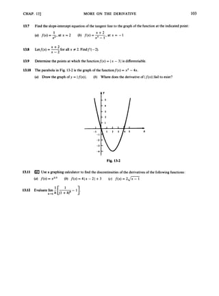
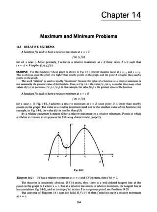
![CHAP. 14) MAXIMUM AND MINIMUM PROBLEMS 105
A Y
2 -
1 -
I *
I 2 X
Fig. 14-2 Fig. 14-3
EXAMPLE Consider the functionf(x) = x3. Becausef’(x) = 3x2,f’(x) = 0 if and only if x = 0. But from the graph
offin Fig. 14-3it is clear thatfhas neither a relative maximum nor a relative minimum at x = 0.
In Chapter 23, a method will be given that often will enable us to determine whether a relative
extremum actually exists whenf’(c) = 0.
14.2 ABSOLUTE EXTREMA
Practical applications usually call for finding the absolute maximum or absolute minimum of a
function on a given set. Letfbe a function defined on a set d (and possibly at other points, too), and let
c belong to b. Then f is said to achieve an absolute maximum on Q at c if f ( x )<f(c) for all x in b.
Similarly,fis said to achieve an absolute minimum on E at d iff(x) >f(d) for all x in 8.
If the set d is a closed interval [a, b], and if the functionfis continuous over [a, b] (see Section
1
0
.
3
)
,
then we have a very important existence theorem (which cannot be proved in an elementary way).
Theorem14.2 (Extreme-Value Theorem): Any continuous function f over a closed interval [a, b] has
an absolute maximum and an absolute minimum on [a, b].
EXAMPLES
(a) Letf(x) = x + 1 for all x in the closed interval [0, 21. The graph offis shown in Fig. 14-*a). Thenfachieves
an absolute maximum on CO, 2) at x = 2; this absolute maximum value is 3. In additionJachieves an absolute
minimum at x = 0; this absolute minimum value is 1.
(b) Let f(x) = l/x for all x in the open interval (0, 1). The graph off is shown in Fig. 14-4(b).f has neither an
absolute maximum nor an absolute minimum on (0, 1). If we extendedf to the half-open interval (0, 11, then
there is an absolute minimum at x = 1,but still no absolute maximum.
x + l i f - l < x < O
ifx=O
Iox - 1 i f O < x < l
(4 k t f ( x ) =
See Fig. 14-q~)
for the graph off: f has neither an absolute maximum nor an absolute minimum on the
closed interval [- 1, 13.Theorem 14.2does not apply, becausefis discontinuous at 0.
Critical Numbers
To actually locate the absolute extrema guaranteed by Theorem 14.2,it is useful to have the follow-
ing notion.](https://image.slidesharecdn.com/problemscalculus-221128025033-038ef06f/85/problems-calculus-pdf-118-320.jpg)
![106 MAXIMUM AND MINIMUM PROBLEMS [CHAP. 14
(6)
Fig. 14-4
Definition: A critical number of a functionfis a number c in the domain off for which eitherf’(c) = 0
orf’(c) is not defined.
EXAMPLES
(a) Let f ( x ) = 3x2-2x +4. Then f‘(x) = 6x - 2. Since 6x - 2 is defined for all x, the only critical numbers are
given by
6 ~ - 2 = 0
6x = 2
X = $ = i
Thus, the only critical number is 3.
(b) Letf(x) = x3 -x2 -5x +3. Thenf’(x) = 3x2 -2x -5, and since 3x2 - 2x -5 is defined for all x, the only
critical numbers are the solutions of
3x2 -2x - 5 = 0
(3x - 5)(x + 1) = 0
3 x - 5 = 0 or x + 1 = 0
3x = 5 or x = - 1
x = 3 or x - -1
Hence, there are two critical numbers, -1 and 3.
We already know from the example in Section 13,l thatf’(0)is not defined. Hence, 0 is a critical number.
SinceD,(x) = 1and DA-x) = -1, there are no other critical numbers.
Method for FindingAbsolute Extrema
Let f be a continuous function on a closed interval [a, b]. Assume that there are only a finite
number of critical numbers c1, c2, ...,ck off inside [a, b]; that is, in (a, b). (This assumption holds for
most functions encountered in calculus.) Tabulate the values off at these critical numbers and at the
endpoints U and b, as in Table 14-1. Then the largest tabulated value is the absolute maximum off on
[a, b], and the smallest tabulated value is the absolute minimum off on [a, b].(This result is proved in
Problem 14.1.)](https://image.slidesharecdn.com/problemscalculus-221128025033-038ef06f/85/problems-calculus-pdf-119-320.jpg)

![108 MAXIMUM AND MINIMUM PROBLEMS [CHAP. 14
2/3
1
-1
2
By the extreme-value theorem (Theorem 14.2), a functionfcontinuous on [a, b] must have an absolute
maximum and an absolute minimum on [a, b]. Let p be an argument at which the absolute maximum is
achieved.
CaseZ: p is one of the endpoints, a or b. Thenf(p) will be one of the values in our table. In fact, it will be
the largest value in the table, sincef(p) is the absolute maximum offon [a, b].
Case 2: p is not an endpoint andf’(p) is not defined. Then p is a critical number and will be one of the
numbers c1, c2, ...,ck in our list. Hence,f(p) will appear as a tabulated value, and it will be the largest of
the tabulated values.
Case 3.- p is not an endpoint and f‘b)
is defined. Since p is the absolute maximum off on [a, b],
f(p) 2f(x) for all x near p. Thus,fhas a relative maximum at p, and Theorem 14.1 givesf’b) = 0. But then
p is a critical number, and the conclusion follows as in Case 2.
A completely analogous argument shows that the method yields the absolute minimum.
1/27
0
-12 min
3 max
14.2 Find the absolute maximum and minimum of each function on the given interval:
x2 +3
(a) f ( x )= 2x3 - 5x2 +4x - 1 on [-I, 2) (6) f ( x ) = x+l on CO,31
(a) Sincef’(x) = 6x2 - 10x +4, the critical numbers are the solutions of:
6x2 - 10x +4 = 0
3x2 - 5x +2 = 0
( 3 ~
- 2)(x - 1)= 0
3 x - 2 = 0 or x - 1 = 0
3x = 2 or x = l
x = 3 or x = l
Thus, the critical numbers are 3 and 1, both of which are in (- 1,2). Now construct Table 14-3:
f
(
’
) = 2
(
‘
)
3 - ( ‘ ) l + 4
(
;
) - = -
16 - -
20+8
- - = -
16 - -
60 + -
72 - -
27 = -
1
27 9 3 27 27 27 27 27
f(i) = 2(1)3 - 5(i)2 +qi)- 1 = 2 - 5 +4 - 1 = o
f(- 1) = 2(- 1)3- 5(- 1)2+4(- 1) - 1 = -2 - 5 - 4 - 1 = - 12
f(2) = 2(2)3- 5(2)2+q2) - 1 = 16 - 20 +8 - 1 = 3
Thus, the absolute maximum is 3, achieved at x = 2, and the absolute minimum is - 12, achieved at
x = -1.
Table 14-3
(X + l)DX(x2+3) - (x’ +3)DX(x+ 1) - (X + 1x2~)
- (x’ +3x1)
2x2 +2x - x2 - 3
(x + 1)2
-
(x + 1)2 (x + 1)2
(4 f ’ ( 4 =
x2 +2x - 3
(x + 1)2
-
-
-
-
f’(x) is not defined when (x + 1)2= 0; that is, when x = -1. But since - 1 is not in (0, 3), the only
critical numbers that need to be considered are the zeros of x2 +2x - 3 in (0, 3):
x2 + 2x - 3 = 0
(X+ 3 ) ( ~
- 1) = 0
x + 3 = 0 or x - 1 = 0
x = -3 or x = l](https://image.slidesharecdn.com/problemscalculus-221128025033-038ef06f/85/problems-calculus-pdf-121-320.jpg)
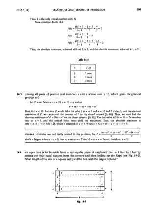
![110 MAXIMUM AND MINIMUM PROBLEMS [CHAP. 14
Let x be the side of the square that is removed from each corner. The volume V = Iwh, where I, w, and
h are the length, width, and height of the box.Now 1 = 8 - 2x, w = 3 - 2x, and h = x, giving
V(X)= (8 - 2xK3 -2x)x = (4x2 - 2 2 ~
+2 4 ) ~
= 4 2 - 22x2 +2 4 ~
The width w must be positive. Hence,
3 - 2 x > O or 3 > 2 x or 3 > x
Furthermore, x > 0. But we also can admit the values x = 0 and x = 3, which make V = 0 and which,
therefore, cannot yield the maximum volume. Thus, we have to maximize V(x)on the interval CO, 31.Since
-=
dV 12x2 -4 4 ~
+24
dx
the critical numbers are the solutions of
12x2- 4 4 ~
+24 = 0
3x2 - llx +6 = 0
(3x - 2xx - 3) = 0
3 x - 2 = 0 or x - 3 = 0
3x = 2 or x = 3
x = j or x = 3
The only critical number in (0,j)is 3. Hence, the volume is greatest when x = 3.
14.5 A manufacturer sells each of his TV sets for $85. The cost C (in dollars) of manufacturing and
sellingx TV sets per week is
C = 1500 + 10x +0 . 0 0 5 ~ ~
If at most loo00 sets can be produced per week, how many sets should be made and sold to
maximizethe weekly profit?
For x sets per week, the total income is 85x. The profit is the income minus the cost,
P = 8 5 ~
- (1500+ 1 0 ~
+0 . 0 0 5 ~ ~ )
= 7 5 ~
- 1500 -0 . 0 0 5 ~ ~
We wish to maximize P on the interval CO, lOOOO], since the output is at most 1OOOO.
--
- 75 -0.01x
dP
dx
and the critical number is the solution of
75 - 0.01x = 0
0.01x= 75
x=-- 75 - 7500
0.01
We now construct Table 14-5:
P(7500) = 75(7500) - 1500 - 0.0005(7500)2
= 562500 - 1500-0.0005(56250000)
= 5
6
1OOO - 281250 = 279750
P(0)= 75(0) - 1500-0.0005(0)2= -1500
P(1OOOO)= 75(10000) - 1500 - 0.0005(10000)2
750OOO - 1500 -O.OOOS( 100OOOOOO)
= 748 500 - 500000 = 248 500
Thus, the maximum profit is achieved when 7500 TV sets are produced and sold per week.](https://image.slidesharecdn.com/problemscalculus-221128025033-038ef06f/85/problems-calculus-pdf-123-320.jpg)
![CHAP. 141 MAXIMUM AND MINIMUM PROBLEMS 111
Table 14-5
279750
248 500
-1500
14.6 An orchard has an average yield of 25 bushels per tree when there are at most 40 trees per acre.
When there are more than 40 trees per acre, the average yield decreases by 9 bushel per tree for
every tree over 40. Find the number of trees per acre that will give the greatest yield per acre.
Let x be the number of trees per acre, and let f(x) be the total yield in bushels per acre. When
0 sx 5 40,f(x) = 25x. If x > 40, the number of bushels produced by each tree becomes 25 - i(x - 40).
[Here x -40 is the number of trees over 40, and i(x -40) is the corresponding decrease in bushels per
tree.] Hence, for x > 40,f(x) is given by
1 X
(X -40)). = (25 --
2 x +2 0 ) ~= (45 - f X)X = (90 - X)
Thus,
X
f ( x ) is continuous everywhere, since 25x =-(90 - x) when x = 40. Clearly,f(x) < 0 when x > 90.Hence,
we may restrict attention to the interval CO,901.
For 0 < x < 40,f ( x )= 25x, and f’(x)= 25. Thus, there are no critical numbers in the open interval
(0,40). For 40 < x < 90,
2
X X2
f(x) = -.(90 -X) = 4 5 ~
--
2 2
and f’(x)= 45 - x
Thus, x = 45 is a critical number. In addition, 40 is also a critical number sincef‘(40) happens not to exist.
We do not have to verify this fact, since there is no harm in adding 40 [or any other number in (0, 9O)J to
the list for which we computef(x).
We now construct Table 14-6:
f(45) = -
45 (90 -45) = -
45 (45) = -
2025 = 1012.5
2 2 2
f(40) = 25(40) = loo0
f(0)= 25(0) = 0
90 90
f(90) = -(90 -90) = -(0) = 0
2 2
The maximum yield per acre is realized when there are 45 trees per acre.
Table 14-6](https://image.slidesharecdn.com/problemscalculus-221128025033-038ef06f/85/problems-calculus-pdf-124-320.jpg)
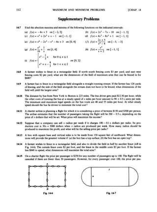
![114 MAXIMUM AND MINIMUM PROBLEMS [CHAP. 14
14.22 Find the height h and the radius r of the right circular cylinder of greatest volume that can be inscribed in a
sphere of radius U. [Hint: See Fig. 14-9. The Pythagorean theorem relates h/2 and r, and provides bounds
on each.]
14.23 Among all isosceles triangles with a fixed perimeter p, which has the largest area? [Hint: See Fig. 14-10 and
solve the equivalent problem of maximizing the square of the area.]
x2 y2
14.24 Find the point(s) on the ellipse -+-= 1 that is (are): (a)closest to the point (1,O);(6)farthest from the
25 9
point (1, 0
)
.[Hint: It is easier to find the extrema of the square of the distance from (1, 0) to (x, y). Notice
that - 5 I
x I
5 for points (x, y) on the ellipse.]
14.25 A rectangular swimming pool is to be built with 6-foot borders at the north and south ends, and 10-foot
borders at the east and west ends. If the total area available is 6OOO square feet, what are the dimensions of
the largest possible water area?
14.26 A farmer has to enclose two fields. One is to be a rectangle with the length twice the width, and the other is
to be a square. The rectangle is required to contain at least 882 square meters, and the square has to
contain at least 400 square meters. There are 680 meters of fencing available.
(a) If x is the width of the rectangular field, what are the maximum and minimum possible values of x?
(b) What is the maximum possible total area?
14.27 It costs a company 0 . 1 ~ ~
+4x +3 dollars to produce x tons of gold. If more than 10 tons is produced, the
need for additional labor raises the cost by 2(x - 10)dollars. If the price per ton is $9, regardless of the
production level,and if the maximum production capacity is 20 tons, what output maximizes the profit?
f(c+ h, -f(c) 0 for h
h
14.28 Prove Theorem 14.1. [Hint: Take the case of a relative minimum at x = c. Then
f(c + h,
h
sufficiently small and positive, and
Sincef’(c) exists,f’(c) = lirn f(c + h, -
’
(
‘
) 2 0 andf’(c) = lim
I
0 for h negative and sufficiently small in magnitude.
f(c + h) --f(c) ~ 0*1
h
h+O+ h h - 0 -
14.29 A rectangle is inscribed in an isosceles triangle with base 9 inches and height 6 inches. Find the dimensions
of the rectangle of maximum area if one side of the rectangle lies inside the base of the triangle.
14.30 A rectangular yard is to enclose an area of 200 square meters. Fencing is required on only three sides, since
one side will lie along the wall of a building. The length and width of the yard are each required to measure
at least 5 meters.
(a) What dimensions will minimize the total fencing required? What will be the minimum fencing?
(b) What dimensions will maximize the total fencing, and what will be the maximum fencing?
2x - 3
14.31 Letf(x) = -
x2 *
(a) Find the maximum and minimum values offon [l, 101.
(b) Does the extreme-value theorem apply tofon [-10, lO]? Why?
14.32 Find the point@)on the curve y = ,/6x4 +8x3 + 1lx2+9 that is (are) closest to the origin.
14.33 Find the shortest distance between points of the curve y = ,/x2 + 3x +2 and the origin.
14.34 Find the dimensions of the rectangle of maximum area that can be inscribed in a right triangle whose sides
are 3, 4, and 5, if one side of the rectangle lies on the side of the triangle of length 3 and the other side lies
on the side of the triangle of length 4.](https://image.slidesharecdn.com/problemscalculus-221128025033-038ef06f/85/problems-calculus-pdf-127-320.jpg)
![CHAP. 151 THE CHAIN RULE 117
(6) Letf(x) = x2 +2x and g(x) = &.Then,
Again,g 0 fandf 0 g are different.
A composite function g 0 fis defined only for those x for whichf(x) is defined and g(f(x))is defined.
In other words, the domain of g ofconsists of those x in the domain offfor whichf(x) is in the domain
Theorem15.1: The composition of continuous functions is a continuous function. Iff is continuous at
a, and g is continuous atf(a), then g 0 fis continuous at a.
of 9.
For a proof, see Problem 15.25.
15.2 DIFFERENTIATION OF COMPOSITE FUNCTIONS
First, let us treat an important special case. The function [f(x)]”is the composition g 0 f off and
the function g(x) = x”. We have:
Theorem15.2: (Power Chain Rule): Letfbe differentiable and let n be any integer. Then,
W f(4)”)
= n(f(x))”
- ‘D,(f(xN (25.2)
EXAMPLES
(a) Dx((x2- 5)3) = 3(x2 - 5)’DX(x2 - 5) = 3(x2 - 5)2(2~)
= 6 4 ~ ’
- 5)’
(b) oX((x3- 2x2 +3x - 1)7) = 7(x3 - 2x2 +3x - 1)6~x(x3
- 2x2 + 3x - 1)
= 7(x3 - 2x2 +3~ - 1)6(3~2
- 4~ + 3)
1
(4 Dx(-) = Dx((3x - 5 r 4 ) = -q3x - 5)-sDx(3x - 5)
4 12
= --(3)= --
(3x - 5)5
(3x - 5)5
Theorem15.3 (Chain Rule): Assume that f is differentiable at x and that g is differentiable at f(x).
Then the composition g 0 fis differentiable at x, and its derivative (g 0 f)’is given by
(25.2)
that is,
W g ( f ( x ) )= g’(f(x))Dxf(4
The proof of Theorem 15.3 is tricky; see Problem 15.27. The power chain rule (Theorem 15.2)
follows from the chain rule (Theorem 15.3) when g(x) = x”.
Applications of the general chain rule will be deferred until later chapters. Before leaving it,
however, we shall point out a suggestive notation. If one writes y = g(f(x))and u = f ( x ) , then y = g(u),
and (25.2) may be expressed in the form
dy dy du
dx - du dx
---- (25.3)
just as though derivatives were fractions (which they are not) and as though the chain rule were an
identity obtained by the cancellation of the du’s on the right-hand side. While this “identity” makes for
an easy way to remember the chain rule, it must be borne in mind that y on the left-hand side of (25.3)
stands for a certain function of x [namely (g of)(x)], whereas on the right-hand side it stands for a
different funcion of u [namely, g(u)].](https://image.slidesharecdn.com/problemscalculus-221128025033-038ef06f/85/problems-calculus-pdf-130-320.jpg)
![120 THE CHAIN RULE [CHAP. 15
The power chain rule is used in each case.
(a) ~,((x4- 3x2 + 5x - 2)3) = 3(x4 - 3x2 +5x - 2)2~,(~4
- 3x2 + sX -2)
= 3(x4- 3x2+SX - 2)2(4~3
-6~ +5)
1
2
(b) D,(,/7x3 - 2x2+ 5) = D,((7x3 - 2x2+ 5)'12) =- (7x3- 2x2+5)-"20,(7~3 - 2x2+5)
1 x(21x -4)
(21x2- 4x) =
1
2 (7x3- 2x2+5 y 2
= -
2,/7x3 - 2x2+5
1
(4 D,((5x2 + 4)1) = D,((5x2 +4)-3) = -3(5x2 +4)-4Dx(5x2 +4)
-3 30x
-
- (lOx)= -
(5x2+4)4 (5x2+4)4
153 Find the derivative of the functionf(x) = ,
/
-
) = [l +(x + 1)1/2]1/2.
By the power chain rule, used twice,
1
2
f'(x) = - (1 +(x + 1p2)-"2D,(l +(x + 1)1/2)
1
2
= - (1 +(x + q1l2)- (x + 1)- 1/2Dx(x
+ 1))
= -
1(1 +(x + l)1/2)-112(x
+ l)-lf2(l)
4
1
4
1 1 1 1
= - ((1 +(X+ 1)"')(~ +
-
= -
4 ((1 +(x + W ~ N X + U ) ~ / ~
-4~ ( ( i
+, / m j N x + 1)
15.4 Find the absolute extrema of f ( x )= xJ1 - x2 on CO, 13.
D,(xJi=7) = X D A J c 2 ) +J m D x ( x )
= xD,(( 1- X2y2)+JcT
= x - (1 - x2)-1/2Dx(1- x2) +Jm-
G )
[by the product rule]
m y the power chain rule]
x 1 -X2
2 (1 -x 2 p 2
- -
- (-2x) +J
c
7
= -
Ji-J+J-
-
- -x2 +(1 - x2) --1 - 2x2
(by;+b=*)
a
J
G
? -Jm C
The right-hand side is not defined when the denominator is 0; that is, when x2 = 1. Hence, 1and -1 are
critical numbers. The right-hand side is 0 when the numerator is 0; that is, when
2x2=1 or x2=+ or x = kJI
Thus, fi and -fiare also critical numbers. The only critical number in (0, 1) is 4,
ALGEBRA $= 8= <x 0.707](https://image.slidesharecdn.com/problemscalculus-221128025033-038ef06f/85/problems-calculus-pdf-133-320.jpg)
![CHAP. 151 THE CHAIN RULE 121
At the endpoints, f(0)=f(l) = 0. Hence, 9 is the absolute maximum (achieved at x = A)and 0 is the
absolute minimum (achieved at x = 0 and x = 1).
15.5 A spy on a submarine S, 6 kilometers off a straight shore, has to reach a point B, which is 9
kilometers down the shore from the point A opposite S (see Fig. 15-2).The spy must row a boat
to some point C on the shore and then walk the rest of the way to B. If he rows at 4 kilometers
per hour and walks at 5 kilometers per hour, at what point C should he land in order to reach B
as soon as possible?
6
A C B
Fig. 15-2
Let x = x;
then = 9 - x. By the Pythagorean theorem,
-
SC2=(6)2 + x 2 or E
=
,
/
-
The time spent rowing is, therefore,
[hours]
4
Tl =
and the time spent walking will be T,= (9 - x)/5 [hours]. The total time T(x)is given by the formula
,/m
~ 9 - x
4 5
T(x)= Tl + T, =
We have to minimize T(x)on the interval [0,9], since x can vary from 0 (at A) to 9 (at B),
(36 +x2)lI2 9 x
1 1
-
--.- (36 +x ~ ) - ” ~
D,(36 +x’) --
4 2 5
[by the power chain rule]
1 X 1
(2X) -- =
1 1
= -
8(36 +x ~ ) ~ / ~
5 4J3-3
The only critical numbers are the solutions of
X 1
-0
4J36T-;i-j-
X 1
4J%7 =j
5x = 4,/%7 [cross multip~y~
25x2 = 16(36 +x2) [square both sides]
25x2 = 576 + 16x2
9x2= 576
x2 = 64
X = f8](https://image.slidesharecdn.com/problemscalculus-221128025033-038ef06f/85/problems-calculus-pdf-134-320.jpg)
![122 THE CHAIN RULE [CHAP. 15
X
8
The only critical number in (49)is 8. Computingthe valuesfor the tabular method,
T(x)
27
--in
10
33
0 -
10
~ ~ + 9 - O - f l i 9
- = -
6 + 9
- = - + - = -
3 9 33
4 5 4 5 4 5 2 5 1 0
T(0)=
f i
J r n 9 - 9 J r n
+-= +o=-=-=-
J i i i f i f i 3
4 5 4 4 4 4
T(9)=
we generate Table 15-1. The absolute minimum is achieved at x = 8 ; the spy should land 8 kilometers
down the shorefrom A.
Table 15-1
ALGEBRA T(9)> T(8);for, assumingthe contrary,
27
4
[multiply by $1
[by squaring]
36
1296
100
13 5 -= 12.96
which is false.
15.6 Prove Theorem 15.4: DJx') = rx'- for any rational number r.
Let r = n/k,where n is an integer and k is a positive integer. That x"lk is differentiable is not easy to
prove; see Problem 15.26.Assuming this, let us now derive the formulafor the derivative.Let
f(x) = x"/k = *
Then, since(f(x))' = x",
D,((f(x))') = D,(x") = n3-l
But, by Theorem 15.2,D,((f(x))') = k ( f ( ~ ) ) ~ -
'f'(x). Hence,
k(f(x)r- '
f '(x) = nx"-
and solvingforf'(x), we obtain
nx"-' n Yk-'
k(f(x)F-'= 5; i?j=
f'(4=
,rk - 1](https://image.slidesharecdn.com/problemscalculus-221128025033-038ef06f/85/problems-calculus-pdf-135-320.jpg)
![CHAP. 15) THE CHAIN RULE 123
15.7
15.8
15.9
15.10
15.11
15.12
15.13
15.14
SupplementaryProblems
For each pair of functionsf(x) and g(x), find formulas for (f0 gxx) and (g 0 f)(x).
For each pair of functionsf and g, find the set of solutions of the equation (f0 gxx) = (g 0 fxx).
2
(a) f(x) = x3,g(x) = x2 (b) f(x) = x+l’
g(x) = 3x
Express each of the following functions as the composition (g of)(x) of two simpler functions. [The func-
tionsf(x) and g(x) obviously will not be unique.]
1
(a) (x3- x2 +2)’ (b) (8 - x)* (c) ,
/
- (d)
Find the derivativesof the followingfunctions:
(a) (x3- 2x2+7x - 3)4 (b) (7 +3xy (c) (2x - 3)-2
(d) (3x2+5)-3 (e) (4x2- 3)2(x+5)3
4
(h) 3x2- x +5
Find the derivativesof the followingfunctions:
Jx-1
Find the slope-intercept equation of the tangent line to the graph of y =-
at the point (2, $).
Find the slope-interceptequation of the normal line to the curve y = ,
/
=
at the point (3,5).
x2 + 1
x + 2
Let g(x) = x2- 4 andf(x) = -
x - 2 ‘
(a) Find a formula for (g 0 fxx) and then compute (g 0 f)’(x).
(b) Show that the chain rule gives the same answer for (g 0 f)’(x) as was found in part (a).](https://image.slidesharecdn.com/problemscalculus-221128025033-038ef06f/85/problems-calculus-pdf-136-320.jpg)
![CHAP. 151 THE CHAIN RULE 125
15.25 Prove Theorem 15.1: Iffis continuous at a and g is continuous atf(a), prove that g ofis continuous at a.
[Hint: For arbitrary E > 0, let 6, >0 be such that Jg(u)- g(f(a))l < whenever lu -f(a)I < 6,. Then
choose 6 > 0 such that J f ( x )-!(a) 1 < 6, whenever I x - a I < 6.)
15.26 Prove that x"lh is differentiable. [Hint: It is enough to show that f ( x )= x1Ik (k > 1) is differentiable.]
Proceed as follows:
15.27 Prove the chain rule (Theorem 15.3): (g 0 f)'(x)= g'(f(x))f'(x),wherefis differentiableat x and g is differ-
9cv + t) - dY)
entiable at f(x). [Hint: Let H = g of: Let y = f ( x ) and K = f ( x +h) -f(x). Also let G(t)=
t
- g'(y) for t # 0. Since lim G(t)= 0, let G(0)= 0. Then g(y +t) - g(y) = t(G(t)+g'(y)) holds for all t. When
t+O
t = K ,](https://image.slidesharecdn.com/problemscalculus-221128025033-038ef06f/85/problems-calculus-pdf-138-320.jpg)
![Chapter 16
Implicit Differentiation
A function is usually defined explicitly by means of a formula.
EXAMPLES
(a) f(x) = x 2 - x +2 (b) f ( x ) = J
;
; (c) f(x)= ("- 1
i f x r l
1 - x i f x < l
However, sometimes the value y = f ( x ) is not given by such a direct formula.
EXAMPLES
(a) The equation y 3 - x = 0 implicitly determines y as a function of x. In this case, we can solve for y explicitly,
y 3 = x or y = f i
(b) The equation y3 + 12y2+48y - 8x +64= 0 is satisfied when y = 2 6 - 4, but it is not easy to find this
solution. In more complicated cases, it will be impossible to find a formula for y in terms of x.
(c) The equation x2 +y2 = 1implicitly determines two functions of x,
y = , / ' D and y = - , / ' D -
The question of how many functions an equation determines and of the properties of these func-
tions is too complex to be considered here. We shall content ourselves with learning a method for
finding the derivatives of functions determined implicitlyby equations.
EXAMPLE Let us find the derivative of a function y determined by the equation x2 +y2 = 4. Since y is assumed
to be some function of x, the two sides of the equation represent the same function of x, and so must have the same
derivative,
D,(x2 +y') = D,(4)
2x +2yD,y = 0 [by the power chain rule]
2yD,y = -2x
2x x
D,y = --- - -
-
2
Y Y
Thus, D,y has been found in terms of x and y. Sometimes this is all the information we may need. For example, if
we want to know the slope of the tangent line to the graph of x2 +y2 = 4 at the point (fi,
l),then this slope is the
derivative
D,y = --
x f i
= --=-fi
Y 1
The process by which D, y has been found, without first solvingexplicitly for y, is called implicit diflerentiation.
Note that the given equation could, in this case, have been solved explicitly for y,
and from this, using the power chain rule,
D, y = DJk(4 -x2)1/2) = f3(4 - x2)- '120,(4 -2)
- X X
(-2x) = +-
=
1
= +
- 2 J G i - J G j T J C - 7
126](https://image.slidesharecdn.com/problemscalculus-221128025033-038ef06f/85/problems-calculus-pdf-139-320.jpg)
![[CHAP. 16
128 IMPLICIT DIFFERENTIATION
16.3 If y = f ( x ) is a differentiable function satisfying the equation x2y3 - 5xy2 -4y = 4 and if
f(3) = 2, find the slope of the tangent line to the graph offat the point (3,2).
DJx2y3 - 5xy2-4y) = 0,(4)
x2(3y2y‘) +y3(2x) - 5(x(2yy’) +y 2 ) - 4y‘ = o
3x2y2y’ +2xy3 - ioxyY’- 5y2 - 4y‘ = o
Substitute 3 for x and 2 for y,
108~’
+48 - 6 0 ~ ’
- 20 - 4y’ = 0
My‘ +28 = 0
28 7
y‘= ---
44--11
Hence, the slope of the tangent line at (3,2) is -A.
Supplementary Problems
16.4 (a)Find a formula for the slope of the tangent line to the curve x2 - xy +y2 = 12 at any point (x, y). Also,
find the coordinates of all points on the curve where the tangent line is: (b) horizontal; (c)vertical.
165 Consider the hyperbola 5x2- 2y2= 130.
(a) Find a formula for the slope of the tangent line to this hyperbola at (x, y).
(b) For what value(s) of k will the line x - 3y +k = 0 be normal to the hyperbola at a point of intersec-
tion?
16.6 Find y’ by implicit differentiation.
2x +y 1 1
2x -y * Y
(a) x2 +y2= 25 (b) X’ =- (c) - + - = 1
xz yz X + Y
(9) - + - = 1 (h) y +xy3 = 2x (i) x2 =-
9 4 x - Y
16.7 Use implicit differentiation to find the slope-intercept equation of the tangent line at the indicated point.
(a) y3- xy = 2 at (3, 2)
X2
16
(b) -+ y2 = 1 at
(c) (y - x ) ~
+y3 = xy +7 at (1, 2)
(e) 4xy2 +98 = 2x4 -y4 at (3, 2)
(d) x3 - y3 = 7xy at (4, 2)
(f)4x3 - xy - 2y3 = 1 at (1, 1)
x3 -
(9) -
-
- x at (1, -1)
1-Y
(h) Zy = xy3 +Zx3 -3 at (1, -I)
16.8 Use implicit differentiation to find the slope-intercept equation of the normal line at the indicated point.
(a) y3x +2y = x2 at (2, 1)
(c) y f i - x& = 12 at (9, 16)
(b) 2x3y +2y4-x4 = 2 at (2, 1)
(d) x2 +y2 = 25 at (3, 4) .
16.9 Use implicit differentiation to find the slope of the tangent line to the graph of y = ,/E
at x = 6.
[Hint: Eliminate the radicals by squaring twice.]](https://image.slidesharecdn.com/problemscalculus-221128025033-038ef06f/85/problems-calculus-pdf-141-320.jpg)
![Chapter 17
The Mean-Value Theorem and
the Sign of the Derivative
17.1 ROLLE’S THEOREM AND THE MEAN-VALUE THEOREM
Let us consider a functionf that is continuous over a closed interval [a, b] and differentiable at
every point of the open interval (a, b). We also suppose thatf(a) =f (b) = 0.Graphs of some examples of
such a function are shown in Fig. 17-1. It seems clear that there must always be some point between
x = a and x = b at which the tangent line is horizontal and, therefore, at which the derivativeoffis 0.
Y
a b X
Y
(6)
Fig. 17-1
Theorem17.1 (Rolle’s Theorem): Iffis continuous over a closed interval [a, b], differentiable on the
open interval (a, b), and if f(a) =f (b) = 0, then there is at least one number c in (a, b)
such thatf’(c) = 0.
See Problem 17.6for the proof.
Rolle’s theorem enables us to prove the followingbasic theorem (which is also referred to as the law
of the meanfor derivatives).
Theorem17.2 (Mean-Value Theorem): Letfbe continuous over the closed interval [a, b] and differen-
tiable on the open interval (a,b). Then there is a number c in the open interval (a,b) such
that
For a proof, see Problem 17.7.
EXAMPLE In graphic terms, the mean-value theorem states that at some point along an arc of a curve, the
tangent line is parallel to the line connecting the initial and the terminal points of the arc. This can be seen
in Fig. 17-2, where there are three numbers (c1, c2, and cj) between a and b for which the slope of the
tangent line to the graph f ’(c) is equal to the slope of the line AB, f(b)-f(4
b - a *
129](https://image.slidesharecdn.com/problemscalculus-221128025033-038ef06f/85/problems-calculus-pdf-142-320.jpg)
![130 THE MEAN-VALUE THEOREM AND THE SIGN OF THE DERIVATIVE [CHAP. 17
4 Y
0
17.2 THE SIGN OF THE DERIVATIVE
Similarly,fis decreasing on a set a
t if, for any U and t, in d ,U < t, impliesf(u) >f(t,).
A function f is said to be increasing on a set d if, for any U and U in d,U < U impliesf(u) <f(o).
Of course, on a given set, a function is not necessarily either increasing or decreasing(see Fig. 17-3).
( a ) Increasing (b) Decreasing
Fig. 17-3
(c) Mixed
Theorem 17.3: Iff’(x)>0 for all x in the open interval (a,b), thenfis increasing on (a,b). Iff’(x) < 0
for all x in (a,b), thenfis decreasing on (a,b).
For the proof, see Problem 17.8. The converse of Theorem 17.3 does not hold. In fact, the function
f ( x ) = x3 is differentiable and increasing on (- 1, 1
)
-
a
n
d everywhere else-but f’(x)= 3x2 is zero for
x = 0 [see Fig. 7-3(b)].
Theorem 17.4 (Intermediate-Value Theorem): Let f be a continuous function over a closed interval
[a, 61, withf(a)#f(6).Then any number betweenf(a) and f(b)is assumed as the value
offfor some argument between a and 6.
While Theorem 17.4 is not elementary, its content is intuitively obvious. The function could not
“skip” an intermediate value unless there were a break in the graph; that is, unless the function were
discontinuous. As illustrated in Fig. 17-4, a functionfsatisfying Theorem 17.4 may also take on values
that are not betweenf(a) andf(b). In Problem 17.9, we prove:
The following important property of continuous functions will often be useful.](https://image.slidesharecdn.com/problemscalculus-221128025033-038ef06f/85/problems-calculus-pdf-143-320.jpg)
![CHAP. 17) THE MEAN-VALUE THEOREM AND THE SIGN OF THE DERIVATIVE 131
A Y
‘ P
1 I
*
a b X
Fig. 17-4
Corollary17.5: Iffis a continuous function with domain [a, b], then the range offis either a closed
interval or a point.
SolvedProblems
17.1 Verify Rolle’s theorem forf(x) = x3 - 3x2 - x +3 on the interval [l, 31.
fis differentiableeverywhere and, therefore,also continuous. Furthermore,
f(i) = ( 9 3 - 3(1)2 - 1 +3 = 1 - 3 - 1 +3 = o
f(3) = (3)3- 3(3)2- 3 +3 = 27 - 27 - 3 +3 = 0
so that all the hypotheses of Rolle’s theorem are valid. There must then be some c in (1, 3) for which
f ‘(c) = 0
.
Now, by the quadratic formula,the roots off’(x) = 3x2 - 6x - 1 = 0 are
Consider the root c = 1 + 4fi. Since fi < 3,
1 < 1 + @
L 1 +3(3)=
L 1 + 2 = 3
Thus, c is in (1, 3)andf’(c) = 0.
17.2 Verify the mean-value theorem forf(x) = x3 - 6x2 - 4x +30 on the interval [4,6].
f is differentiable and, therefore,continuous for all x.
whence,
f(6) = (6)3- 6(6)2- 416) +30 = 216 - 216 - 24 +30 = 6
f(4) = (4)3- 6(4)2-414) + 30 = 64 -96 - 16 +30 = -18
f(6) -f(4) 6 -(-18) 24
-
- -
--=I2
6 - 4 6 - 4 2](https://image.slidesharecdn.com/problemscalculus-221128025033-038ef06f/85/problems-calculus-pdf-144-320.jpg)
![132 THE MEAN-VALUE THEOREM AND THE SIGN OF THE DERIVATIVE [CHAP. 17
We must therefore find some c in (4,6) such thatf’(c) = 12.
Now,f‘(x) = 3x2 - 12x - 4, so that c will be a solution of
3x2 - 12x - 4 = 12 or 3x2- 12x - 16 = 0
By the quadratic formula,
12 +_ J144 -4(3)(- 16) -
- 12 & d m-
- 12
6 6
x =
Choose c = 2 +j f l . Since4 < < 5,
4 < 2 +-
8 = 2 +j
2 (4) < 2 +j
2 J21<2 +j
2 (5) < 2 +4 = 6
3
Thus, c is in (4, 6) andf’(c) = 12.
17.3 Determine when the functionf ( x )= x3 - 6x2 +9x +2 is increasing and when it is decreasing,
and sketch its graph.
We havef’(x) = 3x2 - 12x +9 = 3(x2 - 4x +3) = 3(x - 1Xx - 3). The crucial points are 1and 3 [see
Fig. 17-5(a)].
(i) When x < 1, both (x - 1)and (x - 3) are negative and sof’(x) >0 in (- 00, 1).
(ii) When x moves from (-CO, 1) into (1, 3), the factor (x - 1) changes from negative to positive, but
(x - 3) remains negative. Hence,f’(x) < 0 in (1, 3).
(iii) When x moves from (1, 3) into (3, CO), (x - 3) changes from negative to positive, but (x - 1) remains
positive. Hence,f’(x) > 0 in (3, CO).
Thus, by Theorem 17.3, f is increasing for x < 1, decreasing for 1 < x < 3, and increasing for x > 3.
Note that f(1) = 6, f(3) = 2, lim f ( x ) = +CO,
and lim f(x) = -CO. A rough sketch of the graph is
shown in Fig. 17-5(b).
X + + a , x---O3
4Y
Fig. 17-5
17.4 Verify Rolle’s theorem forf(x) = 2x6 - 8x5 +6x4 -x3 +6x2 - llx +6 on [l, 33.
f is differentiableeverywhere,and
f(1) = 2 - 8 +6 - 1 +6 - 11 +6 = 0
f(3) = 1458 - 1944 +486 -27 +54 - 33 +6 = 0
.
It is difficult to compute a value of x in (1,3) for which
f‘(x) = 12x5- 40x4 +24x3- 3x2 + 12x - 11 = 0](https://image.slidesharecdn.com/problemscalculus-221128025033-038ef06f/85/problems-calculus-pdf-145-320.jpg)
![CHAP. 173 THE MEAN-VALUE THEOREM AND THE SIGN OF THE DERIVATIVE 133
However,f’(x) is itselfa continuous function such that
f’(1) = 12 - 40 +24 - 3 + 12 - 11 = -6 <0
f’(3) = 2916 - 3240 +648 - 27 +36 - 11 = 322 > 0
Hence, the intermediate-value theorem assures us that there must be some number c between 1 and 3 for
whichf’(c) = 0.
17.5
17.6
17.7
Show thatf(x) = 2x3 +x - 4 = 0 has exactly one real solution.
zero between 0 and 2; call it xo.
f ( x ) >0; and when x < xo, f ( x )< 0. In other words, there is no zero other than xo.
Sincef(0) = -4 and f(2) = 16 +2 - 4 = 14, the intermediate-value theorem guarantees that f has a
Because f’(x)= 6x2 + 1 > 0, f ( x ) is increasing everywhere (Theorem 17.3). Therefore, when x > xo,
Prove Rolle’s theorem (Theorem 17.1).
Cuse I: f ( x ) = 0 for all x in [a, b]. Then f’(x)= 0 for all x in (a, b), since the derivative of a constant
function is 0.
Case 2
: f ( x ) > 0 for some x in (a, b). Then, by the extreme-value theorem (Theorem 14.2), an absolute
maximum off on [a, b] exists, and must be positive [since f ( x )> 0 for some x in (a, b)]. Because
f(a) =f(b)= 0, the maximum is achieved at some point c in the open interval (a, b). Thus, the absolute
maximum is also a relative maximum and, by Theorem 14.l,f’(c) = 0.
Cuse 3: f ( x )<0 for some x in (a, b). Let g(x)= -f(x). Then, by Case 2, g’(c) = 0 for some c in (a, b).
Consequently,f’(c) = -g’(c) = 0.
Prove the mean-value theorem (Theorem 17.2).
Let
Then g is continuous over [a, b] and differentiableon (a,b). Moreover,
db) =f@)
- f(b)
b - (6 - a) -f(a) =f(b)- (f(b)-f(a)) -f(a)
=f(b) -f(b) +f(4-f(4= 0
By Rolle’s theorem, applied to g, there exists c in (a,b) for which g’(c) = 0. But,
whence,
17.8 Prove Theorem 17.3.
Assume that f‘(x)> 0 for all x in (a, b) and that a < U < U < b. We must show that f(u) <f(u). By the
mean-value theorem, applied tofon the closed interval [U,U], there is some number c in (U,U) such that
Butf’(c) > 0 and U - U > 0; hence,f(u) -f(u) > O,f(u) <f(u).
The casef’(x) < 0 is handled similarly.](https://image.slidesharecdn.com/problemscalculus-221128025033-038ef06f/85/problems-calculus-pdf-146-320.jpg)
![134 THE MEAN-VALUE THEOREM AND THE SIGN OF THE DERIVATIVE [CHAP. 17
17.9 Prove Corollary 17.5.
By the extreme-value theorem,fhas an absolute maximum valuef(d) at some argument d in [a, b], and
an absolute minimum valuef(c) at some argument c in [a, b]. Iff(c) =f(d) = k, thenfis constant on [a, b],
and its range is the single point k. Iff(c) #f(d), then the intermediate-value theorem, applied to the closed
subinterval bounded by d and c, ensures that fassumes every value betweenf(c)andf(d). The range off is
then the closed interval [f(c),f(d)] (which includes the values assumed on that part of [a, b] that lies
outside the subinterval).
Supplementary Problems
17.10 Determine whether the hypotheses of Rolle's theorem hold for each functionf; and if they do, verify the
conclusion of the theorem.
(a) f ( x )= x2 - 2x - 3 on [-1, 3)
(c) f ( x ) = 9x3- 4x on [-3, 31
(b) f ( x )= x3 -x on [0, 13
(4 f(x) = x3 - 3x2 +x + 1 on 11, I +$
1
17.11 Verify that the hypotheses of the mean-value theorem hold for each function f on the given interval, and
find a value c satisfyingthe conclusion of the theorem.
(a) f ( x ) = 2x + 3 on [1, 41 (b) f ( x ) = 3x2- 5x + 1 on [2, 51
(c) f ( x )= x314on [0, 16)
17.12 Determine where the functionfis increasing and where it is decreasing.Then sketch the graph off:
(a) f ( x ) = 3x + 1 (b) f ( x )= -2x +2 (c) f ( x )= x2 - 4x +7
1
(9) f ( x ) x3 - 9x2 + 15x - 3 (h) f(x) = x +-
X
(i) f ( x ) = x3 - 12x +20
17.13 Letfbe a differentiable function such thatf'(x) # 0 for all x in the open interval (a, b). Prove that there is at
most one zero off@) in (a, b). [Hint:
Assume, for the sake of contradiction, that c and d are two zeros off,
with a < c < d < b, and apply Rolle's theorem on the interval [c, 4
.
3
17.14 Consider the polynomialf(x) = 5x3 - 2x2 +3x - 4.
(a) Show thatfhas a zero between 0 and 1.
(b) Show thatfhas only one real zero. [Hint:
Use Problem 17.13.1
17.15 Assumefcontinuous over CO, 13 and assume thatf(0) =f(l). Which one@)of the following assertions must
be true?
(a) Iffhas an absolute maximum at c in (0, l), thenf'(c) = 0.
(b) f ' exists on (0, 1).](https://image.slidesharecdn.com/problemscalculus-221128025033-038ef06f/85/problems-calculus-pdf-147-320.jpg)
![CHAP. 171 THE MEAN-VALUE THEOREM AND THE SIGN OF THE DERIVATIVE 135
17.16
17.17
17.18
17.19
17.20
17.21
17.22
17.23
17.24
17.25
17.26
(c) f’(c) = 0 for some c in (0, 1).
(d) lim f ( x )=f(c) for all c in (0, 1).
(e) fhas an absolute maximum at some point c in (0, 1).
x-c
Letfand g be differentiablefunctions.
(a) Iff(a) = g(a) andf(b) = g(b),where a < b, show thatf’(c) = g’(c) for some c in (a, b).
(b) Iff(a) 2 g(a) andf’(x) > g‘(x) for all x, show thatf(x) > g(x) for all x > a.
(c) Iff’(x)>g’(x) for all x, show that the graphs off and g intersect at most once. [Hint:
In each part,
apply the appropriate theorem to the function h(x)= f ( x ) -g(x).]
Letfbe a differentiablefunction on an open interval (a,b).
(a) Iffis increasingon (a,b), prove that f’(x) 2 0 for every x in (a, b).
[Hint :f’(x)= lim f ( x + h, - f ( x ) and Problem 9.1qa) applies.
(b) Iffis decreasingon (a, b), prove thatf’(x) 5 0 for every x in (a, b).
1
h-O+ h
The mean-value theorem predicts the existence of what point on the graph of y = fi between (27, 3) and
(125, 5)?
(Generalized Rolle’s Theorem) Assumefis continuous on [a, b) and differentiable on (a, b). Iff(a) =f(b),
prove that there is a point c in (a,b) such thatf’(c) = 0. [Hint:
Apply Rolle’s theorem to g(x) = f ( x ) -f(a).]
Letf(x) = x3 - 4x2 +4x and g(x) = 1for all x.
(a) Find the intersection of the graphs offand g.
(b) Find the zeros o f t
(c) If the domain offis restricted to the closed interval [0, 31, what would be the range off?
Prove that 8x3 - 6x2 - 2x + 1 has a zero between 0 and 1. [Hint: Apply Rolle’s theorem to the function
2x4 - 2x3 - x2 +x . ~
Show that x3 +2x - 5 = 0 has exactly one real root.
Prove that the equation x4 +x = 1has at least one solution in the interval CO, 13.
Find a point on the graph of y = x2 +x + 3, between x = 1 and x = 2, where the tangent line is parallel to
the line connecting (1, 5) and (2,9).
(a) Show thatf(x) = x5 +x - 1has exactly one real zero.
(b) Locate the real zero of x5 +x - 1correct to the first decimal place.
(a)
is increasing and the intervals in which it is decreasing.
(b) As in part (a),but for the functionf(x) = x3 - 2x2 +x -2.
Use a graphing calculator to estimate the intervals in which the functionf(x) = x4 - 3x2 +x - 4](https://image.slidesharecdn.com/problemscalculus-221128025033-038ef06f/85/problems-calculus-pdf-148-320.jpg)
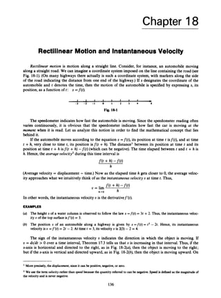
![CHAP. 181 RECTILINEAR MOTION AND INSTANTANEOUS
the other hand, if U = ds/dt -c0 over a time interval, then s must be
137
VELOCITY
decreasing in that interval. In
Fig. 18-2(a),the object would be moving to the left (in the direction of decreasing s);in Fig. 18-2(b),the
object would be moving downward.
A consequence of these facts is that at an instant t when a continuously mooing object reverses
direction, its instantaneous oelocity o must be 0. For if U were, say, positive at t, it would be positive in a
small interval of time surrounding t ; the object would therefore be moving in the same direction just
before and just after t. Or, to say the same thing in a slightly different way, a reversal in direction means
a relative extremum of s, which in turn implies (Theorem 14.1)ds/dt = 0.
EXAMPLE An object moves along a straight line as indicated in Fig. 18-3(a).In functional form,
s = f ( t ) = (t +2)2 [s in meters, t in seconds]
as graphed in Fig. 18-3(b).The object’s instantaneous velocity is
t, =f’(t) = 2(t +2) [meters per second]
For t +2 < 0, or t < -2, o is negative and the object is moving to the left; for t +2 > 0, or t > -2, t, is positive
and the object is moving to the right. The object reverses direction at t = -2, and at that instant U = 0. [Note that
f ( t )has a relative minimum at t = -2.1
t = -3 t = - 4
(--------
+
0 S
-*--- +-a----
I = -0.5 I = 0 I = I
Free Fall
(b)
Fig. 18-3
Consider an object that has been thrown straight up or down, or has been dropped from rest, and
which is acted upon solely by the gravitational pull of the earth. The ensuing rectilinear motion is called
jieefall.
Let us put a coordinate system on the vertical line along which the object moves, such that the
s-axis is directed upward, away from the earth, with s = 0 located at the surface of the earth (Fig. 18-4).](https://image.slidesharecdn.com/problemscalculus-221128025033-038ef06f/85/problems-calculus-pdf-150-320.jpg)
![CHAP. 181 RECTILINEAR MOTION AND INSTANTANEOUS VELOCITY 141
The car is never at rest. It makes sense to talk about the car being at rest only when the position of the
car is constant over an interval of time (not at just a single point). In such a case, the velocity would be zero
on an entire interval.
Supplementary Problems
18.4 (a) If an object is released from rest at any given height, show that, after t seconds, it has dropped 16t2feet
(assumingthat it has not yet struck the ground).
(b) How many seconds does it take the object in part (a)to fall: (i) 1 foot; (ii) 16feet; (iii)64 feet; (iv) 100
feet?
185 A rock is dropped down a well that is 256 feet deep. When will it hit the bottom of the well?
18.6 Assuming that one story of a building is 10feet, with what speed, in miles per hour, does an object dropped
from the top of a 40-story building hit the ground?
A rocket is shot straight up into the air with an initial velocity of 128feet per second.
(a)How far has it traveled in 1 second? in 2 seconds? (b) When does it reach its maximum height? (c)What
is its maximum height? (d) When does it hit the ground again? (e) What is its speed when it hits the
ground ?
18.7
18.8 A rock is thrown straight down from a height of 480 feet with an initial velocity of 16feet per second.
(a)How long does it take to hit the ground? (b) With what speed does it hit the ground? (c) How long does
it take before the rock is moving at a speed of 112 feet per second? (d)When has the rock traveled a
distance of 60feet?
3
An automobile moves along a straight highway, with its position given by s = 12t3- 18t2+9t --
2
[s in miles, t in hours].
(a) Describe the motion of the car: when it is moving to the right, when to the left, where and when it
changes direction.
(b) What distance has it traveled in 1 hour from t = 0 to t = l ?
18.9
18.10 The position of a moving object on a line is given by the formula s = (t - l)3(t - 5).
(a) When is the object moving to the right? (b) When is it moving to the left? (c) When is it changing
direction? (d) When is it at rest? (e)What is the farthest to the left of the origin that it moves?
18.11 A particle moves on a straight line so that its position s (miles) at time t (hours) is given by
(a) When is the particle moving to the right? (b)'When is the particle moving to the left? (c) When does it
change direction? (d)When the particle is moving to the left, what is the maximum speed that it achieves?
(The speed is the absolute value of the velocity.)
s = (4t - 1Kt - 1)2.
18.12 A particle moves along the x-axis according to the equation x = 10t - 2t2. What is the total distance
covered by the particle between t = 0 and t = 3?
18.13 A rocket was shot straight up from the ground. What must have been its initial velocity if it returned to
earth in 20 seconds?](https://image.slidesharecdn.com/problemscalculus-221128025033-038ef06f/85/problems-calculus-pdf-154-320.jpg)
![Chapter 19
Instantaneous Rate of Change
One quantity, y, may be related to another quantity, x, by a functionf: y =f(x). A change in the
value of x usually induces a corresponding change in the value of y.
EXAMPLE Let x be the length of the side of a cube, and let y be the volume of the cube. Then y = x3.In the case
where the side has length x = 2 units, consider a small change Ax in the length.
NOTATION Ax (read “delta-ex”) is the traditional symbol in calculus for a small change in x. Ax is considered a
single symbol, not a product of A and x. In earlier chapters, the role of Ax often was taken by the symbol h.
The new volume will be (2 +Ax)~,
and so the change in the value of the volume y is (2 +A x ) ~
- Z3. This change in
y is denoted traditionally by Ay,
Ay = (2 +A x ) ~
- 23
Now the natural way to compare the change Ay in y to the change Ax in x is to calculate the ratio Ay/Ax. This
ratio depends of course on Ax, but if we let Ax approach 0, then the limit of Ay/Ax will define the instantaneousrate
o
f change of y compared to x, when x = 2. We have (ALGEBRA, Problem 11.2)
Ay = (2 +A x ) ~
-23 = [(2)3+3(2)2(A~)1
+3(2)’(A~)~
+(Ax)~]- 23
= 1 2 6 ~
+~ ( A x ) ~
+(Ax)~= (AxX12 +6Ax +(Ax)~)
Hence, --
Ay - 12 +6Ax +(Ax)’
Ax
and AY
lim -= lim (12 + 6Ax +(AX)~)
= 12
Ax-0 Ax Ax+O
Therefore, when the side is 2, the rate of change of the volume with respect to the side is 12. This means that, for
sides close to 2, the change Ay in the volume is approximately 12 times the change Ax in the side (since Ay/Ax is
close to 12).Let us look at a few numerical cases.
If Ax = 0.1, then the new side x +Ax is 2.1, and the new volume is (2.1)3= 9.261. So, Ay = 9.261 - 8 = 1.261,
and
Ay 1.261
Ax 0.1
----= 12.61
If Ax = 0.01, then the new side x +Ax is 2.01, and the new volume is (2.01)3= 8.120601. So,
Ay = 8.120601 -8 = 0.120601, and
12.0601
Ay 0.120601
Ax 0.01
-=-=
If Ax = 0.001, a similar computation yields
--
Ay - 12.006001
Ax
Let us extend the result of the above example from y = x3 to an arbitrary differentiable function
y =f(x). Consider a small change Ax in the value of the argument x. The new value of the argument is
143](https://image.slidesharecdn.com/problemscalculus-221128025033-038ef06f/85/problems-calculus-pdf-156-320.jpg)
![CHAP. 191
When r = 10,
INSTANTANEOUS RATE OF CHANGE
-=
dV 4n(10)’ = 4OOn w 400(3.14) = 1256
dr
4 4000n
3 3
4 4 4121.204~
3 3
~ ( 1 0 )
= - 410)3 = -
3
V(lO.1) = -~(10.1)~
= - lt(1030.301) =
4121.204~ 4 0 0 0 ~
--
3 3
AV = V(10.1) - V(10) =
n R 3.14
3 3 3
= - (4121.204 - 4ooo) = - (121.204) w -(121.204)
= 126.86 cubic millimeters
The change predicted from (29.2)and part (a)is
145
dV
dr
AV x -Ar = 125qO.l) = 125.6cubic millimeters
19.3 An oil tank is being filled. The oil volume V ,in gallons, after t minutes is given by
V = 1.W +2t
How fast is the volume increasing when there is 10 gallons of oil in the tank? [Hint: To answer
the question, “how fast?,” you must always find the derivative with respect to time.]
When there are 10gallons in the tank,
1 3 ’ +2t = 10 or 1.9’ +2t - 10 = 0
Solvingby the quadratic formula,
-2 f ,/4 - 4(1.5K-10) -2 k , / 4 3 -2 f@ -2 +8 10
-
- -
- =
:
=
2 or --
3 3 3 3
t =
2(1.5)
Since t must be positive, t = 2 minutes. The rate at which the oil volume is growing is
dV
dt
-= D,(1.5t2 +2t) = 3t +2
Hence, at the instant t = 2 minutes when V = 10gallons,
--- 3(2) +2 = 6 + 2 = 8 gallons per minute
dV
dt
Supplementary Problems
19.4 The cost C, in dollars per day, of producing x TV sets per day is given by the formula
C = 7000 +5 0 ~
- 0 . 0 5 ~ ~
Find the rate of change of C with respect to x (called the marginal cost) when 200 sets are being produced
each day.](https://image.slidesharecdn.com/problemscalculus-221128025033-038ef06f/85/problems-calculus-pdf-158-320.jpg)
![146 INSTANTANEOUS RATE OF CHANGE [CHAP. 19
19.5 The profit P, in dollars per day, resulting from making x units per day of an antibiotic, is
P = 5x +0.02x2- 120
Find the marginal profit when the production level x is 50 units per day.
19.6 Find the rate at which the surfacearea of a cube of side x is changing with respect to x, when x = 2 feet.
19.7 The number of kilometers a rocket ship is from earth is given by the formula
E = 30t +0.005t2
where t is measured in seconds. How fast is the distance changing when the rocket ship is 35000 kilometers
from earth?
19.8 As a gasoline tank is being emptied, the number G of gallons left after t seconds is given by G = 3(15 - t)2.
(a) How fast is gasoline being emptied after 12seconds? (b) What was the average rate at which the gasoline
was being drained from the tank over the first 12 seconds? [Hint: The average rate is the total amount
emptied divided by the time during which it was emptied.]
19.9 If y = 3x2-2, find: (a) the average rate at which y changes with respect to x over the interval [1, 21; (b)
the instantaneous rate of change of y with respect to x when x = 1.
19.10 If y =f(x) is a function such thatf’(x) # 0 for any x, find those values of y for which the rate of increase of
y4 with respect to x is 32 times that of y with respect to x.](https://image.slidesharecdn.com/problemscalculus-221128025033-038ef06f/85/problems-calculus-pdf-159-320.jpg)
![148 RELATED RATES [CHAP. 20
In Fig. 20-1, ASMN and ASAL are similar, whence
Y 6
S M N M
__ - or ---
SA LA y + x 15
-
-=-
which is the desired relation between x and y. In this case, it is convenient to solve (1)for y in terms of x,
--
Y 2
--
y + x 5
5y = 2y +2x
3y = 2x
2
3
y = - x
Differentiation of (2)with respect to t gives
dy 2 dx
- = - -
dt 3 dt
(3)
Now because the man is running away from A at the rate of 18 feet per second, x is increasing at that rate.
Hence,
dx
-= 18 feet per second
dt dt 3
and -
dy = -(18) = 12 feet per second
that is, the shadow is lengthening at the rate of 12 feet per second.
(b) A cube of ice is melting. The side s of the cube is decreasing at the constant rate of 2 inches per minute. How
fast is the volume V decreasing?
Since V = s3,
ds
dt dt dt
[by the power chain rule]
d V 4s’) - 3s2 -
-=--
The fact that s is decreasing at the rate of 2 inches per minute translates into the mathematical statement
ds
dt
--
- -2
d V
dt
-= 3s2(-2) = -6s2
Hence,
Thus, although s is decreasing at a constant rate, V is decreasing at a rate proportional to the square of s. For
instance, when s = 3 inches, V is decreasing at a rate of 54 cubic inches per minute.
(c) Two small airplanes start from a common point A at the same time. One flies east at the rate of 300 kilometers
per hour and the other flies south at the rate of 400 kilometers per hour. After 2 hours, how fast is the distance
between them changing?
Refer to Fig. 20-2. We are given that dx/dt = 300 and dy/dt = 400 and wish to find the value of du/dt at
t = 2 hours. The necessary relation between U,x, and y is furnished by the Pythagorean theorem,
U2 = x2 +y2
Therefore,
d(u2) d(x2 +y2)
-- -
dt dt
du d(x2) d(y2)
2u-=-+-
dt dt dt
[by the power chain rule]
du dx
2u -= 2x -+2y -
dy
dt dt dt
du dx dy
dt dt dt
[by the power chain rule]
U -= x -+y -= 300x +400y](https://image.slidesharecdn.com/problemscalculus-221128025033-038ef06f/85/problems-calculus-pdf-161-320.jpg)

![152 RELATED RATES
0
0
0
/
0
0
0
0
;0‘
0
0
/
/
0
0
0
0
0
0
0
r
,
[CHAP. 20
S
and, by (0
U = JM
= JZGTZZi = ,/Z@= 52
Substitution in (2)yields
du
dt
52 = -12(48)+ lO(20) = -576 +200 = -376
x -7.23
du 376
dt 52
--
- --
which shows that, after 2 hours, the distance between ships B and C is decreasing at the rate of 7.23 knots.
Supplementary Problems
20.5 The top of a 25-foot ladder, leaning against a vertical wall, is slipping down the wall at the rate of 1foot per
minute. How fast is the bottom of the ladder slipping along the ground when the bottom of the ladder is 7
feet away from the base of the wall?
20.6 A cylindrical tank of radius 10feet is being f
i
l
l
e
d with wheat at the rate of 314 cubic feet per minute. How
fast is the depth of the wheat increasing? [Hint: The volume of a cylinder is nr2h,where r is its radius and h
its height.]
20.7 A 5-fOOt girl is walking toward a 20-foot lamppost at the rate of 6 feet per second. How fast is the tip of her
shadow (cast by the lamp) moving?
20.8 A rocket is shot vertically upward with an initial velocity of 400 feet per second. Its height s after t seconds
is s = 400t - 16t2. How fast is the distance between the rocket and an observer on the ground 1800 feet
away from the launching site changing when the rocket is still rising and is 2400 feet above the ground (see
Fig. 20-6)?
Fig. 20-6
20.9 A small funnel in the shape of a cone is being emptied of fluid at the rate of 12cubic millimetersper second.
The height of the funnel is 20 millimeters and the radius of the base is 4 millimeters. How fast is the fluid
level dropping when the level stands 5 millimeters above the vertex of the cone? [Remember that the
volume of a cone is 3nr’h.I](https://image.slidesharecdn.com/problemscalculus-221128025033-038ef06f/85/problems-calculus-pdf-165-320.jpg)
![CHAP. 201 RELATED RATES 153
20.10
20.11
20.12
20.13
20.14
20.15
20.16
20.17
20.18
20.19
20.20
A balloon is being inflated by pumping in air at the rate of 2 cubic inches per second. How fast is the
diameter of the balloon increasingwhen the radius is one-half inch?
Oil from an uncapped oil well in the ocean is radiating outward in the form of a circular film on the surface
of the water. If the radius of the circle is increasing at the rate of 2 meters per minute, how fast is the area of
the oil film growingwhen the radius reaches 100meters?
The length of a rectangle having a constant area of 800 square millimeters is increasing at the rate of 4
millimeters per second.(a)What is the width of the rectangle at the moment when the width is decreasing at
the rate of 0.5 millimeter per second? (b) How fast is the diagonal of the rectangle changing when the width
is 20 millimeters?
A particle moves on the hyperbola x2 - 18y2= 9 in such a way that its y-coordinate increases at a constant
rate of nine units per second. How fast is its x-coordinate changing when x = 9?
An object moves along the graph of y =f(x). At a certain point, the slope of the curve (that is, the slope of
the tangent line to the curve) is 3 and the abscissa (x-coordinate) of the object is decreasing at the rate of
three units per second. At that point, how fast is the ordinate (y-coordinate)of the object changing? [Hint:
y =f(x), and x is a function oft. So y is a composite function oft, which may be differentiated by the chain
rule.]
If the radius of a sphere is increasingat the constant rate of 3 millimeters per second, how fast is the volume
changing when the surface area (4ar2)is 10square millimeters?
What is the radius of an expanding circle at a moment when the rate of change of its area is numerically
twice as large as the rate of change of its radius?
A particle moves along the curve y = 2x3 - 3x2 +4. At a certain moment, when x = 2, the particle’s
x-coordinate is increasing at the rate of 0.5 unit per second. How fast is its y-coordinate changing at
that moment?
A plane flying parallel to the ground at a height of 4 kilometers passes over a radar station R (see Fig. 20-7).
A short time later, the radar equipment reveals that the plane is 5 kilometers away and that the distance
between the plane and the station is increasing at a rate of 300 kilometers per hour. At that moment, how
fast is the plane moving horizontally?
A boat passes a fixed buoy at 9 A.M.,heading due west at 3 miles per hour. Another boat passes the same
buoy at 10A.M.,heading due north at 5 miles per hour. How fast is the distance between the boats changing
at 11:30A.M.?
Water is pouring into an inverted cone at the rate of 3.14 cubic meters per minute. The height of the cone
is 10 meters and the radius of its base is 5 meters. How fast is the water level rising when the water stands
7.5 meters in the cone?
R
Fig. 20-7 Fig. 20-8](https://image.slidesharecdn.com/problemscalculus-221128025033-038ef06f/85/problems-calculus-pdf-166-320.jpg)
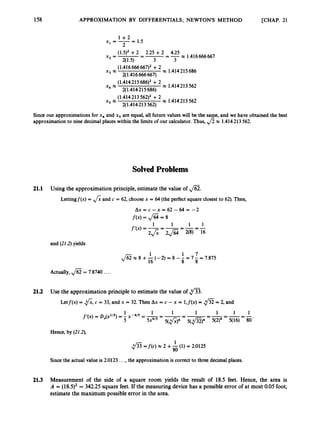
![CHAP. 211 APPROXIMATION BY DIFFERENTIALS ; NEWTONS METHOD 159
The formula for the area is A = x2, where x is the side of the room. Hence, dA/dx = 2x. Let x = 18.5,
and let 18.5 +Ax be the true length of the side of the room. By assumption, IAxl I 0.05. The approx-
imation principle yields
dA
dx
A(x +Ax) -A(x) x -AX
A(18.5 +Ax) - 342.25 x q18.5) AX
IA(18.5 +Ax) - 342.25 I x I37 Ax I I
37(0.05) = 1.85
Hence, the error in the area should be at most 1.85 square feet, putting the actual area in the range of
(342.25 +_ 1.85) square feet. See Problem 21.13.
21.4 Use Newton’s method to find the positive solutions of
x 4 + x - 3 = 0
Let f(x) = x4 +x - 3. Then f’(x) = 4x3 +1. Since f(1) = -1 and f(2) = 15, the intermediate-value
theorem tells us that there is a solution between 1and 2. [The interval (1, 2) is suggested by drawing the
graph off with a graphing calculator.] Sincef’(x) > 0 for x 2 0,f is increasing for x >0, and, therefore,
there is exactly one positive real solution. Start with xo = 1.Equation (22.5) becomes
x
: +x
, - 3 4x: +x, - (x: +x
, - 3) 3x: +3
4 4 + 1 4x,3 + 1 4x: + 1
--
-
-
-
= X n -
Successive calculations yield x1 = 1.2, x2 = 1.165419616, x3 = 1.164037269, xq = 1.164035 141, and
x5 = 1.164035 141.Thus, the approximate solution is x = 1.164035 141.
21.5 Show that if Newton’s method is applied to the equation x113= 0 with xo = 1, the result is a
divergentsequence of values (which certainlydoes not converge to the root x = 0).
1
3X2l3
Letf(x) = x’/~.
So,f’(x)= -and (22.5) becomes
x,+1 = x
, - -
= x, - 3x, = -2x,
1/(3x,213)
Hence, x1 = -2, x2 = 4, x3 = -8, and, in general, x, = (-2)”.
Note: If we are seeking a solution r of an equation f(x) = 0, then it can be shown that a sufficient
condition that Newton’s method yields a sequence of values tht converges to r is that
for all x in an interval around r that includesxo.However, this is not a necessary condition.
SupplementaryProblems
21.6 Use the approximation principle to estimate the followingquantities:
(a) f i (b) ,/% (c) .
@ (d) (8.35)2/3 (e) (33)-’/’
(f) & (g) diE5 (h) Jsos (i) f l](https://image.slidesharecdn.com/problemscalculus-221128025033-038ef06f/85/problems-calculus-pdf-172-320.jpg)
![160
21.7
21.8
21.9
21.10
21.11
21.12
21.13
21.14
21.15
21.16
21.17
21.18
21.19
21.20
APPROXIMATION BY DIFFERENTIALS; NEWTONS METHOD [CHAP. 21
The measurement of the side of a cubical container yields 8.14 centimeters, with a possible error of at most
0.005 centimeter. Give an estimate of the maximum possible error in the value of V = (8.14)3= 539.353 14
cubic centimeters for the volume of the container.
It is desired to give a spherical tank 20 feet (240 inches) in diameter a coat of paint 0.1 inch thick. Use the
approximation principle to estimate how many gallons of paint will be required. (V = 41cr3, and 1 gallon is
about 231 cubic inches.)
A solid steel cylinder has a radius of 2.5 centimeters and a height of 10 centimeters. A tight-fitting sleeve is
to be made that will extend the radius to 2.6 centimeters. Find the amount of steel needed for the
sleeve: (a)by the approximation principle; (b) by an exact calculation.
If the side of a cube is measured with a percentage error of at most 3%, estimate the maximum percentage
error in the volume of the cube. (If AQ is the error in measurement of a quantity Q, then IAQ/Q I x 100% is
the percentage error.)
Assume, contrary to fact, that the Earth is a perfect sphere, with a radius of 4000 miles. The volume of ice at
the North and South Poles is estimated to be about 8000000 cubic miles. If this ice were melted and if the
resulting water were distributed uniformly over the globe, approximately what would be the depth of the
added water at any point of the Earth?
(a) Let y = x3/2.When x = 4 and dx = 2, find the value of dy.
(b) Let y = 2 x , / m ’ . When x = 0 and dx = 3, find the value of dy.
For Problem 21.3, calculate exactly the largest possible error in the area.
Establish the very useful approximation formula (1 +U
)
’ x 1 +ru, where r is any rational exponent and Iu I
is small compared to 1. [Hint: Apply the approximation principle tof(x) = x
‘
, letting x = 1and Ax = u.]
Use Newton’s method to approximate the followingquantities:
Show that Newton’s method for finding 4yields the equation
for the sequence of approximating values.
Use part (a)to approximate fi by Newton’s method.
Use Newton’s method to approximate solutions of the following equations:
x3 - x - 1 = 0 (b) x3 +x - 1 = 0 (c) x4 - 2 ~ ’
+0.5 = 0 (d) x3 +2~ - 4 = 0
x 3 - 3 x 2 + 3 = o (f) x 3 - x + 3 = 0 (9) x 3 - 2 x - 1 = 0
Show that x3 +x2 - 10 = 0 has a unique root in (1, 2) and approximate this root by Newton’s method,
with xo = 2.
Show that xs +5x - 7 = 0 has a unique solution in (1,2) and approximate this root by Newton’s method.
Explain why Newton’s method does not work in the following cases:
(a) Solvex3 - 6x2+ 12x - 7 with xo = 2.
(b) Solve x3 - 3x2 +x - 1 = 0 with xo = 1.
Jx-1 f o r x 2 1
(c) Solvef(x) = 0, wheref(x) = and xo > 1 (say, x = 1 +b, b > 0
)
.](https://image.slidesharecdn.com/problemscalculus-221128025033-038ef06f/85/problems-calculus-pdf-173-320.jpg)
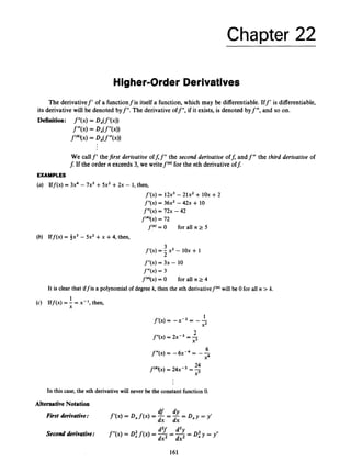
![162 HIGHER-ORDER DERIVATIVES [CHAP. 22
d3f d3y
f’”(X) = 0,”
f(x) = -- -= D,”y y”t
f (“)(x)= 0
; f(x) = -
d”f -
--
‘“Y -
- D;y = y(n)
dx3 -dx3
dx” dx”
Third derivative:
nth derivative:
Higher-Order ImplicitDifferentiation
EXAMPLE Let y = f ( x ) be a differentiablefunctionsatisfyingthe equation
x2 +yz = 9
(we know that y = ,
/
=
or y = -
,
/
-
; their graphs are shown in Fig. 22-1.)
Let us find a formula for the second derivativey”, where y stands for either of the two functions.
DJx2 +y2)= Dx(9)
x +yy’ = 0
2x +2yy’ = 0 [D,y2 = 2yy’ by the power chain rule]
Next, differentiateboth sidesof (I)with respect to x,
Dx@+YY’) = DX(0)
1 +yD#) +y’Dxy = 0
1 +yy” +y‘ y’ = 0
1 +yy” +(y’y = 0
Solve(I)for y’ in terms of x and y,
Substitute -(x/y) for y’ in (2),
X*
Y
1 +yy” +2= 0
y2 +y3y” +x2 = 0 [multiplying by y2]
Solvefor y”,
t’
(a) y = d9- x! (b) y = -v9- x!
Fig. 22-1](https://image.slidesharecdn.com/problemscalculus-221128025033-038ef06f/85/problems-calculus-pdf-175-320.jpg)
![164 HIGHER-ORDER DERIVATIVES [CHAP. 22
( x + l)D,X - xD,(x + 1)
( x + 1)2
(4 f”x) = [by the quotient rule]
1
-
--
= ( x + 1)-2
( X + 1x1)- ~ ( 1 )
- x + 1 - x
-
-
-
( x + 1)2 (x + 1)2 ( x +
f y x ) = -2(x + 1 ) - 3 ~ , ( ~
+ 1) [by the power chain rule]
~~
ALGEBRA (-1y-l will be 1 when n is odd and -1 when n is even. n! stands for the product
1 x 2 x 3 x - - - x n of the first n positive integers.
22.2 Find y” if
y3 - xy = 1 (0)
Differentiation of(0), using the power chain rule for D,y3 and the product rule for D,(xy), gives
3y2y’ - (xy’ +y) = 0
3y2y’ - xy‘ - y = 0
(3y2 - x)y’ - y = 0
Next, differentiate(Z),
(3y2 - x)D,y’ +y’D,(3y2 - x) - y’ = 0
(3y2 - x)y” +y’(6yy’ - 1)- y’ = 0
(3y2- x)y” +y’((6yy’ - 1)- 1) = 0
[by the product rule]
[by the power chain rule]
[factor y’]
(3y2- X)Y” +y’(6yy’ - 2) = 0
Now solve(1)for y‘,
Y
y’ = -
3y2 - x
Finally, substitute into (2)and solve for y”,
(3y2 - x)y” + +
L (K
- 2) = 0
3y - x 3y2 - x
(3y2 - X)~Y’’ +(3y2 - x ) 7
Y (3y2 - x)(- 6Y - 2 ) = 0 [multiply by (3y2 - x ) ~ ]
3y - x 3y2 - x
(3y2- X)~Y’’
+y (6y2 - 2(3y2 - x)) = 0 [U(: - c ) = b - cu]
(3y2 - x ) ~ Y ”
+v(6v2- 6y2 +2 ~ )0
(3y2 - x)3y” +2xy = 0
-2xy
(3y2 - x)3
y” =](https://image.slidesharecdn.com/problemscalculus-221128025033-038ef06f/85/problems-calculus-pdf-177-320.jpg)
![CHAP. 221 HIGHER-ORDER DERIVATIVES 165
2
2
.
3 If y is a function of x such that
x3 - 2xy +y3 = 8 (0)
and such that y = 2 when x = 2 [note that these values satisfy (O)], find the values of y’ and y”
when x = 2.
Proceed as in Problem 22.2.
x3 - 2xy +y3 = 8
D,(x3 - 2xy +y3)= D,(8)
3x2 - 2(xy’ +y) +3y2y’ = 0
3x2 -2xy’ - 2y +3y2y’ = 0
DX(3X2- 2xy’ - 2y +3y2y’) = D,(O)
6~ - ~(XY’’
+y’) - 2y’ +3dy’y’‘ +y’(2yy’)) = 0
6~ - 2xy” - 2y’ - 2y’ +3y2y” +6 ~ 4 ~ ’ ) ~
= 0
Substitute 2 for x and 2 for y in (I),
Substitute 2 for x, 2 for y, and -1for y’ in (2),
28 7
y”= -T= - -
2
12 - 4y” +2 +2 + 12y” + 12 = 0 or 8y” +28 = 0 or
22.4 Let s = t3 - 9t2 +24t describe the position s at time t of an object moving on a straight line.
(a)Find the velocity and acceleration. (b) Determine when the velocity is positive and when it is
negative. (c) Determine when the acceleration is positive and when it is negative. (6)Describe the
motion of the object.
ds
dt
U = - = 3t2 - 18t +24 = 3(t2- 6t +8) = 3(t -2Xt - 4)
dv
dt
a = - = 6t - 18 = 6(t - 3)
U is positive when t - 2 > 0 and t - 4 > 0 or when t - 2 < 0 and t - 4 < 0; that is, when
t > 2 and t > 4 or t < 2 and t <4
which is equivalent to t > 4 or t < 2. v = 0 if and only if t = 2 or t = 4. Hence, U <0 when 2 < t < 4.
a > Owhen t > 3, and a <Owhen t < 3.
Assuming that s increases to the right, positive velocity indicates movement to the right, and negative
velocity movement to the left. The object moves right until, at t = 2, it is at s = 20, where it reverses
direction. It then moves left until, at t = 4, it is at s = 16, where it reverses direction again. Thereafter,
it continues to move right (see Fig. 22-2).
Fig. 22-2](https://image.slidesharecdn.com/problemscalculus-221128025033-038ef06f/85/problems-calculus-pdf-178-320.jpg)
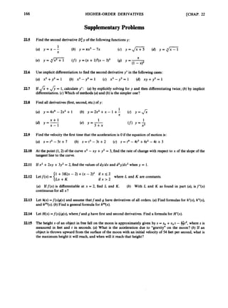
![Chapter 23
Applications of the Second Derivative and
Graph Sketching
2
3
.
1 CONCAVITY
If a curve has the shape of a cup or part of a cup (like the curves in Fig. 23-l), then we say that it is
concuue upward. (To remember the sense of “concave upward,” notice that the letters c and up form the
word cup.) A mathematical description of this notion can be given. A curve is concave upward if the
curve lies above the tangent line at any given point of the curve. Thus, in Fig. 23-l(a) the curve lies
above all three tangent lines.
/
/
/
/
Fig. 23-1 Concavity *ward
A curve is said to be concavedownwardif it has the shape of a cap or part of a cap (see Fig. 23-2).In
mathematical terms, a curve is concave downward if it lies below the tangent line at an arbitrary point
of the curve [see Fig. 23-2(a)].
(4 (b)
Fig. 23-2 Concavity downward
A curve may, of course, be composed of parts of different concavity. The curve in Fig. 23-3 is
concave downward from A to B, concave upward from B to C, concave downward from C to D, and
concave upward from D to E. A point on the curve at which the concavitychanges is called an inflection
point. B, C, and D are inflectionpoints in Fig. 23-3.
167](https://image.slidesharecdn.com/problemscalculus-221128025033-038ef06f/85/problems-calculus-pdf-180-320.jpg)
![168 THE SECOND DERIVATIVE AND GRAPH SKETCHING [CHAP. 23
Fig. 23-3
From Fig. 23-1 we see that if we move from left to right along a curve that is concave upward, the
slope of the tangent line increases. The slope either becomes less negative or more positive. Conversely,
if the tangent line has this property, the curve must be concave upward. Now for a curve y =f(x), the
tangent line will certainly have this property iff”(x) > 0 since, in that case, Theorem 17.3 implies that
the slopef’(x) of the tangent line will be an increasing function. By a similar argument, we see that if
f”(x)< 0, the slope of the tangent line is decreasing, and from Fig. 23-2 we see that the curve y = f ( x ) is
concavedownward. This yields:
Theorem 2
3
.
l
: Iff”(x) > 0 for all x in (a, b), then the graph off is concave upward between x = a and
x = b. Iff”(x) <0 for all x in (a, b), then the graph offis concave downward between
x = a and x = b.
For a rigorous proof of Theorem 23.1, see Problem 23.17.
Corollary2
3
.
2
: If the graph off has an inflection point at x = c, and f”exists and is continuous at
x = c, then$”@)= 0.
In fact, if f”(c) # 0, the f”(c) > 0 or f”(c) < 0. If f”(c) > 0, then f”(x)> 0 for all x in some open
interval containing c, and the graph would be concave upward in that interval, contradicting the
assumption that there is an inflection point at x = c. We get a similar contradiction iff”(c) <0, for in
that case, the graph would be concavedownward in an open interval containing c.
EXAMPLES
(a) Consider the graph of y = x3 [see Fig. 23-4(a)]. Here y’ = 3x2 and y” = 6x. Since y” > 0 when x > 0, and
y” < 0 when x < 0, the curve is concave upward when x > 0, and concave downwardwhen x <0. There is an
inflection point at the origin, where the concavity changes. This is the only possible inflection point, for if
y” = 6x = 0, then x must be 0.
(b) Iff”(c) = 0, the graph offneed not have an inflection point at x = c. For instance, the graph off($ = x4 [see
Fig. 23-4(b)] has a relative minimum, not an inflection point, at x = 0, wheref”(x) = 12x2= 0.
Fig. 23-4](https://image.slidesharecdn.com/problemscalculus-221128025033-038ef06f/85/problems-calculus-pdf-181-320.jpg)
![CHAP. 231 THE SECOND DERIVATIVE AND GRAPH SKETCHING 169
23.2 TEST FOR RELATIVE EXTREMA
We already know, from Chapter 14, that the conditionf'(c) = 0 is necessary, but not sufficient, for a
differentiable function f to have a relative maximum or minimum at x = c. We need some additional
information that will tell us whether a function actually has a relative extremum at a point where its
derivative is zero.
Theorem 2
3
.
3 (Second-Derivative Test for Relative Extrema): If f'(c) = 0 and f"(c) < 0, then f has a
relative maximum at c. Iff'(c) = 0 andf"(c) > 0, thenfhas a relative minimum at c.
Proof: Iff'(c) = 0, the tangent line to the graph off is horizontal at x = c. If, in addition,f"(c) -c0,
then, by Theorem 23.1,' the graph off is concave downward near x = c. Hence, near x = c, the graph
off must lie below the horizontal line through (c,f(c));f thus has a relative maximum at x = c [see
Fig. 23-5(a)].A similar argument leads to a relative minimum whenf"(c) > 0 [see Fig. 23-5(b)].
I
I I
I I
C C
I 1
EXAMPLE Consider the functionf(x) = 2x3 +x2 - 4x +2. Then,
f'(x)=
r 6x2 +2x - 4 = 2(3x2 +x -2) = 2(3x -2Xx + 1)
Hence, iff'(x) = 0, then 3x - 2 = 0 or x + 1 = 0;that is, x = 3 or x = -1. Nowf"(x) = 12x +2. Hence,
f"(-1) = 12(-1) +2 = -12 +2 = -10 < 0
f''(4) = 12(3) +2 = 8 +2 = 10 > 0
Fig. 23-6
In order to use Theorem 23.1, we must assume thatf" i
s continuous at c and exists in an open interval around c. However,a
more complicatedargumentcan avoid that assumption.](https://image.slidesharecdn.com/problemscalculus-221128025033-038ef06f/85/problems-calculus-pdf-182-320.jpg)
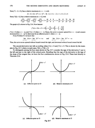
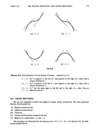
![172 THE SECOND DERIVATIVE AND GRAPH SKETCHING [CHAP. 23
EXAMPLE Sketch the graph of the rational function
X
f(x) = -
x2 + 1
First of all, the function is odd [that is,f(-x) = -f(x)], so that it need be graphed only for positive x. The
Compute the first two derivativesoff,
graph is then completed by reflection in the origin (seeSection 7.3).
(x’ + ~)D,(x)- xD,(x2 + 1) x2 + 1 - x(~x) 1 - X’
=-
-
-
f‘(4= (x2+ 1)2 (x2+ 1)2 (x2+ 1)2
(x2+ 1)2Dx(1
- x2)- (1 - x2)D,((x2 + 1)2)
(x2 + 1)4
f”(x) = Dxf’(x) =
- (x’ + 1)2(-2~)
- (1 - x2)[2(x2+ 1)(2~)]
-
(x2 + 114
-2x(x2 + 1)[x2 + 1 +2(1 - x2)] -2x(3 - x2)- 2x(x - &)(x +&)
-
-
-
-
-
(x2 + 114 (x2 + 1)3 (xz + 113
Since 1 -x2 = (1 - xX1 +x), f’(x) has a single positive root, x = 1, at which f”(1) = [-2(2)]/(2)3 = -4.
If we examine the formula forf”(x),
Hence, by the second-derivativetest,fhas a relative maximum at x = 1.The maximum value isf(1) = #.
~ X ( X
- J3Xx +J3)
f“(x)=
(x2 + 113
we see that f”(x) > 0 when x > fi and that f”(x) -c0 when 0 < x < fi.By Theorem 23.1, the graph off
is concave upward for x > & and concave downward for 0 < x < fi.Thus, there is an inflection point I at
x = &,where the concavity changes.
Now calculate
-0
0
llX - -
X
lim f(x) = lim --
- lim
x + + w X’+a) x2 + 1 X‘+W 1 +(1/x2) 1 +0
which shows that the positive x-axis is a horizontal asymptote to the right.
The graph, with its extension to negative x (dashed),is sketched in Fig. 23-9. Note how concavity of one kind
reflects into concavity of the other kind. Thus, there is an inflectionpoint at x = -&and another inflection point
at x = 0. The valuef(1) = # is the absolute maximum off, andf( -1)= -4 is the absolute minimum.
Fig. 23-9](https://image.slidesharecdn.com/problemscalculus-221128025033-038ef06f/85/problems-calculus-pdf-185-320.jpg)
![CHAP. 231 THE SECOND DERIVATIVE AND GRAPH SKETCHING 173
Solved Problems
2
3
.
1 Sketch the graph off@) = x - l/x.
The function is odd. Hence, we can first sketch the graph for x > 0 and, later, reflect in the origin to
The first and second derivativesare
obtain the graph for x < 0.
I
1
X2
f ' ( x ) = D , ( x - X - ' ) = l - ( - l ) x - 2 = 1 + -
2
fryx) = ~ ~ ( 1
+ x-2) = -2x-3 = - -
x3
Sincef'(x) = 1+(l/xz) > 0,fis an increasing function. Moreover, for x > 0, the graph off is concave
downward, sincef"(x) = -(2/x3) < 0 when x > 0. The line y = x turns out to be an asymptote, because
1
X - + m x + + m x
lim [x -f(x)] = lim - = 0
Since
the graph offhas the negative y-axis as a vertical asymptote.
Notice that x = 0, at whichfis undefined,is the only critical number. The graph is sketched, for all x,
in Fig. 23-10. Although the concavity changes at x = 0, there is no inflection point there becausef(0) is not
defined.
6 C
I L X
(-1. -i)
Fig. 23-10 Fig. 23-11](https://image.slidesharecdn.com/problemscalculus-221128025033-038ef06f/85/problems-calculus-pdf-186-320.jpg)
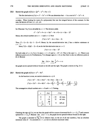
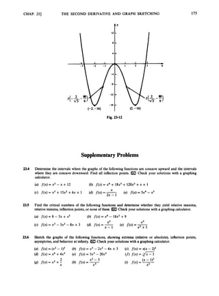
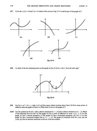
![CHAP. 23) THE SECOND DERIVATIVE AND GRAPH SKETCHING 1I7
23.11
23.12
23.13
23.14
23.15
23.16
23.17
23.18
23.19
Iff(x) = x3 +3x2 +k has three distinct real roots, what are the bounds on k? [Hint: Sketch the graph off;
usingf’ andf”. At how many points does the graph cross the x-axis?]
Sketch the graph of a continuous functionfsuch that:
(a) f(1) = -2,f‘( 1)= O,f”(x) > 0 for all x
(6) f(2) = 3,f’(2) = O,f”(x) <0 for all x
(c) f(1) = l,f”(x) < 0 for x > l,f”(x) >0 for x < 1, lim f(x) = +00, lim f(x) = -00
(d) f(0) = O,f”(x) < 0 for x > O,f”(x)> 0 for x < 0, lim f(x) = 1, lim f ( x )= -1
(e) f(0) = l,f”(x) < 0for x # 0, lim f’(x) = +00, lirn f‘(x) = -CO
(f) f(0) = O,f”(x) > 0 for x < O,f”(x)< 0 for x > 0, lim f‘(x)= +00, lim f’(x) = +CO
(9) f(0) = l,f”(x) < 0 if x # 0, litp f‘(x) = 0, lirn f’(x) = -CO
X’+aO x + - w
X‘+a, x--CD
x+o+ x-ro-
x+o- x-o+
x+o+ x-ro-
Let f(x) = x I x - 1I for x in [-1, 21. (a) At what values of x isf continuous? (6) At what values of x isf
differentiable? Calculate f’(x). [Hint: Distinguish the cases x > 1 and x < 1.3 (c) Where is f a n increasing
function? (d) Calculate f”(x). (e) Where is the graph off concave upward, and where concave downward?
(f) Sketch the graph of5
Given functionsf and g such that, for all x, (i) (g(x))2-( f ( ~ ) ) ~
= 1; (ii)f’(x) = (g(x))2;(iii)f”(x) and g”(x)
exist; (iv)g(x) < 0; (v)f(O)= 0. Show that: (a)g‘(x) =f(x)g(x); (b) g has a relative maximum at x = 0; (c)f
has a point of inflection at x = 0.
For what value of k will x - kx- have a relative maximum at x = -2?
Let f(x) = x4 +Ax3 +Bx2 +Cx +D. Assume that the graph of y =f(x) is symmetric with respect to the
y-axis, has a relative maximum at (0, l), and has an absolute minimum at (k,-3). Find A, B, C, and D, as
well as the possible value@)of k.
Prove Theorem 23.1. [Hint: Assume that f”(x) > 0 on (a, b), and let c be in (a, 6). The equation of the
tangent line at x = c is y =f’(c)(x - c) +f(c). It must be shown that f(x) >f’(c)(x - c) +f(c). But the
mean-value theorem gives
f(x) =f’(x*Xx - 4+f(c)
where x* is between x and c, and sincef”(x) > 0 on (a, b),f’ is increasing.]
Give a rigorous proof of the second-derivative test (Theorem 23.3). [Hint: Assumef’(c) = 0 and f”(c) c 0.
f’(c + h) -f’(c) < o,
h
Sincef”(c) <0, lirn ”(‘ + h, -”(‘) <0. So, there exists 6 >0 such that, for Ih I < 6,
h - 0 h
and since f’(c) = 0, f‘(c +h) < 0 for h > 0 and f‘(c +h) > 0 for h < 0. By the mean-value theorem, if
f ( c + h, -
’
(
‘
) =f’(c +h,) for some c +h, between c and c +h. So,I h, I < IhI, and whether h > 0
lhl< 6,
or h < 0, we can deduce thatf(c +h) -f(c) < 0; that is,f(c +h) <f(c). Thus,fhas a relative maximum at
c. The case whenf“(c) > 0 is reduced to the first case by considering -5.3
h
3(x2 - 1)
Considerf(x) = -
x 2 + 3 *
(a) Find all open intervals wherefis increasing. (b) Find all critical points and determine whether they
correspond to relative maxima, relative minima, or neither. (c) Describe the concavity of the graph offand
find all inflectionpoints (if any). (d)Sketch the graph off. Show any horizontal or vertical asymptotes.](https://image.slidesharecdn.com/problemscalculus-221128025033-038ef06f/85/problems-calculus-pdf-190-320.jpg)
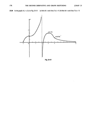
![Chapter 24
More Maximum and Minimum Problems
Until now we have been able to find the absolute maxima and minima of differentiable functions
only on closed intervals (see Section 14.2).The following result often enables us to handle cases where
the function is defined on a half-open interval, open interval, infinite interval, or the set of all real
numbers. Remember that, in general, there is no guarantee that a function has an absolute maximum or
an absolute minimum on such domains.
Theorem 24.1: Letfbe a continuous function on an interval 9,
with a single relative extremum within
9.
Then this relative extremum is also an absolute extremum on 9.
Intuitive Argument: Refer to Fig. 24-1. Suppose that f has a relative maximum at c and no other
relative extremum inside 3.Take any other number d in 9.
The curve moves down-
ward on both sides of c. Hence, if the valuef(d) were greater thanf(c), then, at some
point U between c and d, the curve would have to change direction and start moving
upward. But thenfwould have a relative minimum at U,contradicting our assumption.
The result for a relative minimum follows by applying to -f the result just obtained
for a relative maximum.
For a rigorous proof, see Problem 24.20.
1 1 1
*
C U d
Fig. 24-1
EXAMPLES
(a) Find the salortest4 istancefrom the point P(1,O) to the parabola x = y2 [see Fig. 24-2(a)].
The distance from an arbitrary point Q(x, y) on the parabola to the point P(1,O) is, by (24,
U = J -
= d
- [y2 = x at Q]
=Jx2-2X+l+x=J-
But minimizing U is equivalent to minimizing u2 =F(x) = x2 -x + 1 on the interval CO, +co)(the value of x
is restricted by the fact that x = y2 2 0).
F(x)= 2x - 1 F”(x) = 2
or x = 3
The only critical number is the solution of
F(x) = 2x - 1 = 0
Now F”(3)= 2 > 0. So by the second-derivative test, the function F has a relative minimum at x = 3. Theorem
24.1 implies that this is an absolute minimum. When x = 3,
y 2 = x = - 1 and y = + - = 1 .4 f-
4
2
-$ +JzJz= 2
Thus, the points on the parabola closest to (1,O) are (4, &2) and (4, - 4 / 2 ) .
179](https://image.slidesharecdn.com/problemscalculus-221128025033-038ef06f/85/problems-calculus-pdf-192-320.jpg)
![180 MORE MAXIMUM AND MINIMUM PROBLEMS [CHAP. 24
(b) An open box (that is, a box without a top) is to be constructed with a square base [see Fig. 24-2(b)] and is
required to have a volume of 48 cubic inches. The bottom of the box costs 3 cents per square inch, whereas the
sides cost 2 cents per square inch. Find the dimensions that will minimize the cost of the box.
Let x be the side of the square bottom, and let h be the height. Then the cost of the bottom is 3x2and the
cost of each of the four sides is 2xh, giving a total cost of
C = 3x2+4(2xh) = 3x2 +8xh
The volume is V = 48 = x2h.Hence, h = 48/x2and
384
c = 3x2 +fix@= 3x2 +-
X = 3x2 + 3fj4x-l
which is to be minimized on (0, +00). Now
and so the critical numbers are the solutions of
384
6~ ---
x2 - O
384
6~ = -
X2
x3 = 64
x = 4
Now
768
dZC
dx2 x3
- 6 - ( - 2 ) 3 8 4 ~ - ~
= 6 +-> 0
--
for all positive x; in particular, for x = 4. By the second-derivative test, C has a relative minimum at x = 4.
But since 4 is the only positive critical number and C is continuous on (0, +oo),Theorem 24.1 tells us that C
has an absolute minimum at x = 4. When x = 4,
48 48
x2 16
h = - = - = 3
So, the side of the base should be 4 inches and the height 3 inches.
tY
Fig. 24-2](https://image.slidesharecdn.com/problemscalculus-221128025033-038ef06f/85/problems-calculus-pdf-193-320.jpg)
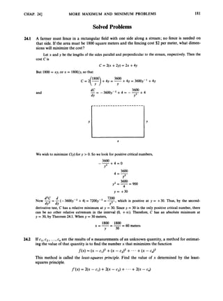
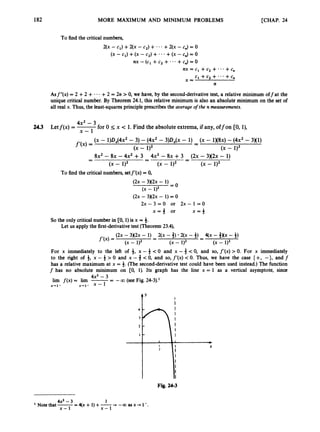
![CHAP. 241
24.4
245
24.6
24.7
24.8
24.9
24.10
24.11
24.12
MORE MAXIMUM AND MINIMUM PROBLEMS
Supplementary Problems
183
A rectangular field is to be fenced in so that the resulting area is 100 square meters. Find the dimensions of
that field (if any) for which the perimeter is: (a) a maximum; (b)a minimum.
Find the point(s)on the parabola 2x = y2 closest to the point (1,O).
Find the point(s)on the hyperbola x2 - y2 = 2 closest to the point (0, 1).
A closed box with a square base is to contain 252 cubic feet. The bottom costs $5 per square foot, the top
costs $2 per square foot, and the sides cost $3 per square foot. Find the dimensions
cost.
that will minimize the
x2 + 4
x - 2
Find the absolute maxima and minima (if any) of f(x) = -
on the interval CO,2).
A printed page must contain 60 square centimeters of printed material. There are to be margins of
5 centimeters on either side, and margins of 3 centimeters each on the top and the bottom. How long
should the printed lines be in order to minimize the amount of paper used?
A farmer wishes to fence in a rectangular field of loo00 square feet. The north-south fences will cost $1.50
per foot, whereas the east-west fences will cost $6.00 per foot. Find the dimensions of the field that will
minimize the cost.
1
Sketch the graph of y = -
1 +x2'
Find the point on the graph where the tangent line has the greatest slope.
Find the dimensions of the closed cylindrical can [see Fig. 24-4(a)] that will have a capacity of k
volume units and used the minimum amount of material. Find the ratio of the height h to the radius r
of the top and bottom. (The volume is I/ =-nr2h,and the lateral surfacearea is S = 2nrh.)
If the bottom and the top of the can have to be cut from square pieces of metal and the rest of these
squares is wasted [see Fig. 24-4(b)], find the dimensions that will minimize the amount of material
used, and find the ratio of the height to the radius.](https://image.slidesharecdn.com/problemscalculus-221128025033-038ef06f/85/problems-calculus-pdf-196-320.jpg)
![184 MORE MAXIMUM AND MINIMUM PROBLEMS [CHAP. 24
t Y
Fig. 24-5 Fig. 24-6
24.13
24.14
24.15
24.16
24.17
24.18
24.19
24.20
24.21
24.22
A thin-walled cone-shaped cup is to hold 36n cubic inches of water when full. What dimensions will mini-
mize the amount of material needed for the cup? (The volume is V = *m2h and the surface area is A = nrs;
see Fig. 24-5.)
X
(a) Find the absolute extrema on CO, +CO) (if they exist)of f ( x )= (b) Sketch the graph off:
(x2 + 1)3/2*
A rectangular bin, open at the top, is required to contain a volume of 128 cubic meters. If the bottom is to
be a square, at a cost of $2 per square meter, whereas the sides cost $0.50 per square meter, what dimen-
sions will minimize the cost?
The selling price P of an item is 100- 0.02~
dollars, where x is the number of items produced per day. If
the cost C of producing and selling x items is 4Ox + 15OOO dollars per day, how many items should be
produced and sold every day in order to maximize the profit?
Consider all lines through the point (1,3) and intersecting the positive x-axis at A(x, 0) and the positive
y-axis at B(0,y) (see Fig. 24-6).
Find the line that makes the area of ABOA a minimum.
1 k
2 x
Conisder the functionf ( x )= - x2 +-.(a) For what value of k willf have a relative minimum at x = -2?
(b) For the value of k found in part (a), sketch the graph of 1: (c) For what value(s) of k will f have an
absolute minimum?
Find the point@)on the graph of 3x2 + lOxy + 3y2= 9 closest to the origin. [Hint: Minimize x2 +y2,
making use of implicit differentiation.]
Fill in the gaps in the followingproof of Theorem 24.1. Assume thatfis continuous on an interval 9.
Letf
have a relative maximum at c in 9,
but no other relative extremum in 9.
We must show that f has an
absolute maximum on 9 at c. Assume, to the contrary, that d # c is a point in 9 withf(c) <f(d). On the
closed interval 9 with endpoints c and d,f has an absolute minimum at some point U. Sincef has a relative
maximum at c, U is different from c and, therefore,f(u) <f(c). Hence, U # d. So, U is in the interior of 9,
whencefhas a relatioe minimum at U # c.
Prove the following theorem, similar to Theorem 24.1: If the graph offis concave upward (downward)
over an interval 9,
then any relative minimum (maximum) offin 9is an absolute minimum (maximum)on
9.
[Hint: Consider the relationship of the graph offto the tangent line at the relative extremum.)
Find the absolute extrema (if any) off(x) = x2I5- 3x7/’ on (- 1, 1
3
.](https://image.slidesharecdn.com/problemscalculus-221128025033-038ef06f/85/problems-calculus-pdf-197-320.jpg)
![Chapter 25
Angle Measure
25.1 ARC LENGTH AND RADIAN MEASURE
Figure 25-l(a) illustrates the traditional system of angle measure. A complete rotation is divided
into 360 equal parts, and the measure assigned to each part is called a degree. In modern mathematics
and science, it is useful to define a different unit of angle measure.
Definition: Consider a circle with a radius of one unit [see Fig. 25-l(b)]. Let the center be C, and let
CA and CB be two radii for which the intercepted arc A
% of the circle has length 1. Then
the central angle ACB is taken to be the unit of measure, one radian.
Let X be the number of degrees in 3;ACB of radian measure 1. Then the ratio of X to 360" (a
complete rotation) is the same as the ratio of A
% to the entire circumference,211. Since A
% = 1,
360 180
or X = - = -
x 1
---
360 - 2
1
1 2
1
1 It
(25.1)
180
Thus, 1 radian = -degrees
11
If we approximate 11 as 3.14, then 1 radian is about 57.3 degrees. If we multiply (25.1) by n/180, we
obtain
11
1 degree = -radians (25.2)
180
EXAMPLE Let us find the radian measures of some "common" angles given in degrees. Clearly, the null angle is 0
in either measure. For an angle of 30", (25.2)gives
30"= 30(& radians) = radians
for an angle of 45",
45" = 45(& radians) = 4
K radians
185](https://image.slidesharecdn.com/problemscalculus-221128025033-038ef06f/85/problems-calculus-pdf-198-320.jpg)
![CHAP. 251 ANGLE MEASURE 189
(b) 390" = 360" +30" = (271 radians) +( 4 6 radians) [see Fig. 25-6(b)]. The reduced angle is 4 6 radians
(or 30").
(c) A clockwise rotation of 4 2 radians (90")
is equivalent to a counterclockwise rotation of 271 - n/2
= 3n/2 radians [see Fig. 25-6(c)].Thus, the reduced angle is 3n/2 radians.
(d) Adding a suitable multiple of 2
7
1 to the given angle, we have -3a +4
7
1 = + A radians; that is,
a clockwise rotation of 371 radians is equivalent to a counterclockwise rotation of R radians [see
Fig. 25-6(d)].The reduced angle is II radians.
SupplementaryProblems
$
25.6 Convert the followingdegree measuresof angles into radian measures: (a)36"; (b) 15";(c)2";(d)(90/n)O;
(e) 144".
25.7 Convert the following radian measuresof angles into degreemeasures: (a)2 radians; (b)4 5 radians;
(c) 7z/12 radians; (6)571/4 radians; (e)7n/6 radians.
25.8 If a bug moves a distance of 371 centimeters along a circular arc and if this arc subtends a central angle of
45", what is the radius of the circle?
25.9 In each of the following cases, from the information about two of the quantities s (intercepted arc), r
(radius),and 8 (central angle),find the third quantity. (If only a number is given for 8, assume that it is the
number of radians.)(a)r = 10, 8 = 71/5;(b)8 = 60°, s = 11/21; (c)r = 1, s = w/4; (d) r = 2, s = 3 ; (e)r = 3,
e = 900;(f)
e = 1800, = 6.283 18;(g) t = 10, e = 1200.
25.10 If a central angle of a circle of radius r measures 8 radians, find the area A of the sector of the circle
determined by the central angle (see Fig. 25-7). [Hint:
The area of the entire circle is 71r2.]
Fig. 25-7
25.11 Draw pictures of the rotations determininganglesthat measure: (a)405";(b) 11n/4radians;
(c)7n/2 radians; (d)-60"; (e)-71/6 radians; (f) -5a/2 radians.
25.12 Reduce each angle in Problem 25.11to the range of 0 to 271 radians.](https://image.slidesharecdn.com/problemscalculus-221128025033-038ef06f/85/problems-calculus-pdf-202-320.jpg)
![Chapter 26
/ * - '
/'
/
/
Sine and Cosine Functions
-
26.1 GENERAL DEFINITION
1 0
The fundamental trigonometric functions, the sine and the cosine, will play an important role in
calculus. These functionswill now be defined for all real numbers.
Definition: Place an arrow 03 of unit length so that its initial point 0 is the origin of a coordinate
system and its endpoint A is the point (1, 0) of the x-axis (see Fig. 26-1). For any given
number 8, rotate about the point 0 through an angle with radian measure 8. Let 0
be the final position of the arrow after the rotation. Then: (i) the x-coordinate of B is
defined to be the cosine of 8, denoted by cos 8; (ii) the y-coordinate of B is defined to be
the sine of 8, denoted by sin 8. Thus, B = (cos 8, sin 8).
-
1 X
f'
, I
Fig. 26-1
EXAMPLES
(a) Let 8 = n/2.If we rotate OA x/2 radians in the counterclockwise direction, the final position B is (0, 1) [see
Fig. 26-2(u)].Hence,
11 x
sin - = 1
2
cos-=o
2
(b) Let 8 = x. If we rotate FA through K radians in the counterclockwisedirection, the final position B is (- 1,O)
[see Fig. 26-2(b)].So,
cos Ic = -1 sin 7c = 0
f Y
(6)
Fig. 26-2
190](https://image.slidesharecdn.com/problemscalculus-221128025033-038ef06f/85/problems-calculus-pdf-203-320.jpg)
![CHAP. 261 SINE AND COSINE FUNCTIONS 191
(c) Let 6 = 3z/2. Then the final position B, after a rotation through 3z/2 radians in the counterclockwise direc-
tion, is (0, -1)[see Fig. 26-2(c)]. Hence,
3n 3n
2 2
cos -= 0 sin -= -1
(6) Let 8 = 0. If is rotated through 0 radians, the finalposition is still (1,O). Therefore,
cos 0 = 1 sin 0 = 0
(e) Let 8 be an acute angle (0 < 6 < n/2)of right triangle DEF, and let AOBG be a similar triangle with hypot-
enuse 1 (see Fig. 26-3). By proportionality, = b/c and = a/c. So, by definition, cos 6 = a/c,
sin 8 = b/c.This agreeswith the traditional definitions:
adjacent side
hypotenuse
cos e =
E
opposite
side,b
opposite side
hypotenuse
sin 8 =
Y
B(COS
8, sin 8)
D adjacent F O E G X
Fig. 26-3
side, a C
Consequently,we can appropriate the values of the functions for 8 = n/6, 44, n/3 from high-school trigonom-
etry. The results are collectedin Table 26-1, which ought to be memorized.
Table 26-1
6](https://image.slidesharecdn.com/problemscalculus-221128025033-038ef06f/85/problems-calculus-pdf-204-320.jpg)

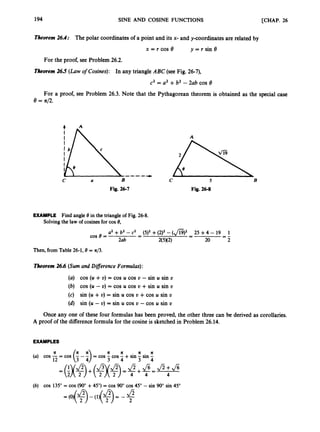
![CHAP. 26) SINE AND COSINE FUNCTIONS 195
In 7 1 7 1 7 1 7 1
12 2 12 2 12
(c) sin -= sin (2 +5)= sin 5cos 5+cos - sin -
= (l)( Jz+& )+(O)(sin :
) [by example (a)]
SubstitutingU = a/2 and U = 8in the differenceformulasof Theorem 26.6yields
a 1c
cos (i- 8 ) = cos 5cos 8 +sin - sin 8 = 0 cos 8 + 1 sin 8 = sin 8
sin (F- 8) = sin 5cos 8 - cos - sin 8 = 1 cos 8 - 0 sin 8 = cos 8
2
2
a II
Thus we have:
Theorem26.7: cos (i- 8) = sin 8 and sin (;,- 8) = cos 8; that is, the sine of an angle is the cosine
of its complement.
We also have the useful double-angleformulas :
Theorem26.8: cos 28 = cos28 -sin28 = 2 cos28 - 1 = 1 - 2 sin28 and sin 28 = 2 sin 8 cos 8.
For cos 28, note that:
(i) cos 28 = cos (8 +8)= cos 8 cos 8 - sin 8 sin 8
(ii)
[by Theorem 26.6(a)]
p y Theorem 26.11
[by (ii) and Theorem 26.11
= cos2 8 - sin28
= cos28 - (1 - cos28)
= 2 cos2 8 - 1
= (1.- sin28) - sin28
= 1 - 2 sin28
For sin 28,
sin 28 = sin (8 +8) = sin 8 cos 8 +cos 8 sin 8 [by Theorem 26.6(c)]
= 2 sin 8 cos 8
From Theorem 26.8,we deduce:
Theorem26.9 (Half-AngleFormulas):
8 1 +cos 8
2
8 1 -cos 8
2
2
2
(a) cos2- =
(b) sin2- =
In fact,replace 8 by 812 in Theorem 26.8:
8 1 +COS e
2 '
2
8 8 1 -cos 8
2' 2 2 .
(a) cos 8 = cos - 1. so, cos2 - =
(6) COS 8 = COS - So, sin2- =
EXAMPLES
(a) sin 120"= sin (2 x 60")
= 2 sin 60"cos 60"](https://image.slidesharecdn.com/problemscalculus-221128025033-038ef06f/85/problems-calculus-pdf-208-320.jpg)
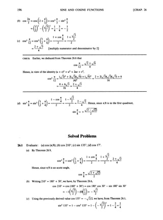
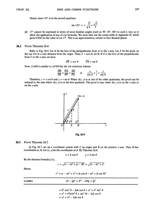
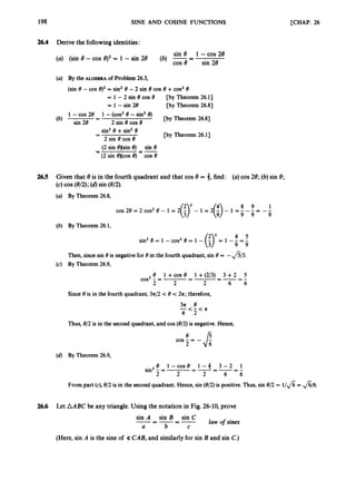
![CHAP. 261 SINE AND COSINE FUNCTIONS 199
Let D be the foot of the perpendicularfrom A to side BC. Let h = AD. Then,
-
or h = c sin B
AD h
sin B === -
AB c
and so
1 1 1
2 2 2
area of AABC = -(base x height) = - ah = - ac sin B
(Check that this is also correct when 9:B is obtuse.) Similarly,
1
2
area =- ab sin C
1
area = - bc sin A
2
Hence,
1 1 1
- ac sin B = - bc sin A = - ab sin C
2 2 2
and division by 4abc gives the law of sines.
A
B D a C
Fig. 26-10
Supplementary Problems
26.7 Evaluate: (a) sin (4n/3); (b) cos (lln/6); (c) sin 240"; (6)cos 315";(e) sin 75"; (f)sin 15";(9) sin (11n/12);
(h) cos 71";(i) sin 12".
26.8 If 8 is acute and cos 8 = 4, evaluate: (a) sin 8;(b) sin 28; (c)cos 28;(d) cos (8/2);(e) sin (8/2).
26.9 If 8 is in the third quadrant and sin 8 = -3,evaluate: (a) cos 8;(b) sin 28; (c)cos 28;(d) cos (8/2);
(e)sin (8/2).
26.10 In AABC, AB = 5, AC = 7, and = 6. Find cos B.
26.11 In Fig. 26-11, D is a point on side BC of AABC such that AB = 2, AD = 5,
[Hint:
U
s
e the law of cosines twice.]
= 4, and = 3. Find x.
26.12 Prove the followingidentities:
1 +cos 28 cos e
--
(a) cos258 = (1 - sin 5e)(i +sin 58) (b) -
sin 28 sin 8
(c) (sin 8 +cos 8)2= 1 +sin 28 (6) cos4 8 - sin48 = cos2 8 - sin28](https://image.slidesharecdn.com/problemscalculus-221128025033-038ef06f/85/problems-calculus-pdf-212-320.jpg)
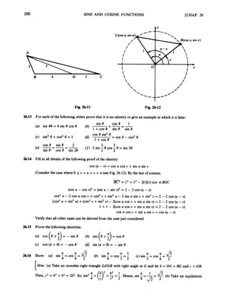
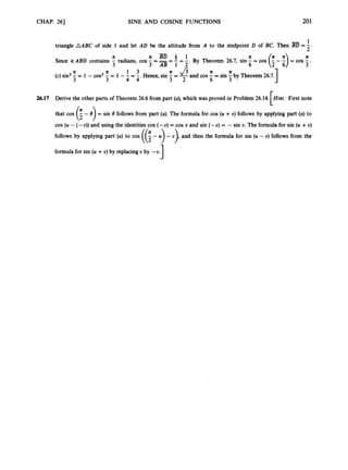
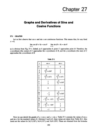
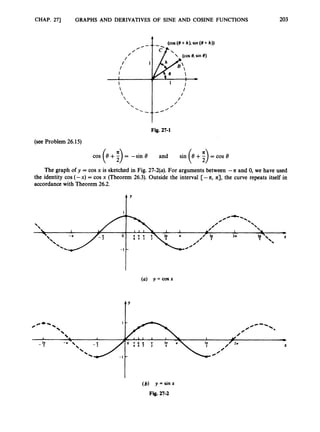
![204 GRAPHS AND DERIVATIVES OF SINE AND COSINE FUNCTIONS [CHAP. 27
The graph of y = sin x [see Fig. 27-2(6)] is obtained in the same way. Notice that this graph is the
result of moving the graph of y = cos x to the right by 4 2 units. This can be verified by observingthat
cos (x -;
) = sin x
The graphs of y = cos x and y = sin x have the shape of repeated waves, with each complete wave
extending over an interval of length 2n (the period). The length and height of the waves can be changed
by multiplying the argument and the functional value, respectively, by constants.
EXAMPLES
(a) y = cos 3x. The graph of this function is sketchedin Fig. 27-3. Because
cos 3 x +- = cos (3x +2n) = cos 3x
( 3
the function is of period p = 2n/3. Hence, the length of each wave is 2n/3. The number of waves over an
interval of length 2n (corresponding to one complete revolution of the ray determining angle x) is 3. This
number is called thefrequencyfof cos 3x. In genera),
pf= (length of each wave) x (number of waves in an interval of length 2n) = 2%
and so
2R
P
f = -
For an arbitrary constant b > 0, the functioncos bx (or sin bx) has frequencyb and period 2n/b.
Fig. 27-3
(b) y = 2 sin x. The graph of this function (see Fig. 27-4) is obtained from the graph of y = sin x (see Fig. 27-2) by
multiplying each ordinate by 2. The period (wavelength)and the frequencyof the function 2 sin x are the same
as those of the function sin x: p = 27c,f= 1. But the amplitude, the maximum height of each wave, of 2 sin x
is 2, or twice the amplitude of sin x.
NOTE The total oscillation of a sine or cosine function, which is the vertical distance from crest to trough, is
twice the amplitude.](https://image.slidesharecdn.com/problemscalculus-221128025033-038ef06f/85/problems-calculus-pdf-217-320.jpg)
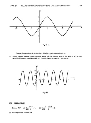
![206 GRAPHS AND DERIVATIVES OF SINE AND COSINE FUNCTIONS [CHAP. 27
1 -cos e 1 +cos e 1 - cos2 e
= lim
i - m s e
(b) lim = lim
e-ro 6 0-0 8 1+cos 0 e+o e(l +cos 0)
sin 8 sin 8
Xlim-0
sin2 8
= lim
= lim - lim
Theorem 2
7
.
2
; D,(sin x) = cos x and D,(cos x) = -sin x.
0-0 e(l +cos 8) e+o 0 1 +cos 8
0 4 0 8 e-ro 1 +cos8 1 + 1
= I * - = O O
sin 8 sin 8
For the proof, see Problem 27.5.
EXAMPLES
(a) Find DJsin 2x). The function sin 2x is a composite function. If f ( x )= 2x and g(x) = sin x, then
sin 2x = g(f(x)).The chain rule (15.2)gives
or
(b) Find Dx(c0s4x). The function cos4x is a composite function. Iff(x) = cos x and g(x) = x4, then
cos4 x = (COS
x ) ~
= g(f(x))
Therefore, D,(c0s4 x) = D,((cos x)~)
= *cos x ) ~D,(cos x)
= qcos x)’ (-sin x)
= -4 cos3 x sin x
[by the power chain rule]
Solved Problems
27.1 Find the period, frequency,and amplitude of:
X 1
2 2
(a) 4 sin - (b) -cos 3x
and sketch their graphs.
2n 2n
(a) For 4 sin i x A sin bx, the frequency isf= 6 = 4, the period is p = -= -= 4n, and the amplitude
f 3
is A = 4. The graph is sketched in Fig. 27-qa).
2n 2n
(b) For 4 cos 3x E A cos bx, the frequencyf is b = 3, the period is p = -= - and the amplitude is
b 3 ’
A = 4. The graph is sketched in Fig. 27-6(b).
Fig. 27-6](https://image.slidesharecdn.com/problemscalculus-221128025033-038ef06f/85/problems-calculus-pdf-219-320.jpg)
![CHAP. 273 GRAPHS AND DERIVATIVES OF SINE AND COSINE FUNCTIONS 207
27.2 Find all solutions of the equations:
1
(a) cos x = 0 (b) sin x = -
2
(a) For -a 5 x < a, inspection of Fig 27-2(a)shows that the only solutions of cos x = 0 are
a
x = -- and x=lf
2 2
Since 211 is the period of cos x, the solutions of cos x = 0 are obtained by adding arbitrary integral
multiples of 271 to -n/2 and a/2,
a ‘ a a a
2 2 2 2
- - +2zn = - (4n - 1) and - +2an = - (4n - 1)
Together, 4n - 1 and 4n + 1 range over all odd integers, and so the solutions of cos x = 0 are all odd
multiples of 4 2 ,
n
x = (2k + 1)5 [k = 0, f1, f 2 , ...I
(b) Figure 27-2(b)shows that, for -a/2 5 x < 37c/2, the only solutions are x = a/6 and x = 5a/6. Hence,
all the solutions are
a 5n
-+2an and -++an
6 6
wheren=O,+l,f2 ,....
27.3 Find the derivatives of:
X X
(a) 3 sin Sx (b) 4 cos - (c) sin’ x (6) cos3-
2 2
(a) D,(3 sin 5x) = 3D,(sin 5x)
= COS 5x)DX(5x)
= COS 5 ~ x 5 )
= 15 COS 5x
[by the chain rule and Theorem 27.2)
(b) Dx(4 cos ;
) = 4D,(cos ;
)
= 4( -sin ;)Dx( ;
) [by the chain rule and Theorem 27.2)
= -(sin ;)(:) = -2 sin -
X
2
(c) DJsin’ x) = DJsin x)’)
= (2 sin x)D,(sin x)
= 2 sin x cos x
= sin 2x
b y the power chain rule]
[by Theorem 27.23
[by Theorem 26.83
= 3( COS COS ;
) [by the power chain rule]
= (3 cos’ ;)( - (sin i)D,(;))
[by the chain rule and Theorem 27.2)
3 x x
2 2 2
= cos2 :)( - sin :
) = -- cos2 - sin -](https://image.slidesharecdn.com/problemscalculus-221128025033-038ef06f/85/problems-calculus-pdf-220-320.jpg)
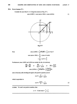
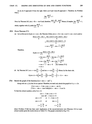
![210 GRAPHS AND DERIVATIVES OF SINE AND COSINE FUNCTIONS [CHAP. 27
x f(x>
1
6 4
0
2
1
5n
6 4
3n
- 2
2
-
n
-
n
-
-
-
- 2
-'I
f"(x)
rel. max.
3
2
1 rel. min.
1
2
3 re1 min.
--
rel. max.
--
Fig. 27-8
Table 27-2
27.7 Find the absolute extrema of the functionf(x) = 2 sin x -cos 2x on the closed interval [0, lt].
For this simple function it is unnecessary to resort to the tabular method of Section 14.2. It suffices to
observe that the sine and cosine functions have maximum absolute value 1. Thus, if there is an argument x
in [0, n] such that
f(x) = 2(+1) -(-1) = 3
that argument must represent an absolute maximum (on any interval whatever). Clearly, there is one and
only one such argument, x = n/2.
On the other hand, since sin x 2 0 on [0, n], the arguments x = 0 and x = n minimize sin x and, at the
same time, maximize cos 2x. Hence,
f(0) =f(n)= 2(0) -(+I) = -1
is the absolute minimum value on [0, n].
SupplementaryProblems
27.8 Find the period,frequency, and amplitude of each function, and sketch its graph.
4x 1
2
3
(6) - sin 3x
(a) cos -](https://image.slidesharecdn.com/problemscalculus-221128025033-038ef06f/85/problems-calculus-pdf-223-320.jpg)
![CHAP. 271 GRAPHS AND DERIVATIVES OF SINE AND COSINE FUNCTIONS 211
27.9 Find the period, frequency,and amplitude of:
X 5x
3 2
(a) 2 sin - (b) -cos 2x (c) 5 sin - (d) cos (-4x)
[Hint: In part (d), the function is even.]
27.10 Find all solutions of the followingequations:
(a) sin x = 0 (b) cos x = 1 (c) sin x = 1 (d) cos x = -1
(e) sin x = -1 (j)cos x = -
1 (9) sin x = Jz (h) cos x = -
J5
2 2 2
[Hint: By Theorem 26.1, only two of parts (a),(b), and (d)need be solved.]
27.11 Find the derivativesof the followingfunctions:
(a) 4 sin3 x (b) sin x +2 cos x (c) x sin x (d) x2 cos 2x
sin x 1- cos x
(4 x ( f ) x2 (9) 5 sin 3x cos x (h) cos2 2x
(i) cos (2x2- 3) 0
1 sin3 (5x +4) (k) JZZG (0 sin3 (sin2x)
27.12 Calculate the followinglimits:
sin x
(a) lirn -
x+o 3x
cos x - 1 sin 2x x + l
(b) lirn (c) lirn - (d) lirn -
x+o 2x x-ro sin 3x x-ro cos x
sin 4x
(e) lim -
x-ro 5x
cos 3x
(h) lirn -
x-rn/2 cosx
sin3 x sin x2
(f) lim -
im x cos -
0 1'
(9) lim x
x-ro 4x3 x+o
2 -x cos x
(I) lim
1 (k) sin2(x - 4)
x-ro X2 x-ro X2 x+4 (x -412 x-r+Q)x2 +x + 1
x sin 4x -sin2x
(i) lirn
27.13 Sketch the graphs of the followingfunctions:
(a) f(x) = sin2x (b) g(x) = sin x +cos x (c) f(x) = 3 sin x -sin3 x
(d) h(x)= cos x -cos2x (e) g(x) = Isin x I
(9) f(x) = sin (x - 1)
(h)
(f)f ( x )= sin x +x
Check your answers to parts (a)-(g) on a graphing calculator.
27.14 Find the absolute extrema of each function on the given interval:
sin x +x on [0, 2
1
1
1
2 sin x +sin 2x on CO, 2
7
1
1
3 sin x -4 cos x on CO, 2
1
1
1
(b) sin x -cos x on CO, n]
(e) lcos x - on CO, 2nl
(c) cos2 x +sin x on [0, A]
1
(f)- x - sin x on CO, 2nl
2
Show that f(x) = A cos x +B sin x has pdriod 2n and amplitude ,
/
-
. Hint: Clearly,
[
B
S 1. Hence, there exists cp such that
A
IJAand IJml
f(x +2n) =f(x). Note that
sin cp = Jm
and cos cp =
1
.Show thatf(x) = ,/mi
sin (x +cp).
A B
Jm
Find the amplitude and period of: (i)3 cos x -4 sin x; (ii)5 sin 2x + 12cos 2x;
(iii)2 cos x +,/5 sin x.](https://image.slidesharecdn.com/problemscalculus-221128025033-038ef06f/85/problems-calculus-pdf-224-320.jpg)
![212
2
7
.
1
6
27.17
27.18
27.19
27.2~
2
7
.
2
1
27.22
27.23
27.24
27.25
27.26
GRAPHS AND DERIVATIVES OF SINE AND COSINE FUNCTIONS [CHAP. 27
COS (
: +h) - 1
2
h
(b) lim
h b+O
Evaluate: (a) lim
[Hint: Recall the definitionof the derivative.]
h-0
For what value of A does 2 sin Ax have period 2?
Find an equation of the tangent line to the graph of y = sin2x at the point where x = n/3.
Find an equation of the normal line to the curvey = 1 +cos x at the point (n/3,3/2).
Find the smallest positive integer n such that D:(cos x) = cos x.
Letj(x) = sin x +sin Ix I.(a)Sketch the graph off: (b) Isfcontinuous at O? (c) Isfdifferentiable at x = O?
Find the slope of the tangent line to the graph of:
(a) y = x +cos (xy) at (0, 1); (b) sin (xy) = y at (n/2, 1).
[Hint:Use implicit differentiation.]
Use implicit differentiationto find y':
cos y = x (b) sin (xy) = y2
A ladder 26 feet long is leaning against a vertical wall (see Fig. 27-9). If the bottom of the ladder A is
slippingaway from the base of the wall at the rate of 3 feet per second,how fast is the angle 8 between
the ladder and the ground changingwhen the bottom of the ladder is 10feet from the base of the wall?
An airplane is ascending at a speed of 400 kilometers per hour along a line making an angle of 60"
with the ground. How fast is the altitude of the plane changing?
A man at a point P on the shore of a circular lake of radius 1 mile (see Fig. 27-10) wants to reach the
point Q on the shore diametrically opposite P.He can row 1.5 miles per hour and walk 3 miles per
hour. At what angle 8 (0 5 8 5 4 2 ) to the diameter PQ should he row in order to minimize the time
required to reach Q? (When 8 = 0, he rows all the way;when 8 = n/2,he walks all the way.)
Rework part (a) if, instead of rowing, the man can paddle a canoe at 4 miles per hour.
Fig. 27-9 Fig. 27-10
Find the absoluteextrema off@) = x - sin x on CO, 421.
From part (a),infer that sin x < x holds for all positive x.
sin x
Verifyon a graphing calculator that cos x 5 -5 1for x # 0 and -(n/2) I x 5 (n/2).
X](https://image.slidesharecdn.com/problemscalculus-221128025033-038ef06f/85/problems-calculus-pdf-225-320.jpg)
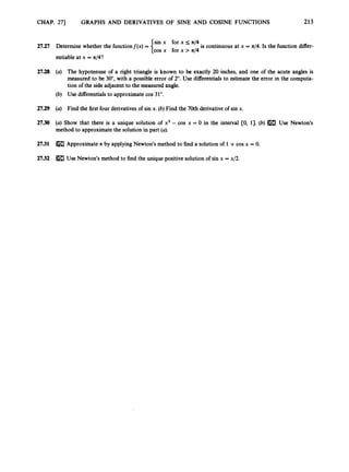
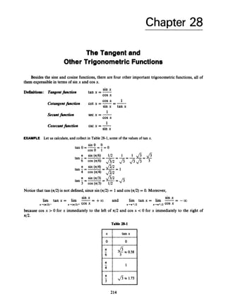
![216 THE TANGENT AND OTHER TRIGONOMETRIC FUNCTIONS [CHAP. 28
Tkorem 283 (Identities): tan’ x + 1 = sec’ x and cot’ x + 1= csc’ x.
Proof: Divide sin2x +cos2x = 1 by cos’ x or sin2x.
Traditional Definitions
As was the case with sin 8 and cos 8, the supplementary trigonometric functions were originally
defined only for an acute angle of a right triangle. Referringto Fig. 26-3, we have
opposite side
adjacent side
adjacent side
opposite side
hypotenuse
adjacent side
hypotenuse
opposite side
tan 8 =
cot 8 =
sec 8 =
csc e =
SolvedProblems
28.1 Prove Theorem 28.2.
DAtan x) = D,(-)sin x
cos x
(cos x)D,(sin x) -(sin x)D,(cos x)
-
- [by the quotient rule]
(cos x)2
(cos xxcos x) -(sin x)(-sin x)
cos2x
-
- [by Theorem 27.21
cos2x +sin’ x 1
- -
cos2x cos’ x
[by Theorem 26.11
= sec2x
-1
(tan x ) ~
D,(cot x) = D,((tan x)- l) = -
DAtan x) [by the power chain rule]
-1 1 -1
-1 sin x
=
-
-
=
(tan x ) ~
(cos x ) ~
(sin x)’
= -csc2 x
(tan x cos x)’
I
=- [tan x =
Differentiatingthe first identity of Theorem 28.3,
2(tan x)(sec2 x) = 2(sec x)D,(sec x)
and dividing through by 2(sec x), which is never zero, gives
D,(sec x) = tan x sec x
Similarly,differentiationof the second identity of Theorem 28.3 gives
D,(csc x) = -cot x csc x](https://image.slidesharecdn.com/problemscalculus-221128025033-038ef06f/85/problems-calculus-pdf-229-320.jpg)
![CHAP. 281 THE TANGENT AND OTHER TRIGONOMETRIC FUNCTIONS
I
I
1 I 1
-3 -? -? -:()
217
I
I
1 1 1
I 5 & ; +
4 1 x
28.2
2
8
.
3
28.4
Draw the graph of csc x.
only find the graph for 0 c x < a. Now
Because csc x = l/(sin x), it is, along with sin x, periodic, of period 2n, and odd. Therefore, we need
- 1
n 1 1
2 sin (42) 1
csc - = -
= - -
As x decreases from n/2 toward 0, sin x decreases from 1 toward 0. Therefore, csc x increases from 1 to
+CO. Likewise, as x increases from z/2 toward n,sin x decreases from 1toward 0, and csc x increases from
1 to +a.
In fact, since sin ((a/2)+U) = sin ((42) - U), the graph will be symmetric about the line x = n/2
(see Fig. 28-2).
Fig. 28-2
tan U - tan U
1 +tan u tan U ’
Prove the identity tan (U - U) =
sin (U - U) sin U cos U -cos U sin U
cos (U - U) - cos U cos U +sin U sin U
tan (U - U) = - [by Theorem 26.63
sin U sin U
---
cos U cos U
-
- .[divide numerator and denominator by cos U cos U]
sin U sin U
1+--
tan U - tan U
1 +tan U tan U
cos U cos U
-
-
Calculate: (a)0,(3 tan2x); (b)D,(sec x tan x).
(a) D,(3 tan’ x) = 3D,(tan2 x) = 3(2 tan x)D,(tan x) [by the power chain rule]
= 6 tan x sec’ x
(b) D,(sec x tan x) = (sec x)D,(tan x) +(tan x)DJsec x) [by the product rule]
[by Theorem 28.21
[by Theorem 28.31
= (sec x)(sec2x) +(tan x)(tan x sec x)
= (sec x)(seczx +tan’ x)
= (sec x)(sec2x +tan’ x)
= (sec x)(tan2x + 1+tan’ x)
= (sec x)(2 tan’ x + 1)](https://image.slidesharecdn.com/problemscalculus-221128025033-038ef06f/85/problems-calculus-pdf-230-320.jpg)
![218 THE TANGENT AND OTHER TRIGONOMETRIC FUNCTIONS [CHAP. 28
28.5 A lighthouse H, 1mile from a straight shore, has a beam that rotates counterclockwise(as seen
from above) at the rate of six revolutions per minute. How fast is point P, where the beam of
light hits the shore, moving?
Let A be the pont on shore opposite H, and let x be the distance AP (see Fig. 28-3). We must find
dx/dt. Let 0 be the measure of 3:PHA. Since the beam makes six revolutions (of 2n radians) per minute,
--
- 12n radians per minute
d8
dt
Now
Hence,
I
opposite side
adjacent side
dx dt?
- D,(tan 0) = &(tan 0) -
dt dt
- - [by the chain rule]
1
hypotenuse
adjacent side
= (sec2 0x127c) = ( ~ ~ ~ i ) 2 ( 1 2 n )
[since sec e =
= 12n(x2+ 1)
For instance, when P is 1 mile from A, the light is moving along the shore at 24n miles per minute (about
4522 miles per hour).
28.6 The angle o
f inclination of a nonvertical line 2' is defined to be the smaller counterclockwise
angle a from the positive x-axis to the line (see Fig. 28-4). Show that tan a = m,where m is the
slope of 9.
By taking a parallel line, we may always assume that 9 goes through the origin (see Fig. 28-5). 9
intersects the unit circle with center at the origin at the point P (cos a, sin a). By definition of slope,
sin a - 0 sin a
cosa-0 cosa
=--
m = - tan a
I
I
A X P
'
,
Fig. 28-3 Fig. 28-4
28.7 Find the angle at which the lines S1
: y = 2x + 1 and s2:y = -3x +5 intersect.
Let a1 and a2 be the angles of inclination of LZ1and S2(see Fig. 28-6),and let ml and m2 be the slopes
of Y1
and g2.
By Problem 28.6, tan a, = rn, = 2 and tan a2 = m2 = -3. a2 -a1 is the angle of intersec-
tion. Now
tan a2 - tan a1
1 +tan a, tan a2
m2 - m1
1 +mlm2
tan (a2- a l ) =
-
-
[by Problem 28.33
[by Problem 28.63
1
-5 -5
1+(-3x2) 1 - 6 -5
=-=-=
-3 - 2
-
-](https://image.slidesharecdn.com/problemscalculus-221128025033-038ef06f/85/problems-calculus-pdf-231-320.jpg)
![220 THE TANGENT AND OTHER TRIGONOMETRIC FUNCTIONS [CHAP. 28
28.15 A rocket is rising straight up from the ground at a rate of loo0 kilometers per hour. An observer 2
kilometers from the launchingsite is photographing the rocket (see Fig. 28-7). How fast is the angle 8of the
camera with the ground changingwhen the rocket is 1.5 kilometers above the ground?
0
’
0
’
0
’
0
0
’
Y
0
0
’
2
Fig. 28-7
/-
A/?@
2
Fig. 28-7
28.16 Find the angle of intersectionof the lines Yl: y = x - 3 and Y 2 : y = -5x +4.
28.17 Find the angle of intersection of the tangent lines to the curves xy = 1 and 9 = x3 at the common point
(1, 1).
28.18 Find the angle of intersection of the tangent lines to the curves y = cos x and y = sin 2x at the common
point (46, &2).
28.19 Find an equation of the tangent line to the curve 1 + 16x2y = tan (x -2y) at the point (n/4,0).
28.20 Find the relative maxima and minima, inflection points, and vertical asymptotes of the graphs of the follow-
ing functions,on [O,a] :
(a) f ( x ) = 2x -tan x (6) f ( x )= tan x - 4x
2.8.21 Find the intervalswhere the functionf(x) = tzn x -sin x is increasing.
28.22 Use Newton’s method to approximatesolutions of the followingequations: (a)sec x = 4 on CO, a/2];
(b) tan x - x = 0 on [n,3n/2]; (c) tan x = l/x on (0,a).](https://image.slidesharecdn.com/problemscalculus-221128025033-038ef06f/85/problems-calculus-pdf-233-320.jpg)
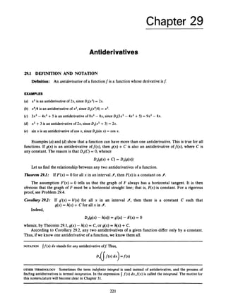
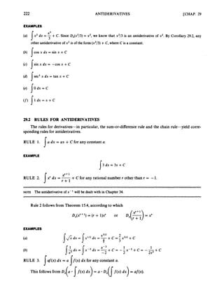
![CHAP. 291 ANTIDERIVATIVES 225
(a) Notice that DJ2x3 -x) = 6x2- 1. So, by quick formula I,
1
(2x3- ~ ) ~ ( 6 x ~
- 1) dx = - (2x3- x)' +C
I 5
(b) Observe that Dx(5x2- 1) = 1Ox. Then, by Rule 1,
J ~ G Z dx = ( 5 2 - 1 p 3 dx = -J ( 5 2 - 11113 iox dx
10
1 ( 5 2 - 1)4/3 +
10 4
p y quick formula I]
I
=Ad-+c
40
=-
3 3
40 40
= -pX2
- 11413 +c = -(
4
-
1
~+c
(For manipulations of rational powers, review Section 15.2.)
293 Use the substitution method to evaluate:
(a) Let u = &.Then,
1
du = DJ&) dx = Dx(X"2) dx = - x-1/2 dx = -
2 2> dx
d x = 2 sinudu= - ~ C O S U + C = - ~ C O S & + C
s
Hence,
(b) Let U = 3x2 - 1. Then du = 6x dx, and
x sec2(3x2 - 1) dx =-
1 1
s 6
'
I 6 6
sec2u du = - tan u + C = - tan (3x2 - 1) +C
(c) Let u = x +2. Then du = dx and x = u - 2. Hence,
Ix 2 , / z dx = I(U - 2)2& du = I(u2 -4u +4)u1I2du
= { ( u ~ / ~
- 4u3I2+4u1/') du
2 8 8 2 8 8
-
-- u7i2 -- u5i2 + - u ~ i z
7 5 3
[by du" = ur+q
+c = (x +2)7/2- (x +2)5/2+ (x +2)3/2+c
The substitution U = ,
/
=
would also work.
29.4 Prove Theorem 29.1.
Let a and b be any two numbers in 9.
By the mean-value theorem (Theorem 17.2), there is a number c
between a and b, and therefore in 9,
such that
But by hypothesis, F'(c)= 0; hence, F(b)-F(a) = 0, or F(b)= F(a).](https://image.slidesharecdn.com/problemscalculus-221128025033-038ef06f/85/problems-calculus-pdf-238-320.jpg)
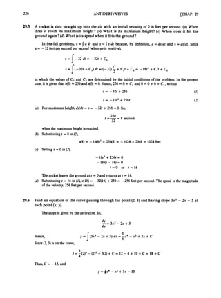
dx (c) 5 2 f i dx
(6) 1 5 P d x (4 j$dx (f) j ( x ' - 1)fidx
(0) I x ( x 4 +2)2dx
s
(9) I($-+
U) s ( 7 sec2 x - sec x tan x) dx
(m)I
' dx
(h) s"'-;+ 1 dx
(k) (csc2 x +3x2) dx
(n) !tan2 x dx
(i) I ( 3 sin x +5 cos x) dx
(0 1x ~ 3 x
dx
sec x
[Hint:
Use Theorem 28.3 in (n).)
29.8 Evaluate the followingantiderivatives by using Rule 5 or Rule 6. [In (m),a # 0.1
X
(d) Isin (3x - 1) dx (e) /sec2 5dx
(9) I ( 4 - 2t2)7t dt (h) sx2,./;'Ti dx (i) X dx
x + l
(f) l v d x
U) 1d x m , dx (k) (x* + 1)ll3x7dx
s
(m)I.,/=
dx
(p) J(3x - 5)l2x dx
(s) 1ssec2 2dx
(n) I & X
cos 3x
(4) "4 - 7t2)7tdt
(0) s,/G
x2 dx
sin (l/x) cos (l/x)
dx
3
29.9 A rocket is shot vertically upward from a tower 240 feet above the ground, with an initial velocity of 224
feet per second. (a)When will it attain its maximum height? (b) What will be its maximum height? (c)When
will it strike the ground? (d) With what speed will it hit the ground?
29.10 (Rectilinear Motion, Chapter 18) A particle moves along the x-axis with acceleration a = 2t - 3 feet per
second per second. At time t = 0, it is at the origin and moving with a speed of 4 feet per second in the
positive direction. (a) Find a formula for its velocity U in terms of t. (b) Find a formula for its position x in
terms of t. (c) When and where does the particle change direction? (d) At what times is the particle moving
toward the left?
29.11 Rework Problem 29.10 if a = t2 - 9feet per second per second.
29.12 A rocket shot straight up from ground level hits the ground 10 seconds later. (a) What was its initial
velocity? (b) How high did it go?](https://image.slidesharecdn.com/problemscalculus-221128025033-038ef06f/85/problems-calculus-pdf-240-320.jpg)
![228 ANTIDERIVATIVES [CHAP. 29
29.13 A motorist applies the brakes on a car moving at 45 miles per hour on a straight road, and the brakes cause
a constant deceleration of 22 feet per second per second. (a) In how many seconds will the car stop? (b)
How many feet will the car have traveled after the time the brakes were applied? [Hint: Put the origin at
the point where the brakes were initially applied, and let t = 0 at that time. Note that speed and deceler-
ation involvedifferent units of distance and time; changethe speed to feet per second.]
29.14 A particle moving on a straight line has acceleration a = 5 - 3t, and its velocity is 7 at time t = 2. If s(t) is
the distancefrom the origin at time t, find 42)-$1).
29.15 (a) Find the equation of a curve passing through the point (3, 2) and having slope 2x2 - 5 at point (x, y),
(b) Find the equation of a curve passing through the point (0, 1)and having slope 12x + 1 at point (x, y
)
.
29.16 A ball rolls in a straight line, with an initial velocity of 10 feet per second. Friction causes the velocity to
decrease at a constant rate of 4 feet per second per second until the ball stops. How far will the ball roll?
[Hint: U = -4 and uo = 10.1
29.17 A particle moves on the x-axis with acceleration u(t) = 2t - 2 for 0 I; t I; 3. The initial velocity uo at t = 0
is 0. (a) Find the velocity Nt). (6)When is u(t) c O? (c) When does the particle change direction?(d)Find the
displacement between t = 0 and t = 3. (Displacement is the net change in position.) (e) Find the total dis-
tance traveled from t = 0 to t = 3.
29.18 Justify the followingform of the substitutionmethod (Rule6):
If(g(x))c?’(x)
dx = 1f(4du
/
where U is replaced by g(x) after integration on the right. The “substitution” would be applied to the
left-hand side by letting U = g(x) and du = g’(x) dx. [Hint: By the chain rule,](https://image.slidesharecdn.com/problemscalculus-221128025033-038ef06f/85/problems-calculus-pdf-241-320.jpg)
![Chapter 30
The Definite Integral
30.1 SIGMA NOTATION
The Greek capital letter Z is used in mathematics to indicate repeated addition.
EXAMPLES
99
X i = 1 +2 +3 +-..+99
that is, the sum of the first 99 positive integers.
c ( 2 i - 1)= 1 + 3 + 5 + 7 + 9 + 11
that is, the sum of the first six odd positive integers.
i = 1
6
i=
1
5 5
c 3 i = 6 +9 + 12 + 15 = 3(2 +3 +4 + 5) = 3
c
i
i = 2 i = 2
j2 = l2+22 +32 + * . * + 152 = 1 +4 +9 +
15
j = 1
5
+ 225
C sinjn = sin n +sin 2n +sin 311 +sin 4n +sin 5n
j = 1
In general, given a functionfdefined on the integers,and given integers k and n 2 k,
n
f(i) = f ( k ) + f ( k + 1) + -..+f(n)
i = k
30.2 AREA UNDER A CURVE
Letfbe a function such thatf(x) 2 0 for all x in the closed interval [a, b]. Then its graph is a curve
lying on or above the x-axis (see Fig. 30-1). We have an intuitive idea of the area A of the region 9 lying
under the curve, above the x-axis, and between the vertical lines x = a and x = 6. Let us set up a
procedure for finding the value of the area A.
Select points xl, x2,...,x,- inside [a, 61 (see Fig. 30-2). Let xo = a and x, = 6,
a = xo <x1 < x2 < * ' < x,-1 <x, = b
These divide [a, b] into the n subintervals [xo, xl], [xl, x2], ..., [ x ~ - ~ ,
x,]. Let the lengths of these
subintervalsbe Alx, A2x, ...,A,,x, where
Aix E xi - x1-1
Draw vertical lines x = xi from the x-axis up to the graph, thereby dividing the region 9 into n strips. If
AiA is the area of the ith strip, then
n
A = C A i A
I=1
229](https://image.slidesharecdn.com/problemscalculus-221128025033-038ef06f/85/problems-calculus-pdf-242-320.jpg)
![230 THE DEFINITE INTEGRAL [CHAP. 30
1
-
Y
a
Fig. 30-1
Y
/
/
x = b
b X
/
-
I X
b
&-1 a
...
Fig. 30-2
Approximate the area AiA as follows. Choose any point x,* in the ith subinterval [xi-1, xi] and draw
the vertical line segment from the point x,* up to the graph (see the dashed lines in Fig. 30-3); the length
of this segment is f(x,*).The rectangle with base Aix and height f ( x f ) has area f(x,*)Aix, which is
approximately the area AiA of the ith strip. So, the total area A under the curve is approximately the
sum
(30.1)
The approximation becomes better and better as we divide the interval [a, b] into more and more
subintervals and as we make the lengths of these subintervals smaller and smaller. If successive approx-](https://image.slidesharecdn.com/problemscalculus-221128025033-038ef06f/85/problems-calculus-pdf-243-320.jpg)
![CHAP. 3
0
1 THE DEFINITE INTEGRAL 231
imations get as close as one wishes to a specificnumber, then this number is denoted by
[f(X) dx
and is called the deJinite integral o
f ffrom a to b. Such a number does not exist for all functions5 but it
does exist,for example,when the functionfis continuous on [a, 61.
Y
a x? x i
I
-
x i x i ... x : b X
Fig. 30-3
EXAMPLE Approximating the definite integral by a small number n of rectangular areas does not usually give
good numerical results. To see this, consider the functionf(x) = x2 on CO, 13.Then x2 dx is the area under the
parabola y = x2, above the x-axis, between x = 0 and x = 1. Divide CO, 13 into n = 1
0 equal subintervals by the
points 0
.
1
,0
.
2
,..., 0
.
9 (see Fig. 30-4).Thus, each Aix equals 1/10.In the ith subinterval, choose xi* to be the
left-hand endpoint (i - l)/lO.Then,
6’
1 10
= 2
- (i - 1
)
2 [by example (c)above]
loo0 t=1
1 1
loo0 loo0
= -(0+ 1 +4 + * * - +81)= -(285)
= 0.285
As will be shown in Problem 3
0
.
2
,the exact value is
1
s,’x2 dx = 3 = 0
.
3
3
3...
So the above approximation is not too good. In terms of Fig. 30-4,there is too much unfilled space between the
curve and the tops of the rectangles.
Now, for an arbitrary (not necessarily nonnegative)functionfon [a, b], a sum of the form (30.1)can
be defined, without any reference to the graph off or to the notion of area. The precise epsilon-delta
procedure of Problem 8.4(a) can be used to determine whether this sum approaches a limiting value as n
approaches c
o and as the maximum of the lengths Aix approaches 0. If it does, the functionfis said to](https://image.slidesharecdn.com/problemscalculus-221128025033-038ef06f/85/problems-calculus-pdf-244-320.jpg)
![232 THE DEFINITE INTEGRAL [CHAP. 30
In the followingsection, we shall slateseveral prapertksof the definite integral, omittins any proof that
depends on the ptadse definition in favor o
f the intuitive picture o
f the definite integral as an area
[whmf(x) 2 01.
3
0
.
3 PROPERTIES OF THE DEFINITE ~ , G R A L
Thrmam3U.f: Jffis continuouson [ab].thenfir integrrbk on [ab].
TlcIbnn163: lgwdx =c l / ( x l dx for any constant c.
Obviously, since the rqxctivt approximatingsumscnjoy this relationship[cxampk (c) above]. the
h i t s enjoy it as well.
EXAMPLE Supoor that f(x) 5 0 lor all x m [ab] Thc graph d/4lang with its mirror image, he graph o
f
-j-ts shownin Fig 3 M . Siou -f(x) 2 0,
[-f(x) dx -area 2)
sb](https://image.slidesharecdn.com/problemscalculus-221128025033-038ef06f/85/problems-calculus-pdf-245-320.jpg)
![CHAP. 301 THE DEFINITE INTEGRAL 233
But by symmetry,area B = area A; and by Theorem 30.2, with c = -1,
[-fW dx = -I'm dx
It followsthat
[j(x) dx = -(area A)
In other words, the definite integral of a nonpositive function is the negatioe of the area aboue the graph of the
function and below the x-axis.
Theorem 30.3: Iffand g are integrable on [a, b],then so aref+ g andf- g, and
I"(f(x, _+ g(x))dx = l'fW dx fI"(.,dx
Again, this property is implied by the corresponding property of the approximating sums,
CW)_+ Q(91= P(i)_+ Q(i)
i= 1 I=1 i = 1
Theorem 30.4: If a < c < b and iffis integrable on [U, c] and on [c, b], thenfis integrable on [a, b],
and
[f(x) dx = p ( x )dx +I"f(4dx
Forf(x) 2 0, the theorem is obvious: the area under the graph from a to b must be the sum of the areas
from a to c and from c to b.
EXAMPLE Theorem 30.4 yields a geometric interpretation for the definite integral when the graph off has the
appearance shown in Fig. 30-6. Here,
p x ) dx = I"m dx +p x ) dx + p x , dx +p x ) dx +I:f(X) dx
= A , - A2 +A, - A, +A,
That is, the definiteintegral may be considered a total area, in which areas aboue the x-axis are counted as positioe,
and areas below the x-axis are counted as negatioe.Thus, we can infer from Fig. 27-2(b)that
['sin x dx = 0
because the positive area from 0 to ?I isjust canceled by the negaive area from n to 2n.
t'
a
Fig. 30-6
Arbitrary Limitsof Integration
Extend the definition as follows:
In defining C f ( x )dx, we have assumed that the limits o
f integration a and b are such that a < b.](https://image.slidesharecdn.com/problemscalculus-221128025033-038ef06f/85/problems-calculus-pdf-246-320.jpg)
![234 THE DEFINlTE INTEGRAL (CHAP.
[I) E
/
(
.
) dx = 0.
(2) If a > b, let g j ( x ) dx = -kf(x) dx (with the definite integral on the right falling under the
originaldefinition).
Under this extendaddefinition. iruerchgitq rhr limits ofintegrution in any definite ktcgrul rewTscs
rhc ulg4b*Qicsign o f r h integral. Moreover, the equationsof Thaorrms 302.30.3, and 30.4 now hold for
arbitrarylimits of integrationU,b,and E.
solved Prokm
30.1 Show that 1dx = b -a.
I”
Forany subdivisiona =xoc x1 c x2 < --- c x,- ,< x, = bo
f [a,bj, the approximatingsum (M.t)is
f(x:) A,X - A+ [since/(x) = 1 for all XJ
1-1 I - I
-(x, -x*] +(x, -x,)+(xg -x,) + - * - +(x.-x”-,) -x, - x
, =b -4
Sinceevery approximatingsum isequal 10b -a.
[l dx = b -11
As an dtmatiw, intuitive proof, note that Q 1 dx is equal to the 8
m o
f a rectarde with bart o
f length
h-rr a d height 1, since the graph of the conslant function 1 is the line y = 1. This area is
(b-a)(l]-b -a (see Fig. W
7
)
.
U
I b r
,which
@
I + 1K2n+ 1)
6
303 Calculate r x 2dx. [
.
.
U may assume the formula Is +22 + +r ~ *
=
1
J
isestablishedin Problem30.12(a.it).
Divide the iaterval [O. 1J into m cqlul pmtr, as indicated in Fig. 30-8. makinga c h A,x = I/n. In the
Hh subinterval [(i -1 ) hi/n], let xf be the right mdpoint i/n. Then (30.1)bccomcs](https://image.slidesharecdn.com/problemscalculus-221128025033-038ef06f/85/problems-calculus-pdf-247-320.jpg)
![CHAP. 30) THE DEFINITE INTEGRAL 235
t Y
Fig. 30-8
We can make the subdivisionfiner and finer by letting n approach infinity. Then,
This kind of direct calculation of a definite integral is possible only for the very simplest functionsf(x).
A much more powerful method will be explained in Chapter 31.
30.3 Letf(x) and g(x) be integrable on [a, 6).
Iff(x) 2 0 on [a, 61,show that
I ' f ( x ) dx 2 0
I
'
f
(
.
)
dx [e(x) dx
l
Iff(x) I g(x) on [a, 61, show that
If rn < f ( x ) 5 M on [a, 61, show that
m(b - U ) I f(x) dx IM(6 - U )
The definite integral, being the area under the graph off, cannot be negative. More fundamentally,
every approximating sum (30.1) is nonnegative, since f ( x f )2 0 and A,x > 0. Hence (as shown in
Problem 9.10),the limiting value of the approximating sums is also nonnegative.
Because g(x) - f ( x ) z 0 on [a, b],
[ M X ) -f(x)) dx 2 0 C
b
Y (41
[g(x) dx - [ f ( x ) dx 2 0 [by Theorem 30.3)
[s(x) dx 2 [
f
(
. dx
m dx I f ( x )dx < M dx [by(b)]
l I ' l
m [l dx I [ f ( x ) dx < M 1
1dx [by Theorem 30.2)
f ( x )dx 5 M(b -a) [by Problem 30.1)](https://image.slidesharecdn.com/problemscalculus-221128025033-038ef06f/85/problems-calculus-pdf-248-320.jpg)
![236 THE DEFINITE INTEGRAL [CHAP. 30
SupplementaryProblems
30.4 Evaluate:
(a) r 8 dx (6) [5x2 dx (c) 6
’
(
.
.+4) dx
2
[Hint: Use Problems 30.1 and 30.2.1
3
0
.
5 For the functionfgraphed in Fig. 30-9,express f ( x )dx in terms of the areas A,, A,, A,.
l
tY
Fig. 30-9
30.6 (a) Show that You may assume the formula 1 +2 +.-- +n =-
n(n + ’) proved in Problem
30.12(a).Check your result by using the standard formula for the area of a triangle. [Hint: Divide the
interval CO,b] into n equal subintervals,and choose xi* = ib/n,the right endpoint of the ith subinter-
2
val.]
b2 -a2
2
(b) Show that [x dx = -
.[Hint: Use (a)and Theorem 30.4.)
5x dx. [Hint: Use Theorem 30.2 and (b).]
30.7 Show that the equation of Theorem 30.4,
I’f(x) dx + p x ) dx = [ f ( x ) dx
holds for any numbers a, b, c, such that the two definiteintegrals on the left can be defined in the extended
sense. [Hint: Consider all six arrangements of distinct a, b, c: a < b < c, a <c < b, b c a c c, b c c < a,
c < a c 6, c < b <a. Also considerthe caseswhere two of the numbers are equal or all three are equal.]
30.8 Show that 1 5 x3 dx 5 8. [Hint: Use Problem 30.3(c).]
I,’
30.9 (a) F i n d j J D dx by using a formula of geometry. [Hint: What curve is the graph of
y = 4-x2?]
(b) From part (a)infer that 0 s A 5 4. (Muchcloser estimatesof A are obtainablethis way.)
30.10 Evaluate:
3 4
(a) C(3i- 1) (b) c(3k2 +4)
i=1 k = O](https://image.slidesharecdn.com/problemscalculus-221128025033-038ef06f/85/problems-calculus-pdf-249-320.jpg)
![CHAP. 301 THE DEFINITE INTEGRAL 237
30.11 Iffis continuous on [a, b],f(x) 2 0 on [a, b],andf(x) > 0 for some x in [a, b], show that
I’f (x) dx ’0
[Hint:By continuity, f ( x )> K > 0 on some closed interval inside [a, b]. Use Theorem 30.4 and
Problem 30.3(c).]
30.12 (a) Use mathematical induction (see Problem 12.2)to prove:
n(n + 1X2n + 1)
6
(ii) l2+22 + ...+n2 =
n(n + 1)
(i) 1 +2 + ...+n = -
2
(b) By looking at the cases when n = 1,2, 3,4,5, guess a formula for l3+23+- -- +n3 and then prove it
by mathematical induction. [Hint:
Compare the values of formula (i) in part (a)for n = 1,2, 3,4,5.)
30.13 If the graph off between x = 1and x = 5 is as shown in Fig. 30-10, evaluate 1
;f ( x )dx.
t’
Fig. 30-10
30.14 Letf(x) = 3x + 1 for 0 I
;x I1. If the interval [0, 13 is divided into five subintervals of equal length, what
is the smallest corresponding Riemann sum (30.1)?](https://image.slidesharecdn.com/problemscalculus-221128025033-038ef06f/85/problems-calculus-pdf-250-320.jpg)
![Chapter 31
The FundamentalTheorem of Calculus
31.1 CALCULATION OF THE DEFINIT~INTEGRAL
We shall developa simple method for calculating
lf(x)dx
a method based on a profound and surprising connection between differentiation and integration. This
connection, discovered by Isaac Newton and Gottfried von Leibniz, the co-inventors of calculus, is
expressedin the following:
Theorem31J: Letfbe continuous on [a, b). Then, for x in [a, b],
is a function of x such that
A proof may be found in Problem 31.5.
Now for the computation of the definite integral, let F(x)= f ( x )dx denote some known anti-
derivative off(x) (for x in [a, b)). According to Theorem 31.1, the function f(t) dt is also an anti-
derivativeoff(x). Hence, by Corollary 29.2,
p ( t )dt = F(x) +c
for some constant C. When x = a,
Thus, when x = b,
p t ) dt = F(b)- F(a)
and we have proved:
Theorem 31.2 (Fundamental Theorem of Calculus): Let f be continuous on [a, b), and let
F(x) = j f ( x )dx. Then,
[ f ( x ) dx = F(b)- F(a)
NOTATION The difference F(b)- F(a)will often be denoted by F(x)],b,and the fundamental theorem notated as
238](https://image.slidesharecdn.com/problemscalculus-221128025033-038ef06f/85/problems-calculus-pdf-251-320.jpg)
![CHAP. 31) THE FUNDAMENTAL THEOREM OF CALCULUS 239
EXAMPLES
(a) Recall the complicated evaluation x2 dx = in Problem 30.2. If, instead, we choose the antiderivative x3/3
6’
and apply the fundamental theorem,
(b) Let us find the area A under one arch of the curve y = sin x; say, the arch from x = 0 to x = R. With
I sin x dx = -cos x +fi the fundamental theorem gives
A = [“ sin x dx = (-cos x +fi)T = (-cos n +fi)-(-cos o +fi)
Jo J o
= [ - ( - l ) + f i ] - ( - l + f i ) = l + l + J S - J S = 2
Observe that the &terms canceled out in the calculation of A. Ordinarily, we pick the “simplest” anti-
derivative (here, -cos x) for use in the fundamental theorem.
31.2 AVERAGE VALUE OF A FUNCTION
The aoerage or mean of two numbers a, and a, is
a1 + a
2
2
For n numbers a,, a 2 , ...,a,, the average is
a, +a, + *..+ a ,
n
Now consider the functionfdefined on an interval [a,b]. Sincefmay assume infinitely many values, we
cannot directly use the above definition to talk about the average of all the values of&However, let us
divide the interval [a, b] into n equal subintervals, each of length
6 - a
n
AX = -
Choose an arbitrary point x
; in the ith subinterval. Then the average of the n numbersf(xf),f(x;), ...,
f(4
is
If n is large, this value should be a good estimate of the intuitive idea of the “average value off on
[a, 61.’’But,
f ( x f ) Ax
1if(xi*)=- [since - = -
n i = 1 b - a i = l n 6 - a
1
As n approaches infinity, the sum on the right approaches f ( x )dx (by definition of the definite
integral), and we are led to:
l b
Definition: The average value offon [a, b] is -
b - a If ( x )dx*](https://image.slidesharecdn.com/problemscalculus-221128025033-038ef06f/85/problems-calculus-pdf-252-320.jpg)
![240 THE FUNDAMENTAL THEOREM OF CALCULUS [CHAP. 31
EXAMPLES
(a) The average value V of sin x on CO, n] is
1 1
V=- - [sin x dx =- (2) [by example (b)above]
R
2
= - % O h 4
R
(6) The average value Y of x3on CO, 13 is
1
v = 1
-
01 x 3 dx = l x 3 dx
Now x3 dx = x4/4. Hence, by the fundamental theorem,
With the mean value of a function defined in this fashion,we have the followinguseful
Tkorem 313 (Mean-Value Theoremfor Integrals): If a functionfis continuous on [a, b], it assumes
its mean value in [a, b);that is,
l b
b-a f ( x )dx =f(4
for somec such that a s c b.
For the proof, see Problem 31.4. Note that, by contrast, the average of a finite set of numbers
a,, u2,...,a, in general does not coincidewith any of the a,.
313 CHANGE OF VARIABLE I
N A DEFINITE INTEGRAL
To evaluate a definite integral by the fundamental theorem, an antiderivative j f ( x )dx is required.
It was seen in Chapter 29 that the substitution of a new variable U may be useful in finding If(.) dx.
When the substitution is made in the definite integral too, the limits of integration a and b must be
replaced by the correspondingvalues of U .
EXAMPLE Let us compute
*
Let U = 5x +4; then du = 5 dx. Consider the
Therefore,
f 9
limits of integration: when x = 0, U = 4; when x = 1, U = 9.
38
- 15 15 15
15
--
2 (33 - 23) = -
2 (27 - 8) = -
2 (19) = -
See Problem 31.6 for ajustification of this procedure.
SolvedProblems
31.1 Calculate the area A under the parabola y = x2 +2x and above the x-axis, between x = 0 and
x = 1.](https://image.slidesharecdn.com/problemscalculus-221128025033-038ef06f/85/problems-calculus-pdf-253-320.jpg)
![CHAP. 311 THE FUNDAMENTAL THEOREM OF CALCULUS 241
Since x2 +2x 2 0 for x 2 0, we know that the graph of y = x2 +2x is on or above the x-axis between
x = 0 and x = 1. Hence, the area A is given by the definiteintegral
[(x2 +2x) dx
Evaluating by the fundamental theorem,
sin x dx. (Compare the example followingTheorem 30.4, where U = 0.)
I"""
31.2 Compute
By the fundamental theorem,
sin x dx = -cos x3:"" = 0
sincethe cosine function has period 2n.
31.3 Compute the mean value V of & on [0, 4). For what x in CO, 4) does the value occur (as
guaranteed by Theorem 31.3)?
V = I&dx = f [x'12 dx = f (ix312)y
0
This average value, 3, is the value of &when x = (3)' = 9.Note that 0 < 4f < 4.
31.4 Prove the mean-value theorem for integrals (Theorem 31.3).
Write
Let m and M be the minimum and maximum values offon [a, b].(The existenceof m and M is guaranteed
by Theorem 14.2.)Thus, rn S f ( x ) M for all x in [a, b], so that Problem 30.3(c)gives
m(b -a) s f f ( x ) dx S M(b -a) or rn s V s M
a
But then, by the intermediate-value theorem (Theorem 17.4), the value V is assumed by f somewhere in
Ca,bl.
31.5 Prove Theorem 31.1.
Write
Then, g(x +h) -g(x) = [+>(t) dt - [f(t)dt
= I'f(t) dt +["f(t) dt - l'f(t) dt
= [ " f ( t ) dt
p y Theorem 30.41](https://image.slidesharecdn.com/problemscalculus-221128025033-038ef06f/85/problems-calculus-pdf-254-320.jpg)
![242 THE FUNDAMENTAL THEOREM OF CALCULUS [CHAP. 31
By the mean-value theorem for integrals, the last integral is equal to hf(x*) for some x* between x and
x +h. Hence,
and
Now as h -+ 0, x +h +x, and so x* + x (sincex* lies between x and x +h).Sincefis continuous,
lim f ( x * )= f ( x )
h+O
and the proof is complete.
31.6 (Change o
f Variables) Consider f ( x )dx. Let x = g(u), where, as x varies from a to b, U
increases or decreases from c to d. [See Fig. 31-1; in effect, we rule out g'(u) = 0 in [c, 4
.
3 Show
that
r
[The right-hand side is obtained by substituting g(u) for x, g'(u) du for dx, and changing the
limits of integration from a and b to c and d.]
Fig. 31-1
Let F(x) = 1f ( x )dx or F'(x)=f(x)
The chain rule gives
Hence,
By the fundamental theorem,
31.7 Calculate s,"Tix dx.](https://image.slidesharecdn.com/problemscalculus-221128025033-038ef06f/85/problems-calculus-pdf-255-320.jpg)
![244 THE FUNDAMENTAL THEOREM OF CALCULUS [CHAP.31
(U) For a n e w runction,J(x) + j ( - x ) = Y(xA whcna.
(b) For an odd fun&a.f(x) +f
(-x) = 0,whence,
31.9 (a) LetJ(x) 2 0 on [
a
,b],and let [cr. b] be divided into II equal parts, of length AJC
= (b -u)/n,
by meansof points x,+ x,, ...,x,, [see Fig 31-2(u)].Show that
(b) U
s
ethe trapczoicial rule, with n = 10,to approximate
l2dx (- 0.333...)
(U) fhe area in the strip over the interval [x,-~,x,] is approximately tbe area o
f trapezoid ABCD id
Fig. 31.2@), which i
s
WRY Theareaof a trapezoid ofhdght Ib and hesesh, and 6
, is
1
5w,4- b3](https://image.slidesharecdn.com/problemscalculus-221128025033-038ef06f/85/problems-calculus-pdf-257-320.jpg)
![CHAP. 311 THE FUNDAMENTAL THEOREM OF CALCULUS 245
(b) By the trapezoidal rule, with n = 10, a = 0, b = 1, Ax = 1/10, xi = i/lO,
[by arithmetic or Problem 30.12(a, ii)]
285 1
loo0 20
= -+-= 0.285 +0.050 = 0.335
whereasthe exact value is 0.333 ....l
Supplementary Problems
31.10 Use the fundamentaltheorem to computethe followingdefiniteintegrals:
(a) (3x2 - 2x +1)dx (b) cos x dx (c) JU" sec2x dx
- 1 0
(d) l 6 x 3 l 2
dx
31.11 Calculate the areas under the graphs of the following functions, above the x-axis and between the two
indicated valuesa and b of x. [In part (g), the area below the x-axisis counted negative.]
II
(a) f(x) = sin x (a = 6,b =:
) (b) f ( x ) = x2 +4x (a = 0, b = 3)
(d) f ( x ) = $ z T (a = 0, b = 2)
1
(c) f(x) = - (U = 1, b = 8)
fi
(e) f ( x )= x2 -3x (U = 3, b = 5)
(g) f(x) = x2(x3- 2) (U = 1, b = 2) (h) f(x) = 4~ - x2 (U = 0, b = 3)
(f)f ( x ) = sin2x cos x
31.12 Compute the followingdefiniteintegrals:
cos x sin x dx tan x sec2x dx (c) J
-
l
1
J
- (3x - 1) dx
(d) J"',/-
0 cos x dx (e) I-21,/=x2 dx
0
9 s'Ix-11dx
- 1
(m) l , / z x 5 dx sec22x tan3 2x dx
[Hint: Apply Theorem 30.4 to part U).]
Whenfhas a continuoussecond derivative,it can be shown that the error in approximating j ( x ) dx by the traptzoidal rule is
l
at most ((b-u)/12n2)M,where M is the maximumof If"(x)Ion [U, b] and n is the number of subintervals.](https://image.slidesharecdn.com/problemscalculus-221128025033-038ef06f/85/problems-calculus-pdf-258-320.jpg)
![246 THE FUNDAMENTAL THEOREM O F CALCULUS [CHAP. 31
31.13 Compute the average value of each of the followingfunctions on the given interval:
(b) f ( x ) = sec2x on 0
,-
(4f ( x ) = sin x +cos x on CO,n]
[ :I
(a) f ( x ) = fi on CO, 11
(c) f ( x ) = x2 -2x - 1on [-2, 31
31.14 Verify the mean-value theorem for integrals in the followingcases:
(a) f(x) = x +2 on [l, 23 (b) f ( x )= x3 on [0, 13 (c) f ( x ) = x2 +5 on CO, 3)
31.15 Evaluate by the change-of-variabletechnique:
(a) dbJS;rS.. dx (b) r2sin’ x cos x dx
31.16 Using only geometric reasoning, calculate the average value of f ( x )= ,
/
- on [0, 2
)
. [Hint: If
y =f(x), then (x - 1)2 +y2 = 1.Draw the graph.]
31.17 If, in a period of time T, an object moves along the x-axis from x1 to x2, calculate its average velocity.
[Hint: 1v dr = x.]
31.18 Find:
[Hint: In part (c),use Problem 31.8(a).]
31.19 Evaluate sin x dx.
31.20 (a) Find D,(rx2
,/mdt). [,int: With U = 3x2, the chain rule yields D,(6’,
/
- dr) =
I
D
u
(
[ ,/m
dt) g,and Theorem 31.1 applies on the right side.
Mx)
(b) Find a formula for DA[ f(r) dt).
(c) Evaluate Dx( lx
4dr) and Dx( (
i
+ 1) dt).
31.21 Solvefor b:
n
31.22 If f ( x - k)dx = 1,compute
1
[Hint:
Let x = U - k
.
]](https://image.slidesharecdn.com/problemscalculus-221128025033-038ef06f/85/problems-calculus-pdf-259-320.jpg)
![CHAP. 311 THE FUNDAMENTAL THEOREM OF CALCULUS 247
3
1
.
2
4 Given that 2x2 - 8 = f ( t )dt, find: (a)a formulaforf(x); (b) the value of a.
I^
31.25 Define H(x)
2
(a) Find H(1) (b) Find H'(1) (c) Show that H(4)-H(2) <-
5
3
1
.
2
6 If the average value off(x) = x3 +bx - 2 on CO,2) is 4, find b.
3
1
.
2
7 Find lim (i
r + h d m
dx) .
b+O 2
3
1
.
2
8 If g is continuous,which of the followingintegrals are equal?
g(x - 1) dx (c) J y l ( x +a) dx
0
3
1
.
2
9 The region above the x-axis and under the curve y = sin x, between x = 0 and x = a,is divided into two
parts by the line x = c. The area of the left part is 3 the area of the right part. Find c.
3130 Find the value@ of k for which
f2dx = [(2 -x r dx
3131 The velocity U of an object moving on the x-axis is cos 3t. It is at the origin at t = 0.(a) Find a formula for
the position x at any time t. (b) Find the average value of the position x over the interval 0 5 t 5 a/3.
(c) For what values of t in CO, n/3] is the object moving to the right? (d) What are the maximum and
minimum x-coordinates of the object?
3132 An object moves on a straight line with velocity U = 3t - 1, where U is measured in meters per second. How
far does the object move in the period of 0 5 t 5 2 seconds?[Hint: Apply the fundamental theorem.]
31.33 Evaluate:
+sin E)
(a) lim - (sin - +sin -+6 --
(b) lim {sec2 (5)
4n +sec2 (z5)
4n + .- +sec2 ((n - 1) i
)
+2)
1 n 2a
n4+a,n n n n
n + + m
n
31.34 (Midpoint Rule) In a Riemann sum (304, f ( x f ) Aix, if we choose xf to be the midpoint of the ith
subinterval, then the resulting sum is said to be obtained by the midpoint rule. Use the midpoint rule to
approximate x2 dx, using a division into five equal subintervals, and compare with the exact result
obtained by the fundamental theorem.
i = 1
6'](https://image.slidesharecdn.com/problemscalculus-221128025033-038ef06f/85/problems-calculus-pdf-260-320.jpg)
![248 THE FUNDAMENTAL THEOREM OF CALCULUS [CHAP. 31
31.35 (Simpson’s Rule) If we divide [a, b] into n equal subintervals by means of the points a = xo,xl, x2, ...,
x, = b, and n is even, then the approximation to f ( x ) dx given by
I’
is said to be obtained by Simpson’s rule. Aside from the first and last terms, the coefficients consist of
alternating 4‘s and 2’s. (The underlying idea is to use parabolas as approximating arcs instead of line
segments as in the trapezoidal rule.)2 Apply Simpson’s rule to approximate sin x dx, with n = 4, and
compare the result with the exact answer obtained by the fundamental theorem.
l-
31.36 Consider the integral x3 dx.
f,’
(a) Use the trapezoidal rule [Problem 31.9(a)], with n = 10,to approximate the integral, and compare the
result with the exact answer obtained by the fundamental theorem. [Hint: You may assume the
formula l3+Z3 + - -- +n3= (n(n + 1)/2)2.]
(b)
(c)
Approximate the integral by the midpoint rule, with n = 10.
Approximate the integral by Simpson’s rule, with n = 10.
Simpson’s rule is usually much more accurate than the midpoint rule or the trapezoidal rule. Iff has a continuous fourth
f ( x ) dx by Simpson’srule is at most ((b-a)’/180n4)M4,where M, is the
derivative on [a, b], then the error in approximating
maximumof If(*)(x)Ion [a, b] and n isthe number of subintervals.
l](https://image.slidesharecdn.com/problemscalculus-221128025033-038ef06f/85/problems-calculus-pdf-261-320.jpg)
![250 APPLICATlONS OF INTEGRATION I: AREA AND ARC LENGTH [CHAP. 32
3
2
.
2 AREA BETWEEN TWO CURVES
Assum that 0 S dx) SI(x) for x in [u,b]. La us find the area A of the region 9
P consisting o
fall
points between the graphs of y = g(x) and y =f(x), and between x =a and x = 6
.A
s may be 8een from
Fig. 32-4,A is the area under the upper curve y =f(x) minus the a m under the lower curve y = dx);
that is,
(32.1)
figurn 32-5 shows the region i# under the line y = fx +2.8boVC the parabola y =xa, and berwern
EXAMPLE
thc y-axis and x -1. Its U#L i
s
- +30)-E)
-(
;
+ a,,--- 3
3
I 1 9 1 27-4 23
=-+2------=-=-
4 3 4 3 12 12
Formula(32.1) i
sstill valid when the condition on the two functionsis relaxed 10
dx) 5f(XI
that is, when the curvesarc allowed to lie partly or totally below the x-axis, as in Fig. 32-6.
Sec Problem
32.3 for a proof of thisstatemeat
Another application of(32.1) is in findingthe a m o
f a regionencloscdby two curves.](https://image.slidesharecdn.com/problemscalculus-221128025033-038ef06f/85/problems-calculus-pdf-263-320.jpg)
![CHAP. 321 APPLICATIONS OF INTEGRATION I: AREA AND ARC LENGTH 251
EXAMPLE Find the area d the region bounded by the paraholay =x* and the tine y =x +2 (sec Fig 32-7).
respectively.These arc found by solvingsimultamously the equations ofthe c u m y =xz and y = x +2
. Thus,
The limits of in1egralic.w U and h in (32.1)musi be rhe xcoordinatcs o
f the inkmc1ion points P and Q
.
x * = x + 2 or x z - x - 2 - 0 or ( ~ - 2 N x + l ) = O
whm%x D - 1 WVJX = b 2. Th&,
4.v
3
2
.
3 ARC LENGTH
Considera differentiable (notjust continuous)functionfon a closed interval [U, b]. The graph off
isa curve running from (o.f(u))
to (b,f(b)). We shall find3 formula for the length L of this curve
Dividc [U, h] into n equal parts, each of lmgrh Ax.To each xt in this subdivision corresponds the
point PAX,,/(xi)) on the curve (see Fig. 32-8). For large n, the sum POP,+ v,
+ .-.+Pm- s
E- P,-rYi ofthe lengths of the line segments P,- ,P,
is an approximation to the length of the curve.
Now,by the distance formula (2.1).
-
-
p
4 -1 = J(xi - xi-a)* +(/(xi) - j ( x i -
But x4-xi-l = Ax;also. by the mean-valuetheorem (Theorem 17.2).
I(x3-f(x4- 1) = Ixr -xi- a).f’(xF) = 4W.f’(%’)
for some xr in(x,- xi). Hence.
f,-
*pi= J(W’ + (Wmm2
= J{1 +~Y(XW)(WZ
= J
- rn= J
- Ax](https://image.slidesharecdn.com/problemscalculus-221128025033-038ef06f/85/problems-calculus-pdf-264-320.jpg)
![CHAP.321 APPLICATIONS OF INTEGRATION 1: AREA AND ARC LENGTH 253
The rqbn is shown in Fu.32-9.Nolice thai the parabola cuts the p
a
x
b a1 y = f2
. (Sec x =0 in the
equation ofthe curvc.)Henoe.
A-[-'I(-Y-t4)dy=2 [byPrabkm31.8yo)]
3
2
.
2 Find the area of thc region bctween the c u m s y = x3 and y = 2x,between x = 0 and x = 1 (sec
Fig. 32-10).
For0 s x IS 1,
2x- x' -1 2 -2 1 -&/i+
xxfi -x) 2 0
siaoC all three faaOr5 arc nonnegative Thus, y -x' is the lower curve, and y =2x b the upper curve.By
(32.1),
3
2
.
3 Provethat the formula I
' the a m A = (f(x) -A%))
dx holds whenever e(x) s f ( x )on [u,b].
I'
A = [ M X l + ImI) -Mx) -F 1mI11d
-
K
-[VI.) -dx) +0)dx =
Lel m <0 bc the abdoklk minimum of g on [a, b] [see Fig. 32-1I(u)].(If m 2Q both curves lie above
o
r on the x-axis. and this case balready known.) "Raise" both curyes by I mI units; the new graphsshown
in Fig. 32-1I(& arc om o
r above the x-axis and inclrlde the OUM arm A ac the original graphs. Thus, by
(32.1).](https://image.slidesharecdn.com/problemscalculus-221128025033-038ef06f/85/problems-calculus-pdf-266-320.jpg)
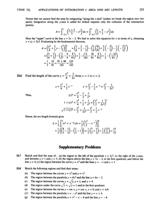
![256 APPLICATIONS OF INTEGRATION I: AREA AND ARC LENGTH [CHAP. 32
(h) The region between the curvesy = fi and y = x3.
(i) The region in the first quadrant between the curves4y +3x = 7 and y = x - ~ .
(j) The region bounded by the parabolas y = x2 and y = -x2 +6x.
(k) The region bounded by the parabola x = y2 +2 and the line y = x - 8.
(Z) The region bounded by the parabolas y = x2 - x and y = x - x2.
(m) The region in the first quadrant bounded by the curves y = x2and y = x4.
(n) The region between the curve y = x3and the lines y = -x and y = 1.
32.9 Find the lengthsof the followingcurves:
x4 1
8 4x2
(a) y = -+-from x = 1to x = 2.
(b) y = 3x - 2 from x = 0 to x = 1.
(c) y = x2I3from x = 1 to x = 8.
(d) x2/3+y2l3= 4 from x = 1to x = 8.
(4 Y = 15+7
4x from x = 1to x = 2.
(f) y = 3 &(3 - x) from x = o to x = 3.
(9)
(h)
x5 1
1
24xy = x4 +48 from x = 2 to x = 4.
y = 3 (1 +x2)3/2
from x = O to x = 3.
2
32.10 Use Simpson’s rule with n = 10to approximatethe arc length of the curve y =f(x) on the given interval.
(a) y = x2 on [O,13 (b) y = sin x on CO, n] (c) y = x3on CO,5)](https://image.slidesharecdn.com/problemscalculus-221128025033-038ef06f/85/problems-calculus-pdf-269-320.jpg)
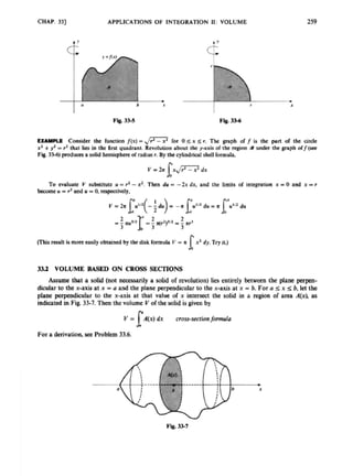
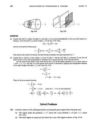
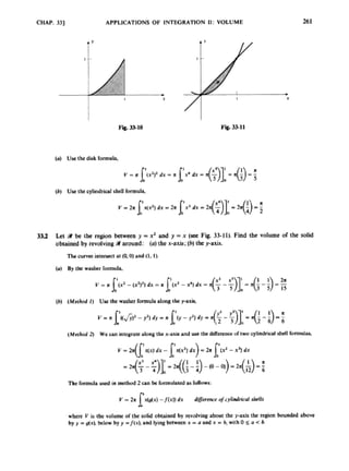
![262 APPLICATIONS OF INTEGRATION 11: VOLUME [CHAP. 33
33.3 Find the volume of the salid whose bax i
s a circle of radius I and such that every cross section
perpendicular to a particular fixed diameter D is an equilateral triangle.
Let the center of the circular base bc rhe origin. and let the x-axis he the diamcrer D. The a m of the
cross saclion at x isA(x)= hs/2{secFig 33-12). Now. in the horizontal right triangle,
and in the vertical right triungle,
h = Jsf -J5J-
Hcncc.A(x) = v/s(ra - x’ban cvcn function-and the cross-section formula gives
Fig, 3 sI2
33.4 Establish the disk formula V = R (((x))~ dx.
s:
We assume as valid the expression ir% fbr rhc volume of a cylinder d radius r and height h. Divide
the interval [a. b] into n qual subintemla each o
f length Ax -[h-o)/n(we Fig. 33-13). Consider the
volume V
, obtained by revolving the region d,above the ith subinterval about rhe x-axis. U mi and h4,
dcnotc the absolute minimum and the absolutc maximum dJon the Fbsutiritensl. it is plain that b: must
lie heirnen the rolumc of a cylinder or radiusm, and height Ax and the volumc of a cylinder or radius M,
and height Ax,](https://image.slidesharecdn.com/problemscalculus-221128025033-038ef06f/85/problems-calculus-pdf-275-320.jpg)
![CHAP. 331 APPLICATIONS OF INTEGRATION XI: VOLUME 263
Hence,
I
Sincethis relation holds(for suitable numbcnx
:
) for arbitraryA. it must holdin the limL as n +m
,
which is the disk formula. The name derives from the ux of cylindrical disks [ofthicknca Ax) to approx-
imate the V;.
Fig. 33-13 Fig. 33-14
3
3
5 Establish the cylindrical shell formula V = 2n xf(x) dx.
I'
Divide the interval [a, b] into n equal subintervals, each of length AV.
Ler 9,be the region abwc the
P" subinterval (secFig. 33-14). Letx
: be the midpoint ofthc Fbsubinterval. x
: -(.x,-, +n#2.
Now the solid obtained by revolving the region Yt
about the paxit is approximately the solid oblainud
by revolvingthc mangle with basc AYand height y
: =/(x:). The latter solid is a cylidrical Ml;that is.
i t is lhe difference between the cylinders obtained by rotating the rectangles with the same heigbtf[x:) and
with bares [O.x,- end [O. XJ H m .it has volume
A X ~ J ( X ~ )
- XX:- f(.~:)rt/(x:n~: -x
:
- 1) = M(x:Mx,+ x,- ~Mx, -x,- k)
= nf(x:W2x:HAx) = Znx:f(xf) Ax
Thusthe tau V is approximated by
2nEx:f(xf) Ax
x/(x) dx.
1 - 1
which in turn approximatmthe definiteintegral 2r
I'
33A Esmblish the cross-section formula V = A(x) dx.
I"
Divide the interval [a, h] into n equal wbmrerrab[x,_,,xi].each of length Ax. Choose a point x? in
[x,- ,,xJ. If n is larp, making Ax mall, the piox of the d i d between x, -,and x, will bc very nearly a](https://image.slidesharecdn.com/problemscalculus-221128025033-038ef06f/85/problems-calculus-pdf-276-320.jpg)
![264 APPLICATIONS OF INTEGRATION 11: VOLUME [CHAP. 33
(noncircular) disk, of thickness Ax and base area A(xF) (see Fig. 33-15). This disk has volume A(x:) Ax.
Thus,
Fig. 33-15
3
3
.
7 (Solids of Revolution about Lines Parallel to a Coordinate Axis) If a region is revolved about a
line parallel to a coordinate axis, we translate the line (and the region along with it) so that it
goes over into the coordinate axis. The functionsdefining the boundary of the region have to be
recalculated. The volume obtained by revolving the new region around the new line is equal to
the desired volume.
(a) Consider the region 9 bounded above by the parabola y = x2, below by the x-axis, and
lying between x = 0 and x = 1 [see Fig. 33-16(a)].Find the volume obtained by revolvingW
around the horizontal line y = -1
.
(b) Find the volume obtained by revolving the region W of part (a) about the vertical line
x = -2.
(a) Move W vertically upward by one unit to form a new region W*.
The line y = -1 moves up to become
the x-axis. W*is bounded above by y =x' +1 and below by the line y = 1. The volume we want is
obtained by revolvingW*about the x-axis. The-washerformula applies,
V = II ((x' + I)' - 1
'
) dx =II
I'
(b) Move W two units to the right to form a new region 9
2
' [see Fig. 33-16(b)]. The line x = -2 moves
over to become the y-axis. W x is bounded above by y = (x -2)' and below by the x-axis and lies
Y
I X
1
-
a
Y
1 2 3 x
Fig. 33-16](https://image.slidesharecdn.com/problemscalculus-221128025033-038ef06f/85/problems-calculus-pdf-277-320.jpg)
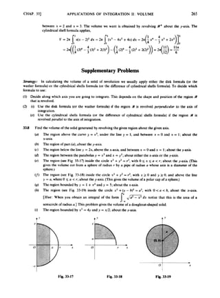
![266 APPLICATIONS OF INTEGRATION I1: VOLUME [CHAP,33
0
1 The region bounded by y =4/x and y -(x -3)z;about the x-axis. poticc that the curwca intersect
w h x = l a n d x = 4 . ~ 1 i s ~ l a b o u l 1 h e i n t e r s a c d o n a t x = l ? )
(k) The region of part 0;aboul he y-axis.
(0 The region bounded by xy = I. x = 1, x = 3. y =0: about the x-axis.
(m) The region ofp
a
n(0;about the y-axis.
UK the crmsiectionformula 10 Rad the volumc o
f the followingsolick
(U) The Wlid har 8 base which b a a r c k o
f radius r, Each m
s
)ssction perpendicularto a fixed diametet
of thecircle is an Lsorcelestrianglewith altitude equal tooae-haUofits base.
(b) Tbc solid is a wedge. cut from a pcriaCtly round trac o
f radius r by two planes, one perpendicular to
the axis ofthe I t e t m d the other inlensecting the first plane at an angle of W along a diameter (see
(4 A square pyramid with 8 heishtof h unitsa d a bortof Side r unira [Hint: Locate the x-axb 8s in F
i
g
.
33-21. By similarriglit ~riangks.
3
M
Pig, 33-20).
d h - x
-
I
-
e h
and
which &ermines A(xl.1
(4The tetrrhedron (see Fig. 33-22) formed by Ihroe mutually perpendicular CaccS and thm m u l d y
perpendicularedges o
flengthsn, b,c. [Hh:Another pyrsmid;proceed 85 in part (cl-]
I
TX
t X](https://image.slidesharecdn.com/problemscalculus-221128025033-038ef06f/85/problems-calculus-pdf-279-320.jpg)
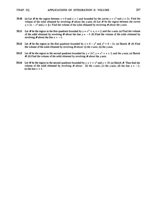
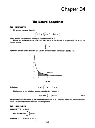
![CHAP. 341 THE NATURAL LOGARITHM 269
This is apparent from the area interpretation (Fig. 34-1)or, more rigorously, from Problem 30.11.
PROPERTY 3. If 0 c x < 1, In x < 0.
" 1 ' 1
In fact, In x = 7tit = - [- tit [reversing limits of integration]
t
and, for 0 c x < 1,
by Problem 30.11.
PROPERTY 4. - dx = In 1x1 +C [x # 0).
1:
In other words, In 1x1 is an antiderivative of x - l for all nonzero x. The proof is simple. When
x > 0, then 1x1= x, and so
When x <0, then 1x1 = -x, and so
D,(ln I x I) = D,(ln (-x)) = D,(ln u)D,(u) [by the chain rule; U = - x > O]
= (t>(-1)
PROPERTY 5. In uv = In U +In v.
For a proof, see Problem 34.2.
U
V
PROPERTY 6. In - = In U - In v.
U
V
Proof: In Property 5, replace U by -.
1
PROPERTY 7. In - = -In v.
Proof:
PROPERTY 8. For any rational number r, In x' = r In x.
V
Let U = 1 in Property 6 and use Property 1.
See Problem 34.3 for a proof.
PROPERTY 9.
Proof: Since D,(ln x) = - >0, In x must be an increasing function.
PROPERTY 10. In U = In D implies U = v.
In x is an increasing function.
1
X
This followsfrom Property 9. Since In x is increasing, it can never repeat a value.
PROPERTY 11. c In 2 c 1.](https://image.slidesharecdn.com/problemscalculus-221128025033-038ef06f/85/problems-calculus-pdf-282-320.jpg)
![CHAP. 343 THE NATURAL LOGARITHM 271
f'
Fig. 34-2
Then, by Theorem 30.4,
3
4
3 Prove: In x' = r In x for rational r.
By the chain rule,
Then, by Corollary 29.2, In x
'= r In x +C, for some constant C. Substituting x = 1, we find that C = 0,
and the proof is complete.
34.4 Evaluate:
(a) D,(h (x3 - 2x)) (b) D,(ln (sin x)) (c) Dices (In x))
Use the chain rule.
3x2-2
(3x2- 2) =-
1
Dx(x3- 2x) = - x3 - 2x
x3 - 2x
1
(a) D,(h (x3- 2x)) = -
x3 - 2x
(cos x) =-= cot x
(b) D,(ln (sin x)) = -D,(sin x) = -
1 sin (ln x)
(c) D,(cos (In x)) = -(sin (In x)) DJln x) = -(sin (In x)) - = - -
cos x
1 1
sin x sin x sin x
X X
34.5 Quick Formula 11: 1- dx = In If(x)l+ c.
*f'(x) D y the chain rule]
Proof: D,(ln If (x) I)= -
f(4
1
3
4
.
6 Find the following antiderivatives:](https://image.slidesharecdn.com/problemscalculus-221128025033-038ef06f/85/problems-calculus-pdf-284-320.jpg)
![CHAP. 341 THE I~ATURALLOGARITHM 273
1
34.9 Show that 1-- 5 In x 5 x - 1for x > 0
.
X
For x 2 1, note that l/t is a decreasing function on [l,
x] and, therefore, its minimum on [l,
x] is l/x
and its maximum is 1.Then, by Problem 30.3(c),
1
- (x - 1) I
In x =
X
1
l - - s l n x ~ x - l
X
Note that 1- l/x < In x < x - 1 for x > 1 by Problem 30.11. For 0 < x c 1
, - l/t is an increasing func-
tion on [x, 13. By Problem 30.3(c),
--(1
1 - x ) I l n x = [ S d t = [ (-:)dts -1(1 -x)
X
1
Hence,l - - l ; l n x < x - 1.
X
Supplementary
34.10 Find the derivatives of the following functions:
(a) In (4x - 1) (b) (In x ) ~ (c) 6
x - 1
(e)* x2 In x (f)In x+l (9) In I5x - 2I
Problems
34.11 Find the following antiderivatives. Use quick formula I1 whenever possible.
34.12 Use logarithmic differentiation to find y':
,/xL - 1 sin x
(c) =
(2x +3)4
34.13 (a) Show that In x < x. [Hint: Use Problem 34.9.1
In x 2
(b) Show that -<-. [Hint: Replace x by fiin part (a).]
x &
In x
(c) Prove: lim --
-0. [Hint: Use part (b).]
x + + m x](https://image.slidesharecdn.com/problemscalculus-221128025033-038ef06f/85/problems-calculus-pdf-286-320.jpg)
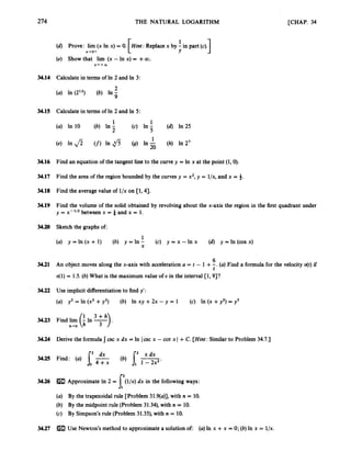
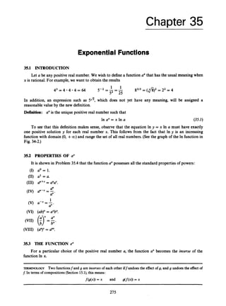
![276 EXPONENTIAL FUNCTIONS [CHAP. 35
Definition: Let e denote the unique positive real number such that
l n e = 1 (35.2)
Since the range of In x is the set of all real numbers, there must exist such a number e. It can be
shown that e = 2.718 ....[SeeProblem 35.3o(c).]
Tkorem 35.1: The functions e" and In x are inverses of each other:
In ex= x and elnx- x
-
Indeed, substituting e for U in (354,
In ex = x In e = x 1 = x
If we replace x in this result by In x,
In elnx= In x
Hence, ,1nx -
- x [since In u = In U implies u = U by Property 10, Section 34.21
Theorem 35.1 shows that the natural logarithm In x is what one would call the "logarithm to the
base e"; that is, In x is the power to which e has to be raised to obtain x: ,Inx -
- x.
Theorem35.2: ax= e"In '.
Thus, every exponential function a" is definable in terms of the particular exponential function ex,
which for this reason is often referred to as the exponential function. To see why Theorem 35.2 is true,
notice that, by Theorem 35.1,
In ex'"' = x In a
But y = uxis the unique solution of the equation In y = x In a. Therefore,
,xlna -
- ax
In Problem 35.9 it is shown that exis differentiable and that:
Theorem35.3: Dx(e")= ex.
Thus, ex has the property of being its own derivative. All constant multiples Ce"share this property,
since Dx(Cex)
= C Dx(ex)
= Ce". Problem 35.28 shows that these are the only functions with this
property.
From Theorem 35.3, we have
exdx = ex+ C (35.3)
s
Knowing the derivative of ex,we obtain from Theorem 35.2
D,(aX) = DX(ex'"')
= e"In' D,(x In a) [by the chain rule]
In a = axIn a
-
- ex In a .
This proves:
Theorem35.4:
or, in terms of antiderivatives, / a . dx = + c
We know that Dx(Y)= r$-' for any rational number T. Now the formula can be extended to
arbitrary exponents. If, in Theorem 35.2, we replace x by T and U by x (thereby making x positive), we
Dx(ax)
= (In a)ax
(35.4)
ax](https://image.slidesharecdn.com/problemscalculus-221128025033-038ef06f/85/problems-calculus-pdf-289-320.jpg)
![CHAP. 351 EXPONENTIAL FUNCTIONS 277
get x' = e'In ".Hence,
D,(xr) = D,(e' In = e
' In "D,(r In x) [by the chain rule]
Thus, we have the following:
Theorem 355: For any real number r and all positive x,
D,(x? = rxr-
Solved Problems
35.1 Evaluate: (a)e2In"; (b) In e2; (c)e('"")-';(d) 1".
(a) e2InX
= (e'"?' [by Property (VIII)]
(b) In e2= 2 [by Theorem 35.1)
(c) e('nU)- 1 = - [by Property (IV)]
= x2 [by Theorem 35.1)
U
e1
U
= -
e
[by Theorem 35.1 and Property (II)]
(d) By definition,In 1" = x(ln 1)= x(0)= 0 = In 1.Hence, 1" = 1.
35.2 Find the derivatives of: (a)e6; (b) 32";(c)xe"; (d) 3x3.
(a) Dx(e3= eJ;D,(&) [by the chain rule]
(b) D,(32? = (In 3)32x0d2x)
(c) D,(xe? = xD,(e? +DJx)ex [by the product rule]
[by the chain rule and Theorem 35.4)
= (ln 3)32x(2)= (2 In 3)32x
= xe" +( l w = ex(x+ 1)
(d) D"(3Xfi) = 3Dx(xJi) = 3 ( d x f i - I ) = 3JzxJi-1
353 Find the following antiderivatives (ex' stands for e("')): (a) 10" dx; (b) xe"' dx.
s I
(a) By Theorem 35.4,
I10" dx = 1w+c
Ixr"dx =; I e udu =?
1 e" +C = -
1 e2
+C
(b) Let U = x2.Then du = 2x dx, and
2](https://image.slidesharecdn.com/problemscalculus-221128025033-038ef06f/85/problems-calculus-pdf-290-320.jpg)
![CHAP. 351 EXPONENTIAL FUNCTIONS 279
(a) In y = In xx = x In x. Now differentiate,
In 2 1 In 2
+ 5 --x - w = -
1dy 1 1
ydx 2 x + 1 2
--=--
2(x + 1) +
-
1
dx = y ( m + 5 - 2J;;
35.7 Prove the followingfacts about ex:
ex >0 (b) ex is increasing (c) ex > x (d) lim ex = +a (e) lim ex = 0
ux> 0, by definition (Section 35.1).
Dx(e3= ex > 0, and a function with positive derivative is increasing. More generally, the definition of
a", together with the fact that In y is increasing, implies that axis increasingif U > 1.
We know (Problem 34.8) that In U < U. Hence, x = In ex < ex.
This is a direct consequenceof part (c).
Let U = -x; then, by Property (V),
X++OO x+-OO
As x + -00, U --* +00, and the denominator on the right becomes arbitrarily large [by part (d)].
Hence, the fraction becomes arbitrarily small.
35.8 Sketch the graph of y = ex, and show that it is the reflection in the diagonal line y = x of the
graph of y = In x.
From Problem 35.7 we know that ex is positive and increasing, and that it approaches + m on the
right and approaches 0 on the left. Moreover, since D;(e? = ex > 0, the graph will be concave upward for
all x. The graph is shown in Fig. 35-l(a).
By Theorem 35.1, y = ex is equivalent to x = In y. So, a point (a, b) is on the graph of y = ex if and
only if (b, a) is on the graph of y = In x. But the points (a, b) and (b, a) are symmetricwith respect to the line
y = x, by Problem 6.4.
In general, the graphs of any pair of inverse functions are mirror images of each other in the line y = x.
35.9 Prove: (a) ex is continuous (6) ex is differentiable,and &(ex) = ex
Let E > 0. To prove continuity at x, we must show that there exists S > 0 such that IU - x I < 6 implies
Ie" - exI < E. Let E, be the minimum of ~ / 2
and 8/2. SinceIn is increasingand continuous, the range of
In on (ex - E,, ex +E ~ )
is an interval (c, d) containing x. Let 6 > 0 be such that (x - 6, x +6) is
included within (c, d). Then, for any U, if IU - x I < 6, it follows that I e" - exI < E, < E.
The proof will consist in showing that
e X + h - 8
lim -
= ex
h+O](https://image.slidesharecdn.com/problemscalculus-221128025033-038ef06f/85/problems-calculus-pdf-292-320.jpg)
![CHAP. 351 EXPONENTIAL FUNCTIONS 281
(iii) ex - 6e-" = 5
e2x - 6 = Sex [multiply by 81
e2x- 5e" - 6 = 0
(ex -6Xex + 1) = 0
e x - 6 = 0 or e x + l = O
ex = 6
x = I n 6
[ex + 1 > 0, since ex > 01
[e" = b implies u = In b]
SupplementaryProblems
35.11 Evaluate the followingexpressions:
(a) ,-Inx (b) In e-x (c) (e4)lnx (d) (3eYnX
(e) e l n ( X - l ) (f) In (f) (9) eln(2x) (h) In fi
35.12 Calculate the derivativesof the followingfunctions:
ex
(a) e-x (b) e"" (c) ecosx (d) tan ex (e) ;
(f)ex In x (9) x" (h) nx (i) In e2x U) ex - e-x
35.13 Evaluate the following antiderivatives:
r r r
(a) J e3x dx
(d) Jecosxsin x dx
(b) J eexdx
(e) J32x dx
(c) J e x d F Z dx
e2x
(h) dx (i) dx
(
J 1x22" dx (k) 1 x 3e-x4 dx
35.14 Use implicit differentiation to find y':
(a) ey = y +In x (b) tan ey-x = x2 (c) elly +ey = 2x
(d) x2 +exY +y2 = 1 (e) sin x = e
Y
35.15 Use logarithmic differentiation to find y':
(d) y = (In x)'" (e) y2 = (x + 1Xx +2)
(a) y = 3 S i " X (4 Y = (J2)C' (c) y = XInx
35.16 Solve the followingequations for x:
(a) e3x = 2 (b) In x3 = - 1 (c) ex - 2e-" = 1 (d) In (In x) = 1 (e) In (x - 1) = O
35.17 Consider the region 9 under the curve y = ex, above the x-axis, and between x = 0 and x = 1. Find:
(a) the area of 9;(b) the volume of the solid generated by revolving 9 about the x-axis.
35.18 Consider the region B bounded by the curve y = e"'2, the y-axis, and the line y = e. Find: (a) the area of
9 ;(b) the volume of the solid generated by revolving 3about the x-axis.](https://image.slidesharecdn.com/problemscalculus-221128025033-038ef06f/85/problems-calculus-pdf-294-320.jpg)
![282 EXPONENTIAL FUNCTIONS [CHAP. 35
35.19 Let 9 be the region bounded by the curve y = ex', the x-axis, the y-axis, and the line x = 1. Find the
volume of the solid generated by revolving 9 about the y-axis.
35.20 Find the absolute extrema of y = 8'"
"on the interval [-n, n]. [Hint: euis an increasingfunction of u.]
35.21 If y = enx,where n is a positive integer,find the nth derivativey(").
35.22 Let y = 2 esin .(a)Find y' and y". (b) Assume that x and y vary with time and that y increases at a constant
rate of four units per second. How fast is x changing when x = n?
35.23 The acceleration of an object moving on the x-axis is 9e3'. (a)If the velocity at time t = 0 is four units per
second, find a formula for the velocity dt).(b) How far does the object move while its velocity increases
from four to ten units per second? (c) If the object is at the origin when t = 0, find a formula for its position
x(t)-
35.24 Find an equation of the tangent line to the curve y = 2e" at the point (0,2).
35.25 Sketch the graphs of the followingfunctions,indicating relative extrema, inflection points, and asymptotes:
(a) y = e-"' (b) y = x In x
In x
(4 Y = x
1
(6) y = e - " (e) y = ( I - l n ~ ) ~ (f)y = ; + l n x
[Hint: For parts (b)and (c) you will need the results of Problem 34.13(d)and (c).]
35.26 Sketch the graphs of y = 2" and y = 2-". [Hint: a" = exIn ".]
In x
-. This function is called the logarithm ofx to the base a (log,, x is
In a
35.27 For a > 0 and a # 1, define log,x
called the cornon logarithm ofx). Prove the following properties:
(b) alofi" = x
1
x In a
(a) D,(lOg, x) = - (c) log, a" = x
U
U
(d) log, x = In x (e) log,, (uu) = log, U +log, U (f) log, - = log, U -log,, U
log, x
(9) log, U
' = r log, U (h) In x = -
log, e
35.28 Show that only the functionsf(x) such thatf'(x) =f(x) are the functions Ce",
where C is a constant. [Hint:
Let F(x) =f(x)/ex and find F'(x).]
35.29 Find the absolute extrema off(x) = (In x)'/x on [l, e].
35.30 (a) Prove ex = lim (1 +E)". [Hint: Let y = (1 +f)'. Then,
Y * + W
[by the mean-value theorem]
1
= u ( l n ( u + x ) - l n u ) = u - x * -
U*
U* X
where U < U* < U +x if x > 0, and U +x < U* < U if x < 0. Then either 1 <-< 1 +- if x > 0 or
1 + <-< 1 if x < 0. In either case, lim -= 1. So, lim In y = x and, therefore, lim y =
U U
x U* U*
U Y * + W U U++Q) U * + c O
1
lim eInY = ex.
U * + W](https://image.slidesharecdn.com/problemscalculus-221128025033-038ef06f/85/problems-calculus-pdf-295-320.jpg)
![CHAP. 351 EXPONENTIAL FUNCTIONS 283
(b) Prove e = lim .[Hint: Use part (a).]
n + + w
(c) rnApproximate e by finding (1 +(t)rfor large values of n (say,n 2 10OOo).
X"
3531 Show that, for any positive n, lim -= 0.
x-, +w ex
1
1 1
Hint: -= -- -
=
ex -
In ex'l- Inxlx). Now apply Problems 34.13(c)and 35.7(d).
-
35.32 Evaluate the following definiteintegrals:
1
35.33 Evaluate lim - (ell"+elln + - +enln).
n + + w n
35.34 Show that e" > ne. [Hint: Prove generally that U' > U" when U > U 2 e. (u/e)"-"2 1 since u/e 2 1 and
U > U. so,
u'e" 2 e'u" (1)
U u u U ue ue
By Problem 34.9, - - 1 > In -, - > In - + 1 = In -, e'/" > -, and so,
U u u U U U
By (1) and (2),u'e" > e"u", U' > U".]
3535 If interest is paid at r percent per year and is compounded n times per year, then P dollars become
P(1+-lknrdollars after 1 year. If we let n -+ 00, then the resulting interest is said to be continuously
compounded.
(a) Show that, if continuously compounded at r per cent per year, P dollars become Pe' dollars after 1
year. [Hint: Use Problem 35.30.1 Then, after t years, P dollars would become Per' dollars.
(b) Continuously compounded at 6 percent per year, how long would it take to double a given amount of
money?
(c) rnWhen r = 5 percent, compare the result of continuous compounding with that obtained by com-
pounding once a year and with that obtained by compounding monthly.
35.36 Use Newton's method to approximate a solution of: (a)ex = l/x; (b) e-x = In x.
35.37 Use Simpson's rule with n = 4 to approximate e-xz/2dx.
Jr,'](https://image.slidesharecdn.com/problemscalculus-221128025033-038ef06f/85/problems-calculus-pdf-296-320.jpg)
![Chapter 36
L’HGpital’s Rule;ExponentialGrowth and Decay
36.1 L’HOPITAL’S RULE
The followingtheorem allows us to compute limits of the form
in the “indeterminate case” when the numeratorf(x) and the denominator g(x) both approach 0 or both
approach fCO.
Theorem 36.1 (L‘H6pital‘sRule): Iff(x) and g(x) either both approach 0 or both approach & 00, then
In L’H6pital’s rule, the operator “lirn” stands for any of
lim lim lim lim lim
See Problem 36.21 for a sketch of the proof. It is assumed in Theorem 36.1 that g(x) # 0 and g’(x) # 0
for x sufficientlyclose to a.
X++CCl x+-CCl x-a x-a+ x-+a-
EXAMPLES Let us verify L‘Hbpital’s rule for four limits found earlier by other means.
(a) See Problem 9 4 4 ,
6x 6 6 3
,,-,4x2+5 x-r-,8x x+-,8 8 4
- ]im - = lim - = - = -
3x2 - 5
lirn --
(b) See Problem 27.4,
sin 8 cos e
lim -= lim --
- cos 0 = 1
e-ro 8 e-ro 1
(c) See Problem 34.13(4. To apply Theorem 36.1, we must rewrite the function as a fraction that becomes indeter-
minate,
In x X - ’
lim (x In x) = lim -
1
= lim - [Dx(ln x) = x-’]
X‘O+ X‘O+ x x-ro+ -x-2
= lim - x
X‘O+
= o
(d) See Problem 35.31, where now n is supposed to be an integer. By L‘H6pital’s rule,
X” nx”-
x++, ex X’+Co ex
lim - = lim -
As the right side is indeterminate, L’H6pital’s rule can be applied again,
nx”- n(n - I)x”-~
lirn -- - lim
e”
x + + w e“ X’+al
Continuing in this fashion, we reach, after n steps,
n(n - 1) ..-(2x1) 1
lim = n! lirn - = n ! ( 0 ) = 0
X - r + a , ex X’+, ex
284](https://image.slidesharecdn.com/problemscalculus-221128025033-038ef06f/85/problems-calculus-pdf-297-320.jpg)
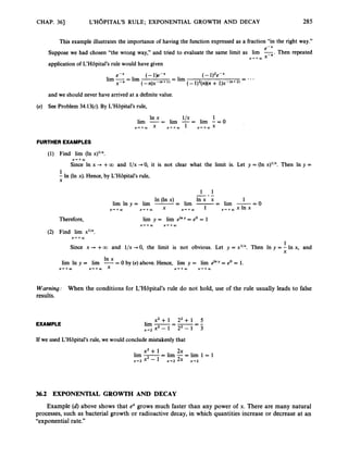
![286 L'HOPITAL'S RULE; EXPONENTIAL GROWTH AND DECAY [CHAP. 36
Definition: Assume that a quantity y varies with time t. Then y is said to grow or decay exponentially if
its instantaneous rate of change (Chapter 19) is proportional to its instantaneous value;
that is,
* = K y
dt
(36.2)
where K is a constant.
Suppose that y satisfies(36.1).Let us make the change of variable U = Kt. Then, by the chain rule,
dy dydu - d ~ K or - = y
dY
du
K Y = - = - - - -
dt du dt du
and so, by Problem 35.28,
y = Ce" = CeKt (36.2)
where C is another constant.
We can now see why the process y is called exponential. If K > 0, K is called a growth constant, and
y increases exponentially with time. If K < 0, K is called a decay constant, and y decreases exponentially
with time.
Let y, be the value of y at t = 0. Substituting 0 for t in (36.2),we obtain
y, = Ceo = C(1) = C
so that (36.2)can be rewritten as
y = y,eK' (36.3)
EXAMPLES
(a) Assume that a culture consisting of loo0 bacteria increases exponentially with a growth constant K = 0.02,
where time is measured in hours. Let us find a formula for the number y of bacteria present after t hours, and
let us compute how long it will take until 1
O
O
O
O
Obacteria are present in the culture.'
Since y, = 10o0, the desired formula for y is given by (36.3),
y = 1O()OeO.O2*
Now set y = 1
O
O
O
O
Oand solve for t,
1OOOOO = 1000e0*02'
100 = eo.02*
In 1
O
O = In eo.OZ'
2 In 10 = 0.02t pn 10' = 2 In 10; In e" = U]
t = 100 In 10
Appendix E gives the approximate value of 2.3026for In 10.Thus,
t x 230.26 hours
Note: Sometimes, instead of specifying the growth constant K,say, K = 0.02, one says that the quantity is
increasing at the rate of 2 percent per unit time. This is not quite accurate. A rate of increase of r percent per
unit time is approximately the same as a value of K = O.Or when r is relatively small (say, r 5 3). In fact, with
Although populationsare measured in positiveintegers, (36.3)seems to be applicable, even though that formula was derivedfor
a quantity measuredi
n real numbers.](https://image.slidesharecdn.com/problemscalculus-221128025033-038ef06f/85/problems-calculus-pdf-299-320.jpg)
![CHAP. 363 L'H~PITAL'SRULE; EXPONENTIAL GROWTH' AND DECAY 287
an r percent growth rate, y = yo(l +O.Or) after one unit of time. Since y = yoeK when t = 1, eR= 1 +O.Or,
and, therefore, K = In (1 +0.Or). This is close to O.Or, since In (1 +x) x x for small x. [For example,
In (1.02) x 0.0198 and In (1.03) x 0.02956.1 Thus, many textbooks will automatically interpret a rate of
increase of r percent per unit time to mean that K = O.Or.
If the decay constant of a given radioactive element is K < 0, compute the time T after which only half of any
original quantity remains.
At t = T, (36.3)gives
- I n 2 = K T I n - = - l n x
[
I 1
In 2
K
--- - T (36.4)
The number T is called the half-life of the given element. Knowing either the half-life or the decay constant, we
can find the other from (36.4).
Solved Problems
(In x)"
36.1 Show that lim --
- 0 for any positive integer n.
Y
The proof will proceed by mathematical induction (see Problem 12.2).The assertion is true for n = 1,
by Problem 34.13(4. Assuming that it is true for n = k, we have, for n = k + 1,
(In x ) ~
+ (k + lMln x)~x-
lim -- - lim I [by L'H8pital's rule]
Thus, the assertion is also true for n = k + 1,and the proof is complete.
ex - 1
x+o sin x
3
6
.
2 Find lim -.
The numerator and the denominator are continuous functions, each 0 at x = 0. Therefore, L'Hbpital's
rule applies,
e0 1
- --- - = 1
ex - 1 ex
lim --
- lirn --
x+o sin x x+o cos x cos0 1](https://image.slidesharecdn.com/problemscalculus-221128025033-038ef06f/85/problems-calculus-pdf-300-320.jpg)
![CHAP. 361 L'HOPITAL'S RULE; EXPONENTIAL GROWTH AND DECAY 291
3
6
.
2
0 Prove Cauchy's extended mean-value theorem: If f and g are differentiable in (a, b) and continuous on
[a, b],and ifg'(x) # 0 for all x in (a, b),then there exists a point c in (a, b)such that
[Hint:
Apply the generalized Rolle's theorem (Problem 17.19)to
h(x) = (f(b) -f(a))g(x) - (g(b)- s(a))f(x)
Note that g(b) # g(a) since,otherwise, the generalized Rolle's theorem would imply that g'(x) = 0 for some x
in (a, b).)
36.21 Prove L'H6pital's rule. [Hint:
Consider the case lim,,,+ (f(x)/g(x)),
where lim,,,, f ( x ) = lirn,,,, g(x)= 0.
We may assume that f(a) = g(a) = 0. Then, by Problem 36.20, f(x)/g(x)= ( f ( x )-f(a))/
@(x) -g(a))=f'(x*)/g'(x*) for some x* between a and x. Therefore, as x + U + , x* -11'. Hence, if
(f'(x)/g'(x))= L, then lim,,,, (f(x)/g(x))= L. The other cases can be handled in the same way or
can be reduced to this case.]](https://image.slidesharecdn.com/problemscalculus-221128025033-038ef06f/85/problems-calculus-pdf-304-320.jpg)
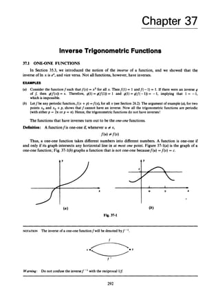
![CHAP. 371 INVERSE TRIGONOMETRIC FUNCTIONS 293
If a one-one function f is defined by means of a formula, y =f(x), we can sometimes solve this
equation for x in terms of y. This solution constitutes the formula for the inverse function, x =f-'(y).
EXAMPLES
(a) Letf(x) = 3x + 1(a one-one function). Let y stand forf(x); then y = 3x + 1. Solve this equation for x in terms
of Y,
y - l = 3 x
--
Y - L x
3
Therefore,the inversef-' is given by the formula
Y-1
f-'(y) = -
3
(6) Consider the one-one functionf(x) = 2e" - 5,
y = 2e" - 5
y +5 = 2e"
Y + 5
2
-- - ex
Y + 5
In -= In ex = x
2
Thus,
(c) Let f(x) = xs +x. Sincef'(x) = 5x4+ 1 > 0,f is an increasing function, and therefore one-one (see Problem
37.12). But if we write y = xs +x, we have no obvious way of solving the equation for x in terms of y.
37.2 INVERSES OF RESTRICTED TRIGONOMETRIC FUNCTIONS
restricted to some subset of one period.
For a periodic function to become one-one-and so to have an inverse-its domain has to be
Inverse Sine
The domain off(x) = sin x is restricted to [-4 2 , 421, on which the function is one-one [in fact,
increasing; see Fig. 37-2(a)]. The inverse function f - '(x) = sin- 'x is called the inverse sine of x (or,
sometimes, the arc sine of x, written arc sin x or arcsin x). Its domain is [-1, 13.Thus,
tY
( a ) y = sin x
Fig. 37-2
(b) y = sin-'x](https://image.slidesharecdn.com/problemscalculus-221128025033-038ef06f/85/problems-calculus-pdf-306-320.jpg)
![294 INVERSE TRIGONOMETRIC FUNCTIONS [CHAP. 37
The graph of sin-' x is given in Fig. 37-2(6). By a general theorem, the inverse of an increasing
function is itself an increasing function. You will find it helpful to think of sin- ' x as the angle (between
-n/2 and 4 2 ) whose sine is x.
EXAMPLES
1 a
2 6
fi a (4 sin-'-=-
(c) sin-' -= -
2 4
a J s a
(a) sin-' 1 = - (b) sin-' -= -
2 2 3
n n
(e) sin-' 0 = 0 (f)sin-l( - i)= - - (g) sin-'( - 1) = - -
6 2
The derivative of sin-' x may be found by the general method of Problem 35.9(6).In this case, a
shortcut evaluation is possible, using implicit differentiation. Let y = sin- ' x. Then,
sin y = x
d d
-(sin y) = -(x)
dx dx
dY
(cos y) -= 1 [by the chain rule]
dx t
dy 1
-1 1
-
_ -
-
dx cos Y + J i T F y = +JS
where the positive square root is implied because cos y > 0 for -n/2 < y < 4 2 . Thus we have found
dx = sin-' x +C
1 1
DJsin - x) =
Jc7 (37.1)
The importance of the inverse sine function in calculus lies mainly in the integration formula (37.1).
The procedure for the other trigonometric functions is exactly analogous to that for the sine func-
tion. In every case, a restriction of the domain is chosen that will lead to a simple formula for the
derivative of the inverse function.
Inverse Cosine (Arc Cosine)
(a) y = COS% (b) y =cos-'x
Fig. 37-3](https://image.slidesharecdn.com/problemscalculus-221128025033-038ef06f/85/problems-calculus-pdf-307-320.jpg)
![CHAP.371 INVERSE TRIGONOMETRIC FUNCTIONS 295
y=cosx [ O I x 1 a ] e> x=cos-'y [ - 1 I y I 1 ]
Interpret cos-' x as the angle (between0 and II)
whose cosine is x. Let y = cos-' x. Then,
cos y = x
&(cos y) = D,(x) = 1
* d
Y
- m y - = 1
dx
Note that sin y = +,/1 - cos2y since sin y > 0 when 0 < y < a. Thus,
dx = -COS-' x +C
1 1
D,(cos-' x) = -
Ji=7
Observe that - cos-' x and sin-' x have the same derivative;see Problem 37.17.
Inverse Tangent (Arc Tangent)
(a) y = tan x
iII
(b) y = tan-'x
Fig. 37-4
(37.2)
Interpret tan-' x as the angle (between -a/2 and z/2) whose tangent is x. Let y = tan-' x. Then,
tan y = x
D,(tan y) = 1
d
Y
sec2y -= 1
dx
1
--
-
1
-
d
Y 1
----
-
dx sec2y 1+tan2 y 1 +x2
Thus, dx = tan-' x +C
1 and 1-1
&(tan-' x) = -
1 + x 2 1 + x 2
(37.3)](https://image.slidesharecdn.com/problemscalculus-221128025033-038ef06f/85/problems-calculus-pdf-308-320.jpg)
![296 INVERSE TRIGONOMETRIC FUNCTIONS
- 1
Inverse Cotangent (Arc Cotangent)
I
Y
(a) y = c o t x (6) y = cot-'x
Fig. 37-5
y = c o t x [ O < x < n ] - x=cot-'y [ally]
Interpret cot-' x as the angle (between0 and n)whose cotangent is x. Then,
dx = -cot-' x +c
1
DJcot-' x) = --
1 +x2 Or
For the relation between cot-' x and tan-' x, see Problem 37.17.
Inverse Secant(Arc Secant)
I
I
-
I - I
I
I
I
I
I
I
I
I
I
Y
)I
I
I
I
I
I 1
I
w 3
x
;;
-X
[CHAP. 37
(37.4)
W
f
I
(6) y = sec-'x
X
( a ) y =secx
Fig. 37-6](https://image.slidesharecdn.com/problemscalculus-221128025033-038ef06f/85/problems-calculus-pdf-309-320.jpg)
![CHAP. 371 INVERSE TRIGONOMETRIC FUNCTIONS 297
The secant function is restricted to two separate subintervals of the fundamental period
(-71/233 7 m ,
0I x < 71/2
y=secx [or ] e> x=sec-'y [Iy( 2 11
71 I x < 37112
Interpret sec-' x as the angle (in the first or third quadrant) whose secant is x. Then,
dx = sec-' x +C
1 1
Dx(sec-' x) =
X J Z T
See Problem 37.7.
Inverse Cosecant (Arc Cosecant)
(37.5)
( U ) y = cscx
Fig. 37-7
1 I 1 L
(6)y = csc-' x
0< x I71/2
y=cscx [or ] * x=csc-' y [IyI 2 13
?I < x I 37112
Interpret csc-' x as the angle (in the first or third quadrant) whose cosecant is x. Then,
dx = -csc-' x +c
1 1
Dx(csc-'x) = -
X J Z i
For the relation between csc-' x and sec-' x, see Problem 37.17.
(37.6)](https://image.slidesharecdn.com/problemscalculus-221128025033-038ef06f/85/problems-calculus-pdf-310-320.jpg)
![298 INVERSE TRIGONOMETRIC FUNCTIONS [CHAP. 37
SolvedProblems
37.1 A one-one function has an inverse. Prove, conversely, that a function with an inverse is one-one.
If the domain off consists of a single point, there is nothing to prove. Let f have the inverse g, but
suppose, contrary to hypothesis, that the domain off contains two distinct numbers, U and U, such that
f(u) =f(v).Then,
= g(f(u)) = g(f(d) = "
a contradiction. We must then admit thatf(u) #f(o); that is, thatfis one-one.
37.2 Determine whether each of the following functionsfis one-one. If it is one-one, find a formula for
its inversef - '.
(a) f ( x ) = x2 +6x - 7 (6) f ( x ) = In (x2 + 1) (c) f ( x )= 5x3 -2
b)f ( x )= x2 +6x +7 = (x +7)(x - 1).Becausef( -7) = 0 =f(l),fis not one-one.
(4Obviously,f( +1)=f(-1);fis not one-one.
(c) If y = 5x3 - 2, then,
y +2 = 5x3
--
y + * - x 3
5
Thus,f(x) = 5x3 - 2 has an inverse,
f-'(y) = 3 Y
J ;*
and so, by Problem 37.1,fis one-one.
37.3 Find formulas for the inverses of the following one-one functions:
(a) f ( x )= 1Ox - 4 (6) f ( x )= 3e" + 1
(a) Let y = 1Ox - 4. Then,
- x
Y + 4
y+4=1Ox or --
10
Y + 4
f-'(J) = -
10
Hence,
(b) Let y = 3e" + 1.Then,
y - 1 =3ex or -- - e x or In --
Y - L
3
Y-1
3
Y-1
f-'(y) =In -
3
Hence,
37.4 Find the following values:
(a) sin-' (-k) (6) cos-' (-k) (c) tan-' (-1)
a n 1 A
(a) sin-' (-5)= the angle in [- 5,T] whose sine is -- = - -
2 6 '](https://image.slidesharecdn.com/problemscalculus-221128025033-038ef06f/85/problems-calculus-pdf-311-320.jpg)
![CHAP. 371 INVERSE TRIGONOMETRIC FUNCTIONS 299
1 a 5n
(b) cos- '(-i)= the angle in [0, a] whose cosine is - - -
(c) tan- '(- 1)= the angle in (-;
, ;
) whose tangent is -1 = --
4 '
2 - -6 = 6'
a
37.5 Evaluate: (a)cot-' fi;(6)sec-' 2; (c)csc-' (2/fi).
(a) cot-' fi is the angle 8between 0 and a such that cot 8 = fi.This angle is a/6 (see Fig. 37-8). Note
that an inverse trigonometric function must be represented by an angle in radians.
(b) The angle 8 whose secant is + 2 must lie in the first quadrant. The secant function is negative in the
third quadrant. From Fig. 37-8,8 = a/3.
(c) The angle 8 whose cosecant is + 2 / f i must lie in the first quadrant. The cosecant function is negative
in the third quadrant. From Fig. 37-8,8 = a/3.
Fig. 37-8
37.6 Find the derivatives of:
X
(a) sin-' 2x (6) cos-' x2 (c) tan-' - (d) sec-' x3
2
Dx(2x) [by the chain rule]
1
J
W
Ji=G JGG
J
-
(a) D,(sin-' 2x) =
1 2
(2) =
-
-
- 1
(b) DJCOS- 'x2) = Dx(x2) [by the chain rule]
- 1 -2x
(2x) = -
=
-
Ji=7 JD
1
D(;) [by the chain rule]
4 1
1+- 1+-
4
Dx(x3) [by the chain rule]
1
(d) DJsec - 'x3)=
x3J-
3
(3x2)=
1
-
-
x 3 J G X p T](https://image.slidesharecdn.com/problemscalculus-221128025033-038ef06f/85/problems-calculus-pdf-312-320.jpg)
![300 INVERSE TRIGONOMETRIC FUNCTIONS [CHAP. 37
1
3
7
.
7 Assuming that sec-' x is differentiable,verify that Dx(sec-' x) =
xJ.T-1'
Let y = sec-' x. Then,
s e c y = x
&(sec v)= 4 ( x )
dY
dx
dY
dx sec y tan y x tan y
(sec y tan y ) -= 1 [by the chain rule]
1
--
-
1
-
--
But the identity 1 +tan' y = sec2y gives
1 +tan2 y = x2 or tan2 y = x' - I or tan y = +JZi
By definition of sec-' x, the angle y lies in the first or third quadrant, where the tangent is positive. Hence,
1
-
dY
tan y = +
,
/
- and --
dx xJ;;i_l
3
7
.
8 Prove the followingformulas for antiderivatives:
1 X
a' +x2 a a
(a) J'L
= - tan-' - + c
NOTATION It is common to write
In each case, we employ the chain rule to show that the derivative of the function on the right is the
integrand on the left.
1 1 1
a
' x2 a2 +x'
=--=-
l + T
a](https://image.slidesharecdn.com/problemscalculus-221128025033-038ef06f/85/problems-calculus-pdf-313-320.jpg)
![CHAP. 371 INVERSE TRIGONOMETRIC FUNCTIONS 301
37.9 Find the following antiderivatives:
(a) By Problem 37.8(a), with a = 2,
(b) By Problem 37.8(b), with a = 3,
dx X
3
1 = sin- 1 -+c
(c) Complete the square: x2 +4x +5 = (x +2)2+ 1. Thus,
dx
Let U = x +2. Then du = dx, and
(d) Complete the square: x2 - 2x +7 = (x - 1)' +6. Let U = x - 1, du = dx, 2x = 2u +2. So,
f x 2 T t + 7 u 2 + 6
= s-2u +2 du = 1
m
2u du +1%
= In (
U
' +6) +2 -
2 x - 1
=In (x2 - 2x +7) +-tan-' -
U
[by quick formula I1 and Problem 37.8(a)]'
1
fi
37.10 Evaluate sin (2 cos- (- 4)).
Let 8 = cos-' (-4). Then, by Theorems 26.8and 26.1,
sin 28 = 2 sin e COS e = 2(fJi -COS2 excos e)
By definition of the function cos-', angle 8 is in the second quadrant (its cosine being negative), and so its
sine is positive. Therefore, the plus sign must be taken in the above formula,
We have written In (u2 +6) instead of In Iu2 +6 Ibecauseu2 +6 >0.](https://image.slidesharecdn.com/problemscalculus-221128025033-038ef06f/85/problems-calculus-pdf-314-320.jpg)
![302 INVERSE TRIGONOMETRIC FUNCTIONS [CHAP. 37
37.11 Show that sin-' x and tan-' x are odd functions.
More generally, we can prove that if a one-one function is odd (as are the restricted sin x and the
restricted tan x, but not the restricted cot x), then its inverse function is odd. In fact, iffis an odd one-one
function and g is its inverse, then
g(-f(x)) = s(f(
-x)) [sincef(4= -f(-41
= -x
= -g(f(x))
[since g is inverse off]
[since g is inverse off]
which shows that g is odd. (Could a one-one function be euen?)
Supplementary Problems
37.12 For each of the following functionsf, determine whether it is one-one; and if it is, find a formula for the
inversefunctionf - '.
37.13 Evaluate :
(6) tan-' -
3
3
37.14 (a) Let 8 = cos- '(4). Find the values of sin 8, tan 8, cot 8, sec 8, and csc 8.
(b) Let 8 = sin- ' (- 4). Find cos 8, tan 8, cot 8, sec 8, and csc 8.
37.15 Compute the following values:
(a) sin cos-' -
( :> (e) sin-' (sin n)
[Hints: Part (b)52 + 122= 132;part (c) cos (U +U ) = cos U cos U - sin U sin U ; part (e)is a trick question.]
37.16 Find the domain and the range of the functionf(x) = cos (tan- 'x).
37.17 Differentiate:
1
(a) sin-' x +cos-' x (b) tan-' x +cot-' x (c) sec-' x +csc-' x (6) tan-' x +tan-' -
(e) Explain the significance of your answers.
X](https://image.slidesharecdn.com/problemscalculus-221128025033-038ef06f/85/problems-calculus-pdf-315-320.jpg)
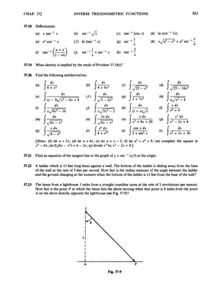
![304 INVERSE TRIGONOMETRIC FUNCTIONS [CHAP. 37
1
37.24 Find the area under the curve y = -
above the x-axis, and between the lines x = 0 and x = 1.
1 + x 2
above the x-axis,and between the lines x = 0 and x = 1/2.
37.25 Find the area under the curve y = -
1
Ji=7
1
37.26 Tine region 9 under the curve y = ~ above the x-axis, and between the linesx = 2 / f i and x = 2,
X2. f i
is revolved around the y-axis. Find th; volume of the resultingsolid.
37.27 Use the arc-length formula (32.2) to find the circumferenceof a circle of radius r. [Hint: Find the arc length
of the part of the circle x2 +y2 = r2 in the first quadrant and multiply by 4.1
37.28 A person is viewing a painting hung high on a wall. The vertical dimensionof the painting is 2 feet and the
bottom of the painting is 2 feet above the eye level of the viewer. Fiild the distance x that the viewer should
stand from the wall in order to maximizethe angle 8 subtended by the painting. [Hint: Express 8 as the
differenceof two inverse cotangents;see Fig. 37-10.]
X
Fig. 37-10
37.29 For which values of x is each of the followingequationstrue?
(a! sin-' (sin x) = x (b) cos-' (cos x) = x (c) sin-' (-x) = -sin-' x
(6) sin (sin-' x) = x (e) cos (cos-' x) = x
(J^)
Part (4
Use a graphing calculator to draw the graph of y = sin-' (sin x) and review your answer to
3730 Find y' by implicit differentiation:
(a) x2-- x tan-' y =In y (b) cos-' xy = e2Y
3731 Sketch the gaph of y = tan-' x - In J1 +x2.
3732 Assuming that cot-' x and csc-' x are differentiable,use implicit differentiationto derive the formulas for
their derivatives.
1
3733 Find the averagevaluesoff(x) = -
+ x2 on [-2,21.
37.34 (a) Show that IC = (b) ApproximateIC by applyingSimpson's rule to the definite integral in part
(a),with n = 8.](https://image.slidesharecdn.com/problemscalculus-221128025033-038ef06f/85/problems-calculus-pdf-317-320.jpg)

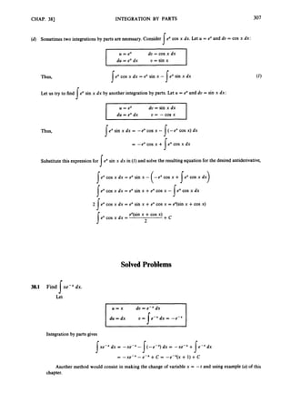
![308 INTEGRATION BY PARTS
38.2 (a) Establish the reductionformula
x"exdx = x"e" -n xn-'eX dx
s s
[CHAP. 38
(2)
for xnexdx (n = 1,2, 3, ...).
s
(4 Let
U = x" du = ex dx
and integrate by parts,
x " 8 dx = Yex - ex(nx"-')dx = x"8 - n x"-'ex dx
s s s
s s
s
(b) For n = 1, (2)gives
xe" dx = xe" - ex dx = xex - ex = (x - 1)ex
as in example (a).We omit the arbitrary constant C until the end of the calculation.Now let n = 2 in (2),
x2ex dx = x2ex- 2 xex dx = x2e"- 2((x - 1)eX)
= (x2 - 2(x - l)P= (x2 - 2x +2)e" +c
3
8
.
3 Find tan'' x dx.
Let
s
I
I u=tan" x d u = d x
du = -dx u = x
I 1 +x2
Hence,
X
tan-' x dx = x tan-' x - -
J 1 +x2 dx
=xtan-l x - - 1-
2x dx
J
2 1 + x 2
1
= x tan-' x -- In II +x21+ C
2
1
= x tan-' x -- In (1 +x2) + C
2
38.4 Find cos2 x dx.
Let
s
[by quick formula 11, Problem 34.53
[since 1 +x2 > O]
du = - sin x dx U = sin x](https://image.slidesharecdn.com/problemscalculus-221128025033-038ef06f/85/problems-calculus-pdf-321-320.jpg)
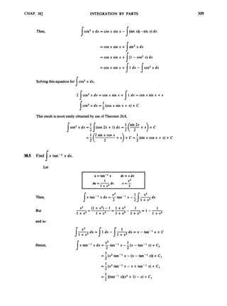
![310
3
8
.
6
38.7
38.8
38.9
38.10
38.11
38.12
38.13
Compute:
(a) dx
(e) I x cos x dx
(i) Ieaxcos bx dx
(m) dx
(4) I x sin 2x dx
(U) I x 2 tan-' x dx
INTEGRATION BY PARTS
Supplementary Problems
(b) I e x sin x dx
(f) I x 2 sin x dx
0
9 I s i n ' x d x
(n) {xse!c2 x dx
(r) { x sin x2 dx
(U) 11. (x2 + 1)dx
(c) s x 3 e xdx
(g) 1.0.(In x ) dx
(k) 1 ~ 0 s '
x dx
(0) I x cos2x dx
(s) {%dx
[CHAP. 38
(d) [ s i n - ' x d x
J
P
(h) Ix cos (5x - 1)dx
J
*
J
fl
[Hint: Integration by parts is not a good method for part (r).]
Let 41 be the region bounded by the curve y = In x, the x-axis, and the line x = e. (a) Find the area of 41.
(b) Find the volume generated by revolvingW about (i)the x-axis;(ii) the y-axis.
Let 9 be the region bounded by the curve y = x-' In x, the x-axis, and the line x = e. Find: (a)the area
of 9;(b) the volume of the solid generated by revolving 41 about the y-axis; (c) the volume of the solid
generated by revolvingW about the x-axis. [Hint:
In part (c), the volume integral,let U = (In x ) ~ ,
Y = -l/x,
and use Problem 38.6(s).]
Derive from Problem 38.8(c)the (good)bounds: 2.5 s e I; 2.823. [Hint: By Problem 30.3(c),
5 e - 1
0 I; 2 - - 5 -
or
0I; [(yydx I; 5
e2 e e2
The left-hand inequality gives e 2 3;the right-hand inequalitygives e 5 (3 +&2.]
Let 9t be the region under one arch of the curve y = sin x, above the x-axis, and between x = 0 and x = n.
Find the volume of the solid generated by revolving9 about: (a)the x-axis;(b) the y-axis.
If n is a positive integer,find:
(a) I x x cos nx dx (b) J'bx sin nx dx
For n = 2, 3,4, ...,find reduction formulasfor:
(a) !cos" x dx
(c)Use these formulasto check the answers to Problems 38.4,38.6(k), 38.6(1),and 38.60).
(b) Isin" x dx
(a) Find a reduction formula for I sec" x dx (n = 2, 3, 4, ...). (b) Use this formula, together with Problem
34.7, to compute: (i)I sec3x dx; (ii) sec4 x dx.](https://image.slidesharecdn.com/problemscalculus-221128025033-038ef06f/85/problems-calculus-pdf-323-320.jpg)
![CHAP. 391 TRIGONOMETRIC INTEGRANDS AND TRIGONOMETRIC SUBSTITUTIONS 313
Similarly,from
sec x dx =In lsec x +tan xl +C
I
and the reduction formulaof Problem 38.13(a), we can integrate all powers of sec x.
Antiderivatives of the forms
using the identities
sin Ax cos Bx dx, 5 sin Ax sin Bx dx, cos Ax cos Bx dx can be computed by
1
2
1
2
1
2
sin Ax cos Bx = - (sin (A +B)x +sin (A -B)x)
sin Ax sin Bx = - (cos (A -B)x - cos (A +B)x)
cos Ax cos Bx = - (cos (A -B)x +cos (A +B)x)
For instance,
11
sin 8x sin 3x dx = - (cos 5x - cos 1lx) dx =-
s I:
39.2 TRIGONOMETRIC SUBSTITUTIONS
,
/
=
,
it is often helpful to substitute a trigonometric function for x.
To find the antiderivative of a function involving such expressions as ,
/
-
’ or ,
/
G
2
or
EXAMPLES
(a) Evaluate ,
/
- dx.
I
None of the methods already available is of any use here. Let us make the substitution x = fi tan 8,
where -n/2 -c8 < n/2. Equivalently, 8= tan-’ (x/&). Figure 39-1 illustrates the relationship between x
and 8,with 8interpreted as an angle. We have dx = fi sec’ 8d8 and, from Fig. 39-1,
--
m - e c e or , / ~ = a = e
a
where sec 8> 0 (since -n/2 < 8 -cn/2).Thus,
Id mdx = I($ sec 8 X f i sec2 8)d8 = 2
= sec 8 tan 8 +In lsec 8 +tan 81+C [by Problem 38.13(b)]
J2 J2 I J2 J2l
Note how the constant -In was absorbed in the constant term in the last step. The absolutevalue signs in
the logarithm may be dropped, since Jm
+x > 0 for all x. This follows from the fact that d m>
p=
1x1 2 -x.
This example illustrates the following general rule: If ,
/
G
2
occurs in an integrand, try the
substitution x = U tan 8 with -(n/2) < 8 -=(42).](https://image.slidesharecdn.com/problemscalculus-221128025033-038ef06f/85/problems-calculus-pdf-326-320.jpg)
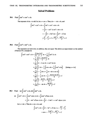
![316 TRIGONOMETRIC INTEGRANDS AND TRIGONOMETRIC SUBSTITUTIONS [CHAP. 39
(b) This antiderivative was essentiallyobtained in Problem 39.2,
sin4 x dx = 2 sin4 (2u)du
pet u = i]
I I sin 8u
= 2 -16
(3u -sin 4
u +-
sin 4x
= f (F-sin 2x +-
8
128 8
>,,
39.4 Find tan' x dx.
s
From the reduction formula (39.2),
tan2 x
tan x dx = -- In Isec x I
I 2 I 2
tan2 x
tan3 x dx = --
tan4 x tan2 x
tan3 x dx = -- -+In lsec x l +C
I 4 I 4 2
tan4 x
tan' x dx = -
-
39.5 Show how to find { tanPx secqx dx: (a) when 4 is even; (6) when p is odd. (c) Illustrate both
techniques with 1tan3 x sec4x dx and show that the two answers are equivalent.
(a) Let q = 2r (r = 1,2,3, ...).Then
a a
J J
a
= J tanp x ( l + tan2 xy-l(sec2 x) dx
since 1 +tan2 x = sec2 x. Now the substitution u = tan x, du = sec2x dx, produces a polynomial
integrand.
(b) Let p = 2s + 1(s = 0, 1, 2,. ..). Then,
tan2s+'x sec4 x dx = tan2' x secq- x(sec x tan x) dx
I
s
= J' (sec2 x - ly sec4- 1 x(sec x tan x) dx
I
I
since tan2 x = sec2x - 1.Now let U = sec x, du = sec x tan x dx, to obtain a polynomial integrand.
(4 BY Part (4
tan3 x sec4x dx = tan3 x(1 +tan2 x)(sec2 x) dx
= 1u3(1 +u2) du = I ( u 3 + du
u4 u6 tan4 x tan6 x
4 6 4 6
=-+-+c=-+- + C
tan3 x sec4 x dx = !(sec2 x - 1) sec3 x(sec x tan x) dx
= [(U. - l)u3 du = (us - u3) du
+ C
u6 u4 sec6 x sec4 x
= - - - + c = - - -
6 4 6 4
I
I](https://image.slidesharecdn.com/problemscalculus-221128025033-038ef06f/85/problems-calculus-pdf-329-320.jpg)
![CHAP. 391 TRIGONOMETRIC INTEGRANDS AND TRIGONOMETRIC SUBSTITUTIONS 317
Since 1 +u2 = u2,
u6 u4 4u6- 6u4 4(1 +u ~ ) ~
-6(1 +u ~ ) ~
-
-
-_-- -
6 4 24 24
ALGEBRA (1 +t)3 = 1 +3t +3t2 +t3
q1 +3u2 +3u4 +u6) - q1 +2u2+u4)
-
24
4 + 12u2+ 12u4+4u6 -6 - 12u2- 6u4
-
24
6u4 +4u6 - 2 u4 u6 1
-
- =-+---
24 4 6 12
and so the two expressions for tan3 x sec4 x dx are equivalent. (The -Ais soaked up by the arbi-
trary constant C.)
39.6 Find tan' x sec x dx.
s
Problem 39.5 is of no help here.
tan2 x sec x dx = (sec2x - 1) sec x dx = (sec3x - sec x) dx
I s I
1
2
1 1
2 2
= - (sec x tan x +In Isec x +tan x I)- In Isec x +tan x I+ C
=-sec x tan x --In /secx +tan xl +C
[by Problem 38.13(b)]
39.7 Prove the trigonometric identity sin Ax cos Bx = *(sin (A +B)x +sin (A - B)x).
The sum and differenceformulas of Theorem 26.6give
sin ( A +B)x = sin (Ax +Bx) = sin Ax cos Bx +cos Ax sin Bx
sin ( A - B)x = sin (Ax - Bx) = sin Ax cos Bx -cos Ax sin Bx
and so, by addition, sin ( A +B)x +sin ( A - B)x = 2 sin Ax cos Bx.
39.8 Compute the value of sin nx cos kx dx for positive integers n and k.
1
'
Case I : n # k. By Problem 39.7, with A = n and B = k,
Jr:^sin nx cos kx dx = - [=(sin (n +k)x +sin (n - k)x)dx
2 n + k 0
1 cos (n +k)x + cos; ,t*>12*
--( - = O
because cos px is, for p an integer, a periodic function of period 2n.
Case 2: n = k. Then, by the double-angle formula for the sine function,
1 cos 2nx 2*
sin nx cos nx dx =- sin 2nx dx = -5(
T
)
]
= 0
r ;](https://image.slidesharecdn.com/problemscalculus-221128025033-038ef06f/85/problems-calculus-pdf-330-320.jpg)
![318 TRIGONOMETRIC INTEGRANDS AND TRIGONOMETRIC SUBSTITUTIONS [CHAP. 39
dx
J;m*
39.9 Find
The presenceof ,
/
- suggestsletting x = 3 tan 8. Then dx = 3 sec28 do, and
,
/
=
= ,
/
- = J
- = 3 , / S = 3 sec 8
NOTE
and the constant -In 3 can be absorbed in the arbitrary constant K.Furthermore,
Jm-
+x > 0
dx
39.10 Find
and
The presenceof ,
/
- suggeststhe substitution x = J?sin 8.Then, dx = J?cos 8 do.
,
/
=
= ,/KG23 = J
- = & J c X = JScos e
dx
1
3
= - - c o t e + c
But
Hence,
dx
3x
39.11 Find
The occurrenceof ,
/
- suggeststhe substitutionx = 2 sec 8. Then dx = 2 sec 8 tan 8 do.
JZ'=
JGZiFi = ,
/
- = 2,/- = 2 tan e
d8 = 4 sec38 d8
5
X2 sec28x2 sec 8 tan 8)
and 1- dx = 5'" 2 tan 8
= 2(sec 8 tan 8 +In Isec 8 +tan 81) +C [by Problem 38.13(b)]
+ C
-
- xF-
x - 4 + 2 In Ix +J
=
2 2
+2 In ~x+,/Z
- xJx2 -4
-
2
where K = C - 2 In 2 (compareProblem 39.9).
+ C
+ K](https://image.slidesharecdn.com/problemscalculus-221128025033-038ef06f/85/problems-calculus-pdf-331-320.jpg)
![CHAP. 391 TRIGONOMETRIC INTEGRANDS AND TRIGONOMETRIC SUBSTITUTIONS 319
SupplementaryProblems
39.12 Find the followingantiderivatives:
(a) J'sin x cos2 x dx (b) !cos2 3x dx (c) ]sin4 x cos' x dx (d) [cos6 x dx
(e) x sin2x dx (f) J'tan2 5dx (g) J'tan6 x dx (h) [sec' x dx
(i) [tan2 x sec4 x dx
(m) Isin nx cos 3nx dx
6
9 [tan3 x sec3x dx
(n) J'sin 5x sin 7x dx
(k) [tan4 x sec x dx
(0) l c o s 4x cos 9x dx
(0 [sin 2x cos 2x dx
39.13
39.14
39.15
39.16
39.17
39.18
39.19
Prove the followingidentities:
1
2
1
2
(a) sin Ax sin Bx = -(cos (A -B)x -cos (A +B)x)
(b) COS Ax COS Bx =- (COS (A -B)x +COS (A +B)x)
Calculate the followingdefiniteintegrals,where the positive integers n and k are distinct:
(a) sin nx sin kx dx (b) 1%
sin2nx dx
0
Evaluate:
dx
(i) [ x 2 , / E i d x 0
9 [ e 3 x , / s dx
(k) I(x' - 6x + 13)2
[Hint: In part (k),completethe square.]
Find the arc length of the parabola y = x2from (0,O) to (2,4).
Find the arc length of the curve y = In x from(1,O) to (e, 1).
Find the arc length of the curve y = 8 from (0, 1)to (1,e).
Find the arc length of the curve y = In cos x from (0,O) to (n/3, -In 2).
39.20
x2 y2
Find the a
r
e
a enclosed by the ellipse-+-= 1.
9 4](https://image.slidesharecdn.com/problemscalculus-221128025033-038ef06f/85/problems-calculus-pdf-332-320.jpg)
![Chapter 40
Integration of Rational Functions;
The Methodof Partial Fractions
This chapter w
i
l
lgive a general method for evaluating indefinite integrals of the type
where N(x)and D(x)are polynomials. That is to say, we shall show how to find the antiderivative of any
rational functionf(x) = N(x)/D(x)(see Section 9.3). Two assumptions will be made, neither of which is
really restrictive: (i) the leading coeficient (the coefficient of the highest power of x) in D(x) is +l;
(ii)N(x)is of lower degree than D(x)[that is,j'(x) is a proper rational function].
EXAMPLES
(a) - 4 ~ ' ~
+3x - 11
(b) Considerthe improper rationalfunctionf(x) = -
.Long division(see Fig.40-1) yields
-56x4
-
-
-7 8x4
-7 -jx'O + 3x - 11
--
-
8x4
x10 - 2 1 ~
+77
x4 +7x
x2 - 1
7x + 1
f(x) = x2 + 1 +-
x2 - 1
Consequently,
I f ( x ) dx = 1 ( x 2 + 1) dx +I-7x + 1 dx = -+
x3 x + 7x + 1
x2 - 1 3
and the problem reduces to finding the antiderivativeof a proper rational function.
x 2 + 1
x2 - 1 I x4 + 7x
x4 - x2
x2 + 7x
x2 - 1
7x + 1
Fig. 40-1
The theorems that follow hold for polynomials with arbitrary real coefficients. However, for sim-
plicity we shall illustrate them only with polynomials whose coefficientsare integers.
Theorem 40.1: Any polynomial D(x) with leading coefficient 1 can be expressed as the product of
linearfactors, of the form x - a, and irreducible quadraticfactors (that cannot be fac-
tored further),of the form x2 +bx +c, repetition of factors being allowed.
As explained in Section 7.4, the real roots of D(x)determineits linear factors.
320](https://image.slidesharecdn.com/problemscalculus-221128025033-038ef06f/85/problems-calculus-pdf-333-320.jpg)
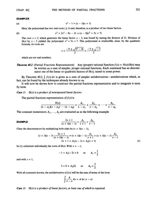
![322 THE METHOD OF PARTIAL FRACTIONS [CHAP. 40
This is treated in the same manner as in Case 1,except that a repeated factor (x - a)’ gives rise to a
sum of the form
A2 A&
x - a ( x - a ) (x -
+
y
+* * * +-
A1
EXAMPLE A2 A3
+-+-
A ,
(x - 1)2(x -2) x - 1 (x - 1)2 x -2
=-
3x + 1
Multiply by (x - 1)’(x - 2),
3x + 1 = A,(x - 1)(x - 2) +A,(x -
Letting x = 1,
4 = O + A 2 ( - 1 ) + 0 or
Letting x = 2,
7 = 0 +0 +A3(l) or
The remaining numerator, A,, is determined by the condition thal
zero (sinceit is zeroon the left side). Thus,
2) +A,(x - 1)2
A2 = -4
A, = 7
the coefficient of x2 on the right side of (2) be
A , +A3 =0 or A , = -A3 = -7
[More generally, we u
s
e all the roots of D(x) to determine some of the A’s, and then compare coefficients-of as
many powers of x as necessary-to find the remainingA’s.]
Now the antiderivatives off (x) will consist of terms of the form In Ix - a Iplus at least one term of
the form
C a e 3: D(x)has irreduciblequadraticfactors, but none is repeated.
In this case, each quadratic factor x2 +bx +c contributes a term
A x + B
x2 +bx +c
to the partial fractions representation.
EXAMPLE
Multiply by (x2 + 1)(x +2),
-t
x2 - 1 A1
=-
(x2 + 1)(x +2) x +2
x2 - 1 = A1(x2 + 1) +( A ~ x
+A3Xx +2)
Letx= -2,
3
3 = Al(5) +O or A, = -
5
Comparingcoefficients of xo(theconstant terms),
1 4
- 1 = A , + 2 A 3 or A , = - - ( ~ + A , ) = - -
2 5
Comparing coefficientsof x2,
CI
1 = A , + A 2 or A 2 = 1 - A , = 4
5](https://image.slidesharecdn.com/problemscalculus-221128025033-038ef06f/85/problems-calculus-pdf-335-320.jpg)
![CHAP. 4Q] THE METHOD OF PARTIAL FRACTIONS 325
1
Let x = -3, 9 = 0 +0 +A3(-6)2 or A, = 4
Compare coefficientsof x2,
3
l =A ,+A , or A,=l-A,=-
4
Thus,
and
3 1 3 1 1 1
=-- +--+--
x3-3x2-9x+27 4 ~ - 3 2 ( ~ - 3 ) ~4 ~ + 3
X2
x2 dx 3 3 1 1
2 x - 3 4
= - In I x - 31 - - -+- In I x + 31 +C
Ix3 - 3x2- 9~ +27 4
4
0
.
3 F i n d 1 dx.
x(x2 +2)
This is Case 3,
x + l A , A , x + A ,
-=-+
x(x2 +2) x x2 +2
Multiply by x(x2 +2),
x + 1 = A,(x’ +2) +x(A,x +A,)
Letx=o,
Compare coefficients of x2,
1
1 =2A, + O or A, = -
2
1
O = A , + A 2 or A , = - A , = - -
2
Compare coefficientsof x,
1=A,
Thus,
and
-
x + l = 1(A) + (-4). +-1
x(x2 +2) 2 x x2 +2
Because the quadratic factor x2 +2 is a complete square, we can perform the integrations on the right
without a change of variable,
x + l 1 1 X
1x1--In (x2+2) +-tan-’ -+C
4 & f i
P .
1
dx.
J 1- sin x +cos x
40.4 Evaluate
Observe that the integrand is a rationalfunction a. sin x and cos x. Any rational function c. the six
trigonometric functions reduces to a function of this type, and the method we shall use to solve this
particular problem will work for any such function.
Make the change of variable z = tan (x/2); that is, x = 2 tan- z. Then,
dx = -
dz
1 + z 2](https://image.slidesharecdn.com/problemscalculus-221128025033-038ef06f/85/problems-calculus-pdf-338-320.jpg)
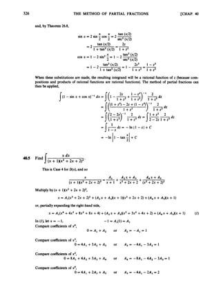
![CHAP. 403 THE METHOD OF PARTIAL FRACTIONS 327
Therefore,
x dx dx (x + 1)dx (x +2) dx
/(x + 1)(x2+2x +2)2= -1 + Jx2 +2x +2 + J(x2 +2x +2)2
U du U du du
[by quick formulas I1 and I]
= -InIx+II+-ln(u2+1)--
1 '(-
)+Jms2ede
2 2 u 2 + 1
[Case 4: let U = tan 01
1 1 8 sin 28
2
= --InIx+ ll+-In(x2+2x+2)-- + C
Now
and (see Problem 40.4)
8 = tan-' U = tan-' (x + 1)
2 tan 9 - 2(x+ 1)
1+tan28 - x2+2x +2
sin 28 =
so that we have, finally,
x dx 1
2
= -lnIx+ ll+-1n(x2+2x+2)--
J(x + lXX2 +2x +2)2
+-
1tan-' (x + 1) +-
1( x + l ) + c
2 2 x2+2x+2
X
=1(In (x2 +2x +2) + +tan-' (x + 1)) - In Ix + 1I +c
2 x2+2x +2
SupplementaryProblems
40.6 Find the followingantiderivatives:
x dx
x2- 9
2x2+ 1 x2- 4
x dx x - 5
dx
(
' /(x - 1Xx - 2)(x - 3)
(
'
) /x4 - 13x2+36
x4 dx
x2dx dx
(n)
(
'
) I ( x - l)(x2 +4)2
+ 1xx2+4)
x2dx
x - 1 x2+2
dx
/x(x2 +5x +6)
dx
x3 +2x2-x - 2
(c) 5"-4x2+x + 1
I-
dx
x2 -4
x3+ 1
dx
(f) Jx(x +3Kx +2)(x - 1)
(i) J( 2x dx
x - 2)2(x +2)
dx
x4 + 1
(r)
x3 +
dx
x(x2+x +1)2](https://image.slidesharecdn.com/problemscalculus-221128025033-038ef06f/85/problems-calculus-pdf-340-320.jpg)
![328 THE METHOD OF PARTIAL FRACTIONS [CHAP. 40
40.7 Show that p(x) = x2 +bx +c is irreducible if and only if c -(b2/4)
> 0
.[Hint: A quadratic polynomial is
irreducibleif and only if it has no linear factor; that is (byTheorem 7.2),if and only if it has no real root.]
4
0
.
8 (a) Find the area of the region in the first quadrant under the curve y = l/(x3 +27) and to the left of the
line x = 3.
(b) Find the volume of the solid generated by revolving the region of part (a)around the y-axis.
dx
1 -sin x
4
0
.
9 Find I
- . [Hint: See Problem 4
0
.
4
.
1
cos x dx
sin x - 1*
answers are equivalent.
40.10 Find 1
- (a) Use the method of Problem 40.4.(b) Use the quick formula 11. (c) Verify that your
40.11 Evaluate the followingintegralsinvolvingfractionalpowers:
[Hints: Part (a)let x = z3;part (b)let x - 1 = z4; part (c) let 1 +3x = z2; part (d)let x = P
.
3](https://image.slidesharecdn.com/problemscalculus-221128025033-038ef06f/85/problems-calculus-pdf-341-320.jpg)
![Appendix B
Basic Integration Formulas
a d x = a x + C
s
X
tan-' - +C
a2 + x 2 a a
dx 1 X
a
--sec-'-+C [a>O]
ex dx = e" +C
s
xe" dx = eyx - 1) +c
In x dx = x In x - x +C
s
s
s
s
sinxdx= - c o s x + C
cos x dx = sin x +C
tan x dx =In lsec x l +C
sec x dx = In /sec x +tan xl +C
cot x dx =In (sinxl +C
s
s
s
s
s
s
s
s
csc x dx = In lcsc x - cot xl +C
sec2 x dx = tan x + C
csc2 x dx = -cot x + c
sec x tan x dx = sec x +C
csc x cot x dx = -csc x +c
x sin 2x
2 4
x sin 2x
sin2x dx = - --+ C
cos2 x dx = - +-+ C
s
s 2 4
tan2 x dx = tan x - x +C
s
330](https://image.slidesharecdn.com/problemscalculus-221128025033-038ef06f/85/problems-calculus-pdf-343-320.jpg)
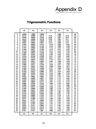
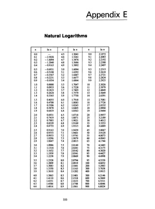
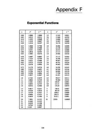
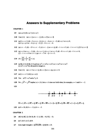
![336 ANSWERS. TO SUPPLEMENTARY PROBLEMS
0
c
/
//
0
/
/
2.8 (3,4). 2
.
9 (- 1, 1) and (3,O). 2.10 (0,2),(6,2),(4, -4).
2.11 (2,y)for some real numbery.
0
’
0
0
/
/
*0
-X
J389
2.12 (a)p 4 ; (b)3Jz; (c) .
2.13 (a)Isoscelesonly; (b)right only, area = 10;(c)isoscelesright, area = 17.
2.14 k = 5. 2.15 (a)No; (b)yes.
2.16 (4(4, 2);(b)(i,
2); (4(
7
,
2).
5 + $
2-17 (5,8).
CHAPTER 3
3.9 See Fig. A-1.
( h )
Fig. A-1
3~10 See Fig. A-2. 3.11 SeeFig. A-3. 3.12 See Fig. A-4. 3.13 x2 = 4py (parabola).
3.14 (U) (X -4)2+0) - 3)2 = 1; (b)( X + +0) - 5)2 2;(c)x2 +(U - 2)2= 16;(a)( X - 3)2 +0) - 3)2 = 18;
(e) (x -412+(y + 112= 20; (f)
(x - +0) -2J2= 5.
3.15 (a)Circle [center (6, -lO), radius 1I]; (b)circle [center (0, -15), radius 141;(c)null set;
(a)circle [center (a,0),radius 41;(e) point (- 1, 1); (f)
circle [center (-3, -2), radius 7).](https://image.slidesharecdn.com/problemscalculus-221128025033-038ef06f/85/problems-calculus-pdf-349-320.jpg)
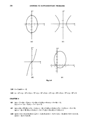
![ANSWERS TO SUPPLEMEWARY PROBLEMS 339
4.11 k -9. 4.12 NO.
4.13 (a)Yes; (c) in all cua;
(a)k = -4.
414 (a] Yvrlkl:(h)&her; (c)paralkl;(d)perpendimtar;(c) neither.
115 (a)y -fx +32;(h) -40".
116 (a)10; (6) -15; (c) -f ;(d)9.
117 ( 4 y = -+X +#;(b)y - 4 ~
+3 2 : ( ~ ) p
;
X -4.
118 (12.9) is not an the linc;(d, 3)is on tbc line.
4
.
2
2 4x +3y -9 >Oondx > I;= F
i
g A-5.
4
.
2
3 x<200/3. 4J4 SacFig.A-6.
166 (U) AN nonvcrtid lines throughtbe point (0.2); (b)all Lineswith slope3.
4.27 (4Horizmlal lina;(b)(4
2; (194; (If04;(h13; (n)none.
a (a)y- -$x +3 ; ( b ) ~ -- X +9 ; ( ~ ) y m 4 ~ + # .
f'](https://image.slidesharecdn.com/problemscalculus-221128025033-038ef06f/85/problems-calculus-pdf-352-320.jpg)
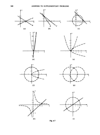
![ANSWERS TO SUPPLEMENTARY PROBLEMS
CHAPTER 5
341
(i) (Aa,
Af i )
and (-Afi,- @);(j)null set. See Fig. A-7.
8
5.6 (b)5fi z 3.58. 5.7 x = 50. 5.8 Center
4
5.9 x = 0and y = -- X. 5.10 (33/2,34).
3
CHAPTER 6
6.6 (a)y-axis; (b)origin; (c)x-axis, y-axis,origin; (d)x-axis, y-axis, origin; (e)x-axis; (f) none;
(9)origin; (h) none; (i) y-axis;(j)y-axis;(k) origin; (0none.
6.7 (a)x2 +xy +y2 = 1;(b) y3 +xy2 -x3 = 8; (c)x2 + 12x - 3y = 1;(d) y = -3x + 1; (e) no change.
CHAPTER 7
7.8 (Let R denote the set of real numbers. In each answer, the first set is the domain, the second set the
range. The graphs are sketched in Fig. A-8.) (a)R, (- a,41; (b) CO,a
)
,
(- a , O ] ; (c) [-2,2], range of H
is CO,21, range of J is [-2,Ol; (d)
(- a,-21 U [2, a)
(union or “sum” of the two intervals),CO, a
)
;
(e)R, CO,a
)
;
(f) R, set of all integers;(9)R, set of all integers; (h) R - (0) (set of all real numbers except 0),
R - (0);
(0R - {I},R - (0);
U)R, R;(4
R, R;(0R,c2, 4;(m)
(1,2,4), { -43); (4
R -{--2}, R - { -4};
(0) R, (-a,
21 U (4); (PI R - (O), {-1, 1);(4)
R, c2, 4;(r)R, R; (4R, CO, 1); (t)R,R.
7.10 (c)and (d).
2 x - 1
x3’ x + l
7.11 (a)f(x) = - domain is R - (0); (b)f(x) = -
,domain is R - { -1);(c)f(x) = x, domain is R.
7.12 (a) Domain is R - (2, 3}, range is (0,00) U (- a,-41; (b) (- 1, l),(1, a
)
;
(c)(- 1, a
)
,
(0,2];
(4CO,4), c- 1921;(4R, CO, 4.
7.13 (a) k = -8; (b)fis not defined when x = 0, but g is.
7.14 Of the infinitely many correct answers, some examples are: (a)f(x) = 2x for 0 < x < 1;
(b)f(x) = 5x - 1for 0 Ix < 1;(c)f(x) =
0 ifx=O
1 ifx>O’* (d)f(x) = (x - + 1for x < 1 or 1 < x < 2.
7.15 (U) y-axis; (b) none; (c)y-axis for both; (d) y-axis; (e) none; (f)
none; (g) none; (h)origin; (4 none;
( j )origin; (k) origin; (0none; (m) none; (n)none; (0)
none; (p) origin; (4)
none; (r)none; (s) none;
(t) origin.
7.16 (a)Even; (b) neither; (c) both even; (d) even; (e)neither; (f) neither; (g) neither; (h)odd; (i) neither;
(
1
1odd; (k) odd; (I) neither; (m) neither; (n)neither; (0)
neither; Cp) odd; (4)
neither; (r)neither;
(s) neither; (t) odd.
7.17 (a)No; (b) yes; (c) k = 0;(d) k = 2; (e)yes;f(x) = 0for all x.](https://image.slidesharecdn.com/problemscalculus-221128025033-038ef06f/85/problems-calculus-pdf-354-320.jpg)
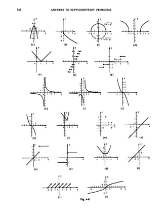
![ANSWERS TO SUPPLEMENTARY PROBLEMS 343
7.18
7.19
7.20
7.24
7.25
1 1 Ix +h l - 1x1
- 5 ; w h
JxT-i;+&;(e)J Z i +J;
(U) 2x +h - 2; (b) 1;(c) 3x2+3hx +h2;(d)
(U) 1, -1,3, -3; (b) -2,4, -4; (c)2, -2,3; (42; (e) -2, -3, -4; (f)-2, 1+fi,1 - fi;
(B)4,49 -fi.
One, two (oneof them repeated),or three. 7.21 (a) k = 3; (b) k = -2. 7.22 9 and -12. 7.23 (iii).
(a)x< - 2 o r x > l;(b) - 2 < x < O o r x > 1.
CHAPTER 8
(c)lim 7 = 7;
(f)
lim (1Ox +5h - 2) = 1Ox - 2.
1
1
- -
-
'
-1
8.6 (a) lim (6x +3h) = 6x; (b) lim
(d) lim (3x2+3xh +h2)= 3x2;(e)lim
h+O h+O (X +h + 1)(X+1)- (X + h+O
=-.
1
h-rO h-0 J F i +& 2&' h+O
8.9 (4. 8.10 (a) lim (x3+x2 +x + 1)= 4. 8.11 (a) &. 8.12 (a) 0; (b) A;(c)8;(d) no limit.
x+ 1
CHAPTER 9
9.6
9.7
9.8
9.9
9.11
(a)12andll;(b)land -l;(c) -oo;(d) +wand -co;(e)landl;(f) -wand +m;(g)OandO;
(h)3 and 3;(i) +00 and -00; (I]0 and 0; (k)4 and -4; (Z) +00 and -00; (m)0 and undefined
(denominatorundefined when x3 < -5);(n)0 and 0; (0)2 and 2; (p) +00 and -00 ;(4)-3;(r) +00;
(s) +0O.
(a)No asymptotes;(b) vertical asymptote:x = -3; horizontalasymptote: y = 3(to the left and the right);
(c)vertical asymptotes:x = -3, x = 2; horizontal asymptote:y = 0 (to the left and the right);
(a)vertical asymptotes: x = -4, x = 1;horizontal asymptote:y = 0 (to the left and the right);
(e) vertical asymptotes: x = -2; horizontal asymptote:y = 0(to the left and the right);
(f)
vertical asymptotes:x = -4, x = 2; horizontal asymptotes:y = 1(to the right)and y = -1(to the left);
(8)horizontal asymptotes:y = 2 (to the right)and y = -2 (to the left);(h)horizontal asymptote:y = 0 (to
the right);(i) horizontal asymptote:y =0 (to the right).
(a) Vertical asymptote: x = 4; horizontal asymptote:y = -3; (b)vertical asymptote:x = 4; horizontal
asymptotes:y = -1(to the right) and y = 1(to the left);(c) horizontalasymptotes:y = -1(to the right),
y = 1(to the left);(4horizontal asymptote:y = 0 (to the right);(e)horizontal asymptote:y = 2.
CHAPTER 10
10.6 (a) Continuouseverywhere;(b) continuous for x # 0;(c)continuouseverywhere;
(6)continuousfor x # -2; (e)continuouseverywhere;(f)
continuousexcept at x = 1 and x = 2.](https://image.slidesharecdn.com/problemscalculus-221128025033-038ef06f/85/problems-calculus-pdf-356-320.jpg)
![344 ANSWERS TO SUPPLEMENTARY PROBLEMS
10.7 (a) Continuouson the right but not on the left at x = 0; (b) discontinuous on both the left and the right at
any nonnegativeintegerx; (c) no points of discontinuity;(6)continuouson the left but not on the right at
x = -3andatx=2.
1 i f x r o
O ifx<O'
0 i f - 2 r ; x < - 1
0 if 1 < x < 2
10.9 (a) Yes; (b)-(d)no; (e) Problem lO.?)--none, Problem 10.4-no.
10.10 (a) x = 4, x = -1;(b) lim f ( x )does not exist, lim f ( x )= -3;
(c) x = 4 (verticalasymptote),y = 0(horizontalasymptote).
x+4 x + - 1
10.11 (a) x = 0;(b)x = 0 (verticalasymptote),no horizontal asymptote.
10.12 (a) No; (b) no; (c) yes; (d)no. 10.13 c = 8.
10.14 (a) Yes; (b)yes; (c) no. 10.15 (b) 6. 10.16 Discontinuousfor all x.
CHAPTER 11
11.6
11.7
11.10
(a) (i)slope = 4x + 1;(ii)y = 2x - 6;(iii) see Fig. A-9(a); (b)(i)slope = x2;(ii)y = 4x - 9,
(iii)see Fig. A-9(b); (c) (i)slope = 2x - 2; (ii) y = -1;(iii)see Fig. A-9(c); (6)(i)slope = 8x; (ii)y = 4x +2;
(iii)see Fig. A-qd).
28
27
(3,9). 11.8 (1, 1)and (- 1, -1). 11.9 y = -3x +-
1 55 1
4
(3, 5) and (-j,7)
. 11.12 (6, 36) and (-2,4). 11.13 y = -x + 1.
CHAPTER 12
126
127
128
129
12.10
1211
1213
1214
(a) 9x2 - 8x + 5 ; (b) -40x4 +3 8 x 2 +4nx; (c) 3 9 ~ ' ~
- 50x9 +20x; (d)lO2XS0 +36x" - 28x +fi.
(a) 21x6-x4; (b) 6x - 5; (c) 2x3+5; (d)21t6 -24t; (e) 5 8 x 4 - 3x2.
(u)Y= -7x+ l;(b)y=66x- 1 5 3 ; ( ~ ) ~ = 3 .
85 65
(a)y = 20x +2andy = -44x +2;(b)y = x +4andy =- x - -
4 4 '
y = --x + 1. 1212 (2,2).
20
(a) ox(xS)
IX=j = 405; (b)0,t(5x4)I x t 113 = 27-
f'(x) = 8x [(iii) givesf'(u) = ku;then choose U = U = 1in (iii)].](https://image.slidesharecdn.com/problemscalculus-221128025033-038ef06f/85/problems-calculus-pdf-357-320.jpg)
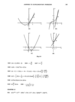
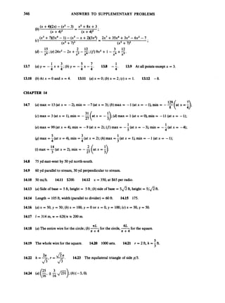
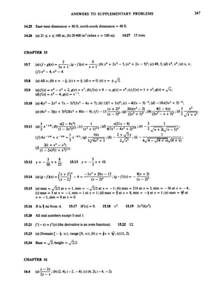
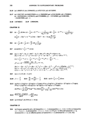
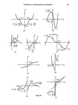
![352 ANSWERS TO SUPPLEMENTARY PROBLEMS
23.5 (a) 1.5(min);(b)0 (max),3 (min), -3 (min);(c)4 (min), -4 (max);(d)0 (max),2 (min);(e)0 (min).
23.6 SeeFig. A-10. 23.7 (a). 23.8 Band E.
23.9 (a)One;(b)none; (c)parabola. 23.10 (f). 23.11 -4 < k < 0
. 23.12 See Fig. A-11.
23.13 (a)Allx in [-1,2]; @)allx in [-1,2] but x = 1 [f'(x) = 2x - 1 for x > 1, andf'(x) = 1 - 2x for x < 1);
(c) 1 < x < 2 or -1 < x < 4; (d)f"(x)= 2 for x > 1, andf"(x) = -2 for x < 1;(e)concaveupward for
x > 1, concavedownwardfor x < 1; (I)
see Fig. A-12.
23.15 k = -4. 23.16 A = C = 0
,D = 1, B = -4, k = -+d.
t' t'
I I'
-'I
X
Fig. A-11](https://image.slidesharecdn.com/problemscalculus-221128025033-038ef06f/85/problems-calculus-pdf-365-320.jpg)
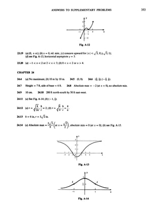
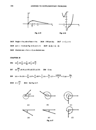
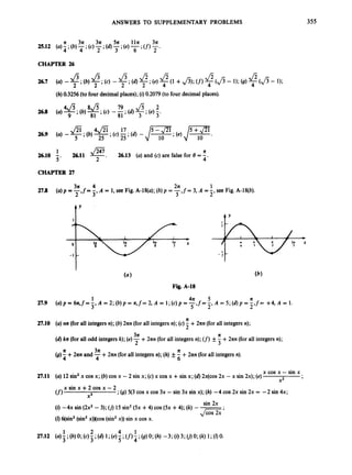
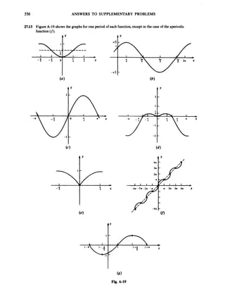
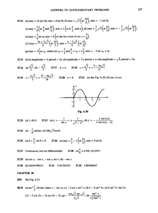
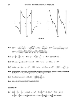
![ANSWERS TO SUPPLEMENTARY PROBLEMS 359
6 4 2
3 15
(h);
x512 -- X3/2 + 2x112 +C = -&9x2 - 1Ox + 15) +C;(i)
-3 cos x +5 sin x +C;
1 2
10 3
(m) sin x +C; (n)tan x -x +C;(0)-x10 +- x6 +2x2+C.
2 1 1
21 39 3
298 (a)-(7x +4)3/2+c;(b)2(x - 1p2+c;(c) -(3x - 5)13 +c;(6)- -cos (3x - 1) +c;
(e) 2 tan - +C; (f)
2 sin J;;+C;(g) --(4 - 22)' +C;(h)i(x3 + 5)4/3 +C;
X 1 1
2 32
2 2 3
3 3 5
3 1 1 3 1
(i) -(x + 11312- 2 ( ~
+ iy2
+c = - ,/iTT(x -2) +c;( j )-(x - 1)5/3+ c;
(k) [?
(x4 + 1)7/3
-- (x4 + 1)4/3] +c= (x4 + 1)4/3(4~4
- 3) +C;(0 Js
+C;
4
2(ax +b)3/2 1 1
+ c =--csc3x+c;
(3ax - 2b) +C;(n)- -
(m) 15a2 3 sin 3x
(0) -2(1 - x)~/~[-
-- (1 -x) + (1 - x)I] +C = - -(1 -x)312(15~2
+ 12x +8) +C;
3
1 2 1 2
3 5 105
1 1 1 1 1 3
112 2 x 12 x4
(p)5(3x - 5)13 +c;(4)--(4 - 7t2)' +C;(r) -- sin2- +C;(s) --tan -+ C.
29.9 (a) t = 7 sec;(b)1024ft;(c) t = 15 sec;(6) 256 ft/sec.
40 35
+4t;(c)at x = -when t = 4,at x = --when t = -1;
3 6
t3 3t2
(U) U = t2 -3t +4; (b)x =-- -
3 2
(6) -1 < t <4.
29.10
t4 13t2 23 3
12 4
12 6
+4t; (c)at x =-when t = 1, at x = - -when t = 3, and at
t +4; (b)x = -- -
t3 13
29.11 (a) U = ---
3 3
when t = -4; (6)t < -4 and 1 < t < 3.
88
3
X = - -
29.12 (a) 160ft/s;(b)400 ft. 29.13 (a)3 s; (b)99 ft. 29.14 7 units.
2x3
29.15 (U) y = -- 5~ - 1; (b)y = 6x2+x + 1. 29.16 12.5 ft.
3
CHAPTER 30
5 13
30.4 (a) 24; (b);3;(c) - 30.5 A2 -A1 - A , . 30.6 (~)20. 30.9 (a)n.
3 '
3+fi,(6) 15. 30.12 ( b ) ( T ) .
n(n +1) 30.13 4 - 1 +2=5. 30.14 -
11
5 '
30.10 (U) 15; (b)110; (c)7
*](https://image.slidesharecdn.com/problemscalculus-221128025033-038ef06f/85/problems-calculus-pdf-372-320.jpg)
![360 ANSWERS TO SUPPLEMENTARY PROBLEMS
CHAPTER 31
1 1 8 2 2 113226
31.12 (U) ;(b) ;(c) (1 - 2 a ) ; (d)
3(
0
- 1);(e) - +p;(f)
45 c(11)3(383)- 2561 = -
'
5 '
3 4 1 2
31.13 (U) 4;(b);
;;(c) -;(d)
;
.
3
3 1 857 1 n
31.16 -
35 4'
31.14 (U) c = - ;(b)c = -;(c) c = Js. 31.15 (a) -;(b)6.
2 fi
31.17 U
.31.18 (a) ,/m
;(b) -sin3 x; (c) 2 d m , 31.19 0.
T
25x
31.20 (a) 6x,/- ;(b)f(h(x)) h'(x);(c) 3 f i and - 125xj+ 1.
31.21 b = fl. 31.22 1. 31.23 0.
1
2'
31.24 ( ~ ) 4 x ;
(b) f2. 31.25 (U) 0; (b)- 31.26 b = 4. 31.27 fi.
n
31.28 All three are equal. 31.29 c = -
3'
3130 All values such that xk is integrableon CO,21; these include all positive values.
sin 3t 2 n 1 1
3 3n 6 3 3
3131 (a)x=-;(b)-;(c)O<t<-;(d)-and --.
13 2 1
3132 -m. 3133 (a) - ;(b) 1. 31.34 0.33 as compared to -
2 n 3'
31.35 (2& + 1)x 2.004559755 as compared to 2. 31.36 (a)0.2525, as compared to the exact answer 0.25;
6
(b)0.24875; (c)0.25.
CHAPTER 32
52 16 5
3 3 4
32.7 (a) -[Fig. A-22(a)]; (b) -[Fig. A-22(b)]; (c)- [Fig. A-22(c)].](https://image.slidesharecdn.com/problemscalculus-221128025033-038ef06f/85/problems-calculus-pdf-373-320.jpg)
![ANSWERS TO SUPPLEMENTARY PROBLEMS 36I
CHAPTER 33
148 27n 7312n 452x 64rr
15 32 105 15 5
=I0 (a)-;(h)-~ 33.1 1 (01-;(b] -. 33.12 (a)See Fig A-23; (h)4n;(c)-.
A-23
llS2n 81x 1332~ 1%
;(4
-
;(a)-
.
5 5 2
33.11 (4
SOC Fib A-25; (b)-
;[c)](https://image.slidesharecdn.com/problemscalculus-221128025033-038ef06f/85/problems-calculus-pdf-374-320.jpg)
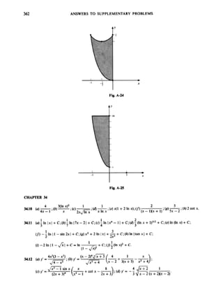
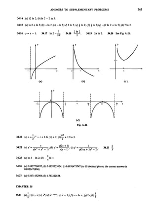
””’;
X
(e)
Y (-1 +-)1 =
2x +3
2 x + l x + 2 2 J r n ) ‘](https://image.slidesharecdn.com/problemscalculus-221128025033-038ef06f/85/problems-calculus-pdf-377-320.jpg)
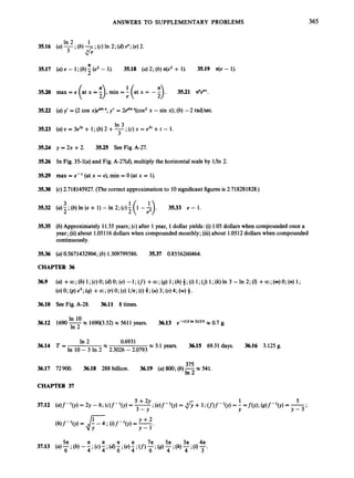
![ANSWERS TO SUPPLEMENTARY PROBLEMS 367
3 12 2
5 5
3
7
.
1
5 (a)- ;(b)-;(c) 15(2 - 3$); (d) (fi- 1); (e)0
.
3
7
.
1
6 Domain = (- 00, 00)' range = (0'13.
R 5a/2 for x 5 -1.
2 ' for x 2 1 '
37.17 (a) sin-' x +cos-' x = - (b) tan-' x +cot-' x =- * (c) sec-' x +csc- 'x = {
(d)tan-' x +tan-' - = - or cot-' x = tan-' -
1). 2 '
x 2 X
X 1 sin x . -3
( 2 f i ) J G ; (c) - 1 +cos2 x ' (1 +9x2)cot-' 3x;
37.18 (U) -
+tan-' x;
1+x2
1
1 p Jc7 ifx>O
i f x c o
(e) ,.(cos-1 x - ;
) (tan-' xX1 +x2);
(h)[ 2 J ; n
2x2
i f a > o
i f a < O
'
1
(i) -
-
1+ x 2 '
u + v
3
7
.
1
9 tan-' u +tan-' v = tan-' -
1-uv'
1 1 3x X 1 4x
2 2 6 2 5 4 5
3
7
.
2
0 (a)- tan-' +C;(b)- tan-' -+ C;(c)sin-' - +C;(d)- sin-' -+C;(e)sec-' (x - 3) +C;
1 X 1 3x
2 2 4 4
(qx)
+C; (h) - sec-' - +C; (i) -sec-' -+C;
1 sin-' (T)
d x +c;(g) -tan-' -
Jr;i
1 x + 4
(n)2(3 sin-' 9
- ,/-) +C; (o)zln(x2+8x +20) - 2 tan-' -+C;
2
1 X2 1 ex 1
8 J stan-' - + C; (4)
- sin-' -+C; (r)- tan-' -+C; (s)-tan-'
X2
2 2 fi
Jj 2 2
(p) 2 +2x --
3
(t)-
1tan-' -
x + l + C .
3 3
mi/min = 5000~
mi/h FZ 15708 mi/h.
1 25On
3
7
.
2
1 y = - x. 3
7
.
2
2 -1 rad/sec. 3
7
.
2
3 -
3 3
R R R2
4' 6' 3 '
3
7
.
2
4 - 3
7
.
2
5 - 3
7
.
2
6 - 3
7
.
2
8 2
,
/
i ft.
3
7
.
2
9 (a)[-;,;];(b)[O,~];(c)[-l,l];(d) -1 5 x 5 l;(e) -1 5 x 5 1.
y(1 +y2)(2x-tan-' Y
3
7
.
3
0 (U)
1+y2+xy](https://image.slidesharecdn.com/problemscalculus-221128025033-038ef06f/85/problems-calculus-pdf-380-320.jpg)
![368 ANSWERS TO SUPPLEMENTARY PROBLEMS
A
3731 See Fig. A-29. 3733 -
16'
t'
Fig. A-29
3734 (b) 3.141592651. (Thecorrect approximationto 10 significantfiguresis 3.141592654.)
CHAPTER 38
e"(sin x -cos x)
2
+C; (c) ex(x3- 3x2+6x - 6) +C;
3
8
.
6 (a) -eex(x2 +2x +2) +C; (b)
(d)x sin-' x +,
/
- +C; (e) x sin x +cos x +C; (I)
2x sin x +(cos x)(2 - x') +C;
(g)- [cos (In x) +sin (In x)] +C; (h) -[5x sin (5x - 1) +cos (Sx - l)]
+C;
X 1
2 25
eu 1
(b sin bx +U cos bx) +C; ( j )- (x - sin x cos x) +C;
(0 2
e3*
9
sin3x sin x
+c = -(2 +cos2 x) +C; (01 x +sin 2x + +c;(rn)-(3x - 1) + C;
3 4 (I
(k) sin x --
3
1
8
(n) x tan x - In Isec x I+C;(0)-(2x2+2x sin 2x - cos 2x) +C;
(p) xOn x ) ~
- 2x(h x - 1) +C;
1 1 1 e3x
2 X 27
(q)4(sin 2x -2x cos 2x) +C;(r) --cos x2 +C;(s) -- (1 +In x) +C;(t)-(9x2 - 6x +2) +C;
1
6
(U)- [2x3 tan- 'x -x2 +In (1 +x2)] +C; (U)x In (x2+ 1) - 2(x - tan-' x) +C;
x3
9
- 2) + C;(x) -(3 In x - 1) +C.
A
3
8
.
7 (a) 1;(b) (i) n(e -2); (ii)-(1 +e2).
2
A2 2
A
2 n
1
3
8
.
8 (U) j;(b) 2 ~ ;
(c)A . 3
8
.
1
0 (U)- ;(b) 2z2. 3
8
.
1
1 (U) 0;(b) --.
cosn-' x sin x ~ n - 1Jcosn-2
38.12 (a) Icos" x dx = x dx.
n n
sinn-' x cos x + n - 1
(b) I s i d x dx = - x dx.
n n
sec"-2 x tan x n - 2
I n - 1 n - 1
3
8
.
1
3 (a) sec"xdx= +-I s e C 2x dx;
sec2x tan x 2
3 3
+- tan x +C = (tan x)
1
2
(b) (i)-(sec x tan x +In Isec x +tan x I)+C; (ii)](https://image.slidesharecdn.com/problemscalculus-221128025033-038ef06f/85/problems-calculus-pdf-381-320.jpg)
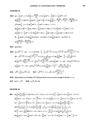
![370 ANSWERS TO SUPPLEMENTARY PROBLEMS
x2 1 1 1 1
2 9 2 2 x + 1
(0)- +- Dn 1x1-41 In (x2 +9)] +C;(p)In 1x1--In (x2 + 1)+
-
,
+ C;
1 1 x 1 x - 4
(4)
25In Ix - 1I --I
n (x2 +
50
x + l
+c;(s) ln 1-1x + 2 +c ;
1
2
(r)InIx(--In(x2+x+1)-
1 11
3
(t)? In Ixl +-In Ix +3I - 3 In Ix +21 +C;(U) x - In (1 +e? + C.
+c.
1 1
40.8 (a)81(3 In 2 +x d ) ; (6)5( n f i-3 In 2). 40.9
X
1 -tan -
2
40.10 (a)In(l -sinx)+C;(b)ln(sinx- l ( + C ; ( c ) s i n x < l .](https://image.slidesharecdn.com/problemscalculus-221128025033-038ef06f/85/problems-calculus-pdf-383-320.jpg)

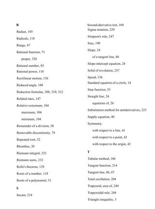
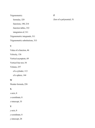

This document introduces coordinate systems on a line. It defines how to assign coordinates to points on a line by choosing an origin point and direction, and measuring distances from the origin. Points to the right of the origin have positive coordinates equal to their distance from the origin, while points to the left have negative coordinates equal to the negative of their distance. The absolute value of a real number is defined as its magnitude, regardless of sign.


![[Sundstrom_Ted.]_Mathematical_Reasoning_Writing - Copy.pdf](https://cdn.slidesharecdn.com/ss_thumbnails/sundstromted-221124155318-3b41c59e-thumbnail.jpg?width=640&height=640&fit=bounds)


