This document provides publication information for Thomas' Calculus: Early Transcendentals, Thirteenth Edition. It lists the authors and editors who contributed to revising and updating the textbook. It also provides copyright information and includes a brief table of contents that outlines the chapters and topics covered in the book.

1. Based on the original work by
George B. Thomas, Jr.
Massachusetts Institute of Technology
as revised by
Maurice D. Weir
Naval Postgraduate School
Joel Hass
University of California, Davis
with the assistance of
Christopher Heil
Georgia Institute of Technology
Thomas’
Calculus
Early Transcendentals
Thirteenth Edition
Boston Columbus Indianapolis New York San Francisco Upper Saddle River
Amsterdam Cape Town Dubai London Madrid Milan Munich Paris Montréal Toronto
Delhi Mexico City São Paulo Sydney Hong Kong Seoul Singapore Taipei Tokyo

2. Editor-in-Chief: Deirdre Lynch
Senior Acquisitions Editor: William Hoffman
Senior Content Editor: Rachel S. Reeve
Senior Managing Editor: Karen Wernholm
Associate Managing Editor: Tamela Ambush
Senior Production Project Manager: Sheila Spinney; Sherry Berg
Associate Design Director, USHE EMSS, TED and HSC: Andrea Nix
Art Director and Cover Design: Beth Paquin
Digital Assets Manager: Marianne Groth
Associate Producer Multimedia: Nicholas Sweeny
Software Development: John Flanagan and Kristina Evans
Executive Marketing Manager: Jeff Weidenaar
Marketing Assistant: Caitlin Crain
Senior Author Support/Technology Specialist: Joe Vetere
Manufacturing Manager: Carol Melville
Text Design, Production Coordination, Composition: Cenveo®
Publisher Services
Illustrations: Karen Hartpence, IlustraTech; Cenveo®
Publisher Services
Cover image: Art on File/Corbis
For permission to use copyrighted material, grateful acknowledgment is made to the copyright holders on
page C-1, which is hereby made part of this copyright page.
Many of the designations used by manufacturers and sellers to distinguish their products are claimed as trademarks.
Where those designations appear in this book, and Pearson Education was aware of a trademark claim, the designa-
tions have been printed in initial caps or all caps.
Library of Congress Cataloging-in-Publication Data
Weir, Maurice D.
Thomas’ calculus : early transcendentals : based on the original work by George B. Thomas, Jr., Massachusetts
Institute of Technology.—Thirteenth edition / as revised by Maurice D. Weir, Naval Postgraduate School, Joel
Hass, University of California, Davis.
pages cm
ISBN 978-0-321-88407-7 (hardcover)
I. Hass, Joel. II. Thomas, George B. (George Brinton), Jr., 1914–2006. Calculus. Based on (Work): III.
Title. IV. Title: Calculus.
QA303.2.W45 2014
515–dc23 2013023096
Copyright © 2014, 2010, 2008 Pearson Education, Inc. All rights reserved. No part of this publication may be
reproduced, stored in a retrieval system, or transmitted, in any form or by any means, electronic, mechanical,
photocopying, recording, or otherwise, without the prior written permission of the publisher. Printed in the United
States of America. For information on obtaining permission for use of material in this work, please submit a written
request to Pearson Education, Inc., Rights and Contracts Department, 501 Boylston Street, Suite 900, Boston, MA 02116,
fax your request to 617-848-7047, or e-mail at http://www.pearsoned.com/legal/permissions.htm.
1 2 3 4 5 6 7 8 9 10—CRK—17 16 15 14 13
www.pearsonhighered.com
ISBN-10: 0-321-88407-8
ISBN-13: 978-0-321-88407-7

3. iii
Preface ix
1 Functions 1
1.1 Functions and Their Graphs 1
1.2 Combining Functions; Shifting and Scaling Graphs 14
1.3 Trigonometric Functions 21
1.4 Graphing with Software 29
1.5 Exponential Functions 36
1.6 Inverse Functions and Logarithms 41
Questions to Guide Your Review 54
Practice Exercises 54
Additional and Advanced Exercises 57
2 Limits and Continuity 59
2.1 Rates of Change and Tangents to Curves 59
2.2 Limit of a Function and Limit Laws 66
2.3 The Precise Definition of a Limit 77
2.4 One-Sided Limits 86
2.5 Continuity 93
2.6 Limits Involving Infinity; Asymptotes of Graphs 104
Questions to Guide Your Review 118
Practice Exercises 118
Additional and Advanced Exercises 120
3 Derivatives 123
3.1 Tangents and the Derivative at a Point 123
3.2 The Derivative as a Function 128
3.3 Differentiation Rules 136
3.4 The Derivative as a Rate of Change 146
3.5 Derivatives of Trigonometric Functions 156
3.6 The Chain Rule 163
3.7 Implicit Differentiation 171
3.8 Derivatives of Inverse Functions and Logarithms 177
3.9 Inverse Trigonometric Functions 187
3.10 Related Rates 193
3.11 Linearization and Differentials 202
Questions to Guide Your Review 214
Practice Exercises 215
Additional and Advanced Exercises 219
Contents

4. iv Contents
4 Applications of Derivatives 223
4.1 Extreme Values of Functions 223
4.2 The Mean Value Theorem 231
4.3 Monotonic Functions and the First Derivative Test 239
4.4 Concavity and Curve Sketching 244
4.5 Indeterminate Forms and L’Hôpital’s Rule 255
4.6 Applied Optimization 264
4.7 Newton’s Method 276
4.8 Antiderivatives 281
Questions to Guide Your Review 291
Practice Exercises 291
Additional and Advanced Exercises 295
5 Integrals 299
5.1 Area and Estimating with Finite Sums 299
5.2 Sigma Notation and Limits of Finite Sums 309
5.3 The Definite Integral 316
5.4 The Fundamental Theorem of Calculus 328
5.5 Indefinite Integrals and the Substitution Method 339
5.6 Definite Integral Substitutions and the Area Between Curves 347
Questions to Guide Your Review 357
Practice Exercises 357
Additional and Advanced Exercises 361
6 Applications of Definite Integrals 365
6.1 Volumes Using Cross-Sections 365
6.2 Volumes Using Cylindrical Shells 376
6.3 Arc Length 384
6.4 Areas of Surfaces of Revolution 390
6.5 Work and Fluid Forces 395
6.6 Moments and Centers of Mass 404
Questions to Guide Your Review 415
Practice Exercises 416
Additional and Advanced Exercises 417
7 Integrals and Transcendental Functions 420
7.1 The Logarithm Defined as an Integral 420
7.2 Exponential Change and Separable Differential Equations 430
7.3 Hyperbolic Functions 439
7.4 Relative Rates of Growth 448
Questions to Guide Your Review 453
Practice Exercises 453
Additional and Advanced Exercises 455

5. Contents v
8 Techniques of Integration 456
8.1 Using Basic Integration Formulas 456
8.2 Integration by Parts 461
8.3 Trigonometric Integrals 469
8.4 Trigonometric Substitutions 475
8.5 Integration of Rational Functions by Partial Fractions 480
8.6 Integral Tables and Computer Algebra Systems 489
8.7 Numerical Integration 494
8.8 Improper Integrals 504
8.9 Probability 515
Questions to Guide Your Review 528
Practice Exercises 529
Additional and Advanced Exercises 531
9 First-Order Differential Equations 536
9.1 Solutions, Slope Fields, and Euler’s Method 536
9.2 First-Order Linear Equations 544
9.3 Applications 550
9.4 Graphical Solutions of Autonomous Equations 556
9.5 Systems of Equations and Phase Planes 563
Questions to Guide Your Review 569
Practice Exercises 569
Additional and Advanced Exercises 570
10 Infinite Sequences and Series 572
10.1 Sequences 572
10.2 Infinite Series 584
10.3 The Integral Test 593
10.4 Comparison Tests 600
10.5 Absolute Convergence; The Ratio and Root Tests 604
10.6 Alternating Series and Conditional Convergence 610
10.7 Power Series 616
10.8 Taylor and Maclaurin Series 626
10.9 Convergence of Taylor Series 631
10.10 The Binomial Series and Applications of Taylor Series 638
Questions to Guide Your Review 647
Practice Exercises 648
Additional and Advanced Exercises 650
11 Parametric Equations and Polar Coordinates 653
11.1 Parametrizations of Plane Curves 653
11.2 Calculus with Parametric Curves 661
11.3 Polar Coordinates 671

6. vi Contents
11.4 Graphing Polar Coordinate Equations 675
11.5 Areas and Lengths in Polar Coordinates 679
11.6 Conic Sections 683
11.7 Conics in Polar Coordinates 692
Questions to Guide Your Review 699
Practice Exercises 699
Additional and Advanced Exercises 701
12 Vectors and the Geometry of Space 704
12.1 Three-Dimensional Coordinate Systems 704
12.2 Vectors 709
12.3 The Dot Product 718
12.4 The Cross Product 726
12.5 Lines and Planes in Space 732
12.6 Cylinders and Quadric Surfaces 740
Questions to Guide Your Review 745
Practice Exercises 746
Additional and Advanced Exercises 748
13 Vector-Valued Functions and Motion in Space 751
13.1 Curves in Space and Their Tangents 751
13.2 Integrals of Vector Functions; Projectile Motion 759
13.3 Arc Length in Space 768
13.4 Curvature and Normal Vectors of a Curve 772
13.5 Tangential and Normal Components of Acceleration 778
13.6 Velocity and Acceleration in Polar Coordinates 784
Questions to Guide Your Review 788
Practice Exercises 788
Additional and Advanced Exercises 790
14 Partial Derivatives 793
14.1 Functions of Several Variables 793
14.2 Limits and Continuity in Higher Dimensions 801
14.3 Partial Derivatives 810
14.4 The Chain Rule 821
14.5 Directional Derivatives and Gradient Vectors 830
14.6 Tangent Planes and Differentials 839
14.7 Extreme Values and Saddle Points 848
14.8 Lagrange Multipliers 857
14.9 Taylor’s Formula for Two Variables 866
14.10 Partial Derivatives with Constrained Variables 870
Questions to Guide Your Review 875
Practice Exercises 876
Additional and Advanced Exercises 879

7. Contents vii
15 Multiple Integrals 882
15.1 Double and Iterated Integrals over Rectangles 882
15.2 Double Integrals over General Regions 887
15.3 Area by Double Integration 896
15.4 Double Integrals in Polar Form 900
15.5 Triple Integrals in Rectangular Coordinates 906
15.6 Moments and Centers of Mass 915
15.7 Triple Integrals in Cylindrical and Spherical Coordinates 922
15.8 Substitutions in Multiple Integrals 934
Questions to Guide Your Review 944
Practice Exercises 944
Additional and Advanced Exercises 947
16 Integrals and Vector Fields 950
16.1 Line Integrals 950
16.2 Vector Fields and Line Integrals: Work, Circulation, and Flux 957
16.3 Path Independence, Conservative Fields, and Potential Functions 969
16.4 Green’s Theorem in the Plane 980
16.5 Surfaces and Area 992
16.6 Surface Integrals 1003
16.7 Stokes’ Theorem 1014
16.8 The Divergence Theorem and a Unified Theory 1027
Questions to Guide Your Review 1039
Practice Exercises 1040
Additional and Advanced Exercises 1042
17 Second-Order Differential Equations online
17.1 Second-Order Linear Equations
17.2 Nonhomogeneous Linear Equations
17.3 Applications
17.4 Euler Equations
17.5 Power Series Solutions
Appendices AP-1
A.1 Real Numbers and the Real Line AP-1
A.2 Mathematical Induction AP-6
A.3 Lines, Circles, and Parabolas AP-10
A.4 Proofs of Limit Theorems AP-19
A.5 Commonly Occurring Limits AP-22
A.6 Theory of the Real Numbers AP-23
A.7 Complex Numbers AP-26
A.8 The Distributive Law for Vector Cross Products AP-35
A.9 The Mixed Derivative Theorem and the Increment Theorem AP-36
Answers to Odd-Numbered Exercises A-1
Index I-1
Credits C-1
A Brief Table of Integrals T-1

8. This page intentionally left blank

9. ix
Thomas’ Calculus: Early Transcendentals, Thirteenth Edition, provides a modern intro-
duction to calculus that focuses on conceptual understanding in developing the essential
elements of a traditional course. This material supports a three-semester or four-quarter
calculus sequence typically taken by students in mathematics, engineering, and the natural
sciences. Precise explanations, thoughtfully chosen examples, superior figures, and time-
tested exercise sets are the foundation of this text. We continue to improve this text in
keeping with shifts in both the preparation and the ambitions of today’s students, and the
applications of calculus to a changing world.
Many of today’s students have been exposed to the terminology and computational
methods of calculus in high school. Despite this familiarity, their acquired algebra and
trigonometry skills sometimes limit their ability to master calculus at the college level. In
this text, we seek to balance students’ prior experience in calculus with the algebraic skill
development they may still need, without slowing their progress through calculus itself. We
have taken care to provide enough review material (in the text and appendices), detailed
solutions, and variety of examples and exercises, to support a complete understanding of
calculus for students at varying levels. We present the material in a way to encourage stu-
dent thinking, going beyond memorizing formulas and routine procedures, and we show
students how to generalize key concepts once they are introduced. References are made
throughout which tie a new concept to a related one that was studied earlier, or to a gen-
eralization they will see later on. After studying calculus from Thomas, students will have
developed problem solving and reasoning abilities that will serve them well in many im-
portant aspects of their lives. Mastering this beautiful and creative subject, with its many
practical applications across so many fields of endeavor, is its own reward. But the real gift
of studying calculus is acquiring the ability to think logically and factually, and learning
how to generalize conceptually. We intend this book to encourage and support those goals.
New to this Edition
In this new edition we further blend conceptual thinking with the overall logic and struc-
ture of single and multivariable calculus. We continue to improve clarity and precision,
taking into account helpful suggestions from readers and users of our previous texts. While
keeping a careful eye on length, we have created additional examples throughout the text.
Numerous new exercises have been added at all levels of difficulty, but the focus in this
revision has been on the mid-level exercises. A number of figures have been reworked and
new ones added to improve visualization. We have written a new section on probability,
which provides an important application of integration to the life sciences.
We have maintained the basic structure of the Table of Contents, and retained im-
provements from the twelfth edition. In keeping with this process, we have added more
improvements throughout, which we detail here:
Preface

10. x Preface
• Functions In discussing the use of software for graphing purposes, we added a brief
subsection on least squares curve fitting, which allows students to take advantage of
this widely used and available application. Prerequisite material continues to be re-
viewed in Appendices 1–3.
• Continuity We clarified the continuity definitions by confining the term “endpoints” to
intervals instead of more general domains, and we moved the subsection on continuous
extension of a function to the end of the continuity section.
• Derivatives We included a brief geometric insight justifying l’Hôpital’s Rule. We also
enhanced and clarified the meaning of differentiability for functions of several vari-
ables, and added a result on the Chain Rule for functions defined along a path.
• Integrals We wrote a new section reviewing basic integration formulas and the Sub-
stitution Rule, using them in combination with algebraic and trigonometric identities,
before presenting other techniques of integration.
• Probability We created a new section applying improper integrals to some commonly
used probability distributions, including the exponential and normal distributions.
Many examples and exercises apply to the life sciences.
• Series We now present the idea of absolute convergence before giving the Ratio and
Root Tests, and then state these tests in their stronger form. Conditional convergence is
introduced later on with the Alternating Series Test.
• Multivariable and Vector Calculus We give more geometric insight into the idea of
multiple integrals, and we enhance the meaning of the Jacobian in using substitutions
to evaluate them. The idea of surface integrals of vector fields now parallels the notion
for line integrals of vector fields. We have improved our discussion of the divergence
and curl of a vector field.
• Exercises and Examples Strong exercise sets are traditional with Thomas’ Calculus,
and we continue to strengthen them with each new edition. Here, we have updated,
changed, and added many new exercises and examples, with particular attention to in-
cluding more applications to the life science areas and to contemporary problems. For
instance, we updated an exercise on the growth of the U.S. GNP and added new exer-
cises addressing drug concentrations and dosages, estimating the spill rate of a ruptured
oil pipeline, and predicting rising costs for college tuition.
Continuing Features
RIGOR The level of rigor is consistent with that of earlier editions. We continue to distin-
guish between formal and informal discussions and to point out their differences. We think
starting with a more intuitive, less formal, approach helps students understand a new or dif-
ficult concept so they can then appreciate its full mathematical precision and outcomes. We
pay attention to defining ideas carefully and to proving theorems appropriate for calculus
students, while mentioning deeper or subtler issues they would study in a more advanced
course. Our organization and distinctions between informal and formal discussions give the
instructor a degree of flexibility in the amount and depth of coverage of the various top-
ics. For example, while we do not prove the Intermediate Value Theorem or the Extreme
Value Theorem for continuous functions on a # x # b, we do state these theorems precisely,
illustrate their meanings in numerous examples, and use them to prove other important re-
sults. Furthermore, for those instructors who desire greater depth of coverage, in Appendix
6 we discuss the reliance of the validity of these theorems on the completeness of the real
numbers.

11. Preface xi
WRITING EXERCISES Writing exercises placed throughout the text ask students to ex-
plore and explain a variety of calculus concepts and applications. In addition, the end of
each chapter contains a list of questions for students to review and summarize what they
have learned. Many of these exercises make good writing assignments.
END-OF-CHAPTER REVIEWS AND PROJECTS In addition to problems appearing after
each section, each chapter culminates with review questions, practice exercises covering
the entire chapter, and a series of Additional and Advanced Exercises serving to include
more challenging or synthesizing problems. Most chapters also include descriptions of
several Technology Application Projects that can be worked by individual students or
groups of students over a longer period of time. These projects require the use of a com-
puter running Mathematica or Maple and additional material that is available over the
Internet at www.pearsonhighered.com/thomas and in MyMathLab.
WRITING AND APPLICATIONS As always, this text continues to be easy to read, conversa-
tional, and mathematically rich. Each new topic is motivated by clear, easy-to-understand
examples and is then reinforced by its application to real-world problems of immediate
interest to students. A hallmark of this book has been the application of calculus to science
and engineering. These applied problems have been updated, improved, and extended con-
tinually over the last several editions.
TECHNOLOGY In a course using the text, technology can be incorporated according to
the taste of the instructor. Each section contains exercises requiring the use of technology;
these are marked with a T if suitable for calculator or computer use, or they are labeled
Computer Explorations if a computer algebra system (CAS, such as Maple or Math-
ematica) is required.
Additional Resources
INSTRUCTOR’S SOLUTIONS MANUAL
Single Variable Calculus (Chapters 1–11), ISBN 0-321-88408-6 | 978-0-321-88408-4
Multivariable Calculus (Chapters 10–16), ISBN 0-321-87901-5 | 978-0-321-87901-1
The Instructor’s Solutions Manual contains complete worked-out solutions to all of the
exercises in Thomas’Calculus: Early Transcendentals.
STUDENT’S SOLUTIONS MANUAL
Single Variable Calculus (Chapters 1–11), ISBN 0-321-88410-8 | 978-0-321-88410-7
Multivariable Calculus (Chapters 10–16), ISBN 0-321-87897-3 | 978-0-321-87897-7
The Student’s Solutions Manual is designed for the student and contains carefully
worked-out solutions to all the odd-numbered exercises in Thomas’ Calculus: Early
Transcendentals.
JUST-IN-TIME ALGEBRA AND TRIGONOMETRY FOR
EARLY TRANSCENDENTALS CALCULUS, Fourth Edition
ISBN 0-321-67103-1 | 978-0-321-67103-5
Sharp algebra and trigonometry skills are critical to mastering calculus, and Just-in-Time
Algebra and Trigonometry for Early Transcendentals Calculus by Guntram Mueller and
Ronald I. Brent is designed to bolster these skills while students study calculus. As stu-
dents make their way through calculus, this text is with them every step of the way, show-
ing them the necessary algebra or trigonometry topics and pointing out potential problem
spots. The easy-to-use table of contents has algebra and trigonometry topics arranged in
the order in which students will need them as they study calculus.

12. xii Preface
Technology Resource Manuals
Maple Manual by Marie Vanisko, Carroll College
Mathematica Manual by Marie Vanisko, Carroll College
TI-Graphing Calculator Manual by Elaine McDonald-Newman, Sonoma State University
These manuals cover Maple 17, Mathematica 8, and the TI-83 Plus/TI-84 Plus and TI-89,
respectively. Each manual provides detailed guidance for integrating a specific software
package or graphing calculator throughout the course, including syntax and commands.
These manuals are available to qualified instructors through the Thomas’ Calculus: Early
Transcendentals Web site, www.pearsonhighered.com/thomas, and MyMathLab.
WEB SITE www.pearsonhighered.com/thomas
The Thomas’ Calculus: Early Transcendentals Web site contains the chapter on Second-
Order Differential Equations, including odd-numbered answers, and provides the ex-
panded historical biographies and essays referenced in the text. The Technology Resource
Manuals and the Technology Application Projects, which can be used as projects by in-
dividual students or groups of students, are also available.
MyMathLab®
Online Course (access code required)
MyMathLab from Pearson is the world’s leading online resource in mathematics, integrat-
ing interactive homework, assessment, and media in a flexible, easy-to-use format.
MyMathLab delivers proven results in helping individual students succeed.
• MyMathLab has a consistently positive impact on the quality of learning in higher
education math instruction. MyMathLab can be successfully implemented in any
environment—lab-based, hybrid, fully online, traditional—and demonstrates the quan-
tifiable difference that integrated usage makes in regard to student retention, subse-
quent success, and overall achievement.
• MyMathLab’s comprehensive online gradebook automatically tracks your students’ re-
sults on tests, quizzes, homework, and in the study plan. You can use the gradebook to
quickly intervene if your students have trouble, or to provide positive feedback on a job
well done. The data within MyMathLab are easily exported to a variety of spreadsheet
programs, such as Microsoft Excel. You can determine which points of data you want
to export, and then analyze the results to determine success.
MyMathLab provides engaging experiences that personalize, stimulate, and measure
learning for each student.
• “Getting Ready” chapter includes hundreds of exercises that address prerequisite
skills in algebra and trigonometry. Each student can receive remediation for just those
skills he or she needs help with.
• Exercises: The homework and practice exercises in MyMathLab are correlated to the
exercises in the textbook, and they regenerate algorithmically to give students unlim-
ited opportunity for practice and mastery. The software offers immediate, helpful feed-
back when students enter incorrect answers.
• Multimedia Learning Aids: Exercises include guided solutions, sample problems,
animations, Java™ applets, videos, and eText access for extra help at point-of-use.
• Expert Tutoring: Although many students describe the whole of MyMathLab as “like
having your own personal tutor,” students using MyMathLab do have access to live
tutoring from Pearson, from qualified math and statistics instructors.

13. Preface xiii
And, MyMathLab comes from an experienced partner with educational expertise and an
eye on the future.
• Knowing that you are using a Pearson product means knowing that you are using qual-
ity content. It means that our eTexts are accurate and our assessment tools work. It also
means we are committed to making MyMathLab as accessible as possible.
• Whether you are just getting started with MyMathLab, or have a question along the
way, we’re here to help you learn about our technologies and how to incorporate them
into your course.
To learn more about how MyMathLab combines proven learning applications with power-
ful assessment, visit www.mymathlab.com or contact your Pearson representative.
Video Lectures with Optional Captioning
The Video Lectures with Optional Captioning feature an engaging team of mathemat-
ics instructors who present comprehensive coverage of topics in the text. The lecturers’
presentations include examples and exercises from the text and support an approach that
emphasizes visualization and problem solving. Available only through MyMathLab and
MathXL.
MathXL®
Online Course (access code required)
MathXL®
is the homework and assessment engine that runs MyMathLab. (MyMathLab is
MathXL plus a learning management system.)
With MathXL, instructors can:
• Create, edit, and assign online homework and tests using algorithmically generated ex-
ercises correlated at the objective level to the textbook.
• Create and assign their own online exercises and import TestGen tests for added flexibility.
• Maintain records of all student work tracked in MathXL’s online gradebook.
With MathXL, students can:
• Take chapter tests in MathXL and receive personalized study plans and/or personalized
homework assignments based on their test results.
• Use the study plan and/or the homework to link directly to tutorial exercises for the
objectives they need to study.
• Access supplemental animations and video clips directly from selected exercises.
MathXL is available to qualified adopters. For more information, visit our website at
www.mathxl.com, or contact your Pearson representative.
TestGen®
TestGen®
(www.pearsoned.com/testgen) enables instructors to build, edit, print, and ad-
minister tests using a computerized bank of questions developed to cover all the objec-
tives of the text. TestGen is algorithmically based, allowing instructors to create multiple
but equivalent versions of the same question or test with the click of a button. Instructors
can also modify test bank questions or add new questions. The software and test bank are
available for download from Pearson Education’s online catalog.
PowerPoint®
Lecture Slides
These classroom presentation slides are geared specifically to the sequence and philosophy
of the Thomas’Calculus series. Key graphics from the book are included to help bring the
concepts alive in the classroom.These files are available to qualified instructors through
the Pearson Instructor Resource Center, www.pearsonhighered/irc, and MyMathLab.

14. xiv Preface
Acknowledgments
We would like to express our thanks to the people who made many valuable contributions
to this edition as it developed through its various stages:
Accuracy Checkers
Lisa Collette
Patricia Nelson
Tom Wegleitner
Reviewers for Recent Editions
Meighan Dillon, Southern Polytechnic State University
Anne Dougherty, University of Colorado
Said Fariabi, San Antonio College
Klaus Fischer, George Mason University
Tim Flood, Pittsburg State University
Rick Ford, California State University—Chico
Robert Gardner, East Tennessee State University
Christopher Heil, Georgia Institute of Technology
Joshua Brandon Holden, Rose-Hulman Institute of Technology
Alexander Hulpke, Colorado State University
Jacqueline Jensen, Sam Houston State University
Jennifer M. Johnson, Princeton University
Hideaki Kaneko, Old Dominion University
Przemo Kranz, University of Mississippi
Xin Li, University of Central Florida
Maura Mast, University of Massachusetts—Boston
Val Mohanakumar, Hillsborough Community College—Dale Mabry Campus
Aaron Montgomery, Central Washington University
Christopher M. Pavone, California State University at Chico
Cynthia Piez, University of Idaho
Brooke Quinlan, Hillsborough Community College—Dale Mabry Campus
Rebecca A. Segal, Virginia Commonwealth University
Andrew V. Sills, Georgia Southern University
Alex Smith, University of Wisconsin—Eau Claire
Mark A. Smith, Miami University
Donald Solomon, University of Wisconsin—Milwaukee
John Sullivan, Black Hawk College
Maria Terrell, Cornell University
Blake Thornton, Washington University in St. Louis
David Walnut, George Mason University
Adrian Wilson, University of Montevallo
Bobby Winters, Pittsburg State University
Dennis Wortman, University of Massachusetts—Boston

15. 1
OVERVIEW Functions are fundamental to the study of calculus. In this chapter we review
what functions are and how they are pictured as graphs, how they are combined and trans-
formed, and ways they can be classified. We review the trigonometric functions, and we
discuss misrepresentations that can occur when using calculators and computers to obtain
a function’s graph. We also discuss inverse, exponential, and logarithmic functions. The
real number system, Cartesian coordinates, straight lines, circles, parabolas, and ellipses
are reviewed in the Appendices.
Functions
1
1.1 Functions and Their Graphs
Functions are a tool for describing the real world in mathematical terms. A function can be
represented by an equation, a graph, a numerical table, or a verbal description; we will use
all four representations throughout this book. This section reviews these function ideas.
Functions; Domain and Range
The temperature at which water boils depends on the elevation above sea level (the boiling
point drops as you ascend). The interest paid on a cash investment depends on the length of
time the investment is held. The area of a circle depends on the radius of the circle. The dis-
tance an object travels at constant speed along a straight-line path depends on the elapsed time.
In each case, the value of one variable quantity, say y, depends on the value of another
variable quantity, which we might call x. We say that “y is a function of x” and write this
symbolically as
y = ƒ(x) (“y equals ƒ of x”).
In this notation, the symbol ƒ represents the function, the letter x is the independent variable
representing the input value of ƒ, and y is the dependent variable or output value of ƒ at x.
DEFINITION A function ƒ from a set D to a set Y is a rule that assigns a unique
(single) element ƒ(x)∊Y to each element x∊D.
The set D of all possible input values is called the domain of the function. The set of
all output values of ƒ(x) as x varies throughout D is called the range of the function. The
range may not include every element in the set Y. The domain and range of a function can
be any sets of objects, but often in calculus they are sets of real numbers interpreted as
points of a coordinate line. (In Chapters 13–16, we will encounter functions for which the
elements of the sets are points in the coordinate plane or in space.)

16. 2 Chapter 1: Functions
Often a function is given by a formula that describes how to calculate the output value
from the input variable. For instance, the equation A = pr2
is a rule that calculates the
area A of a circle from its radius r (so r, interpreted as a length, can only be positive in this
formula). When we define a function y = ƒ(x) with a formula and the domain is not stated
explicitly or restricted by context, the domain is assumed to be the largest set of real
x-values for which the formula gives real y-values, which is called the natural domain. If
we want to restrict the domain in some way, we must say so. The domain of y = x2
is the
entire set of real numbers. To restrict the domain of the function to, say, positive values of
x, we would write “y = x2
, x 7 0.”
Changing the domain to which we apply a formula usually changes the range as well.
The range of y = x2
is [0, q). The range of y = x2
, x Ú 2, is the set of all numbers
obtained by squaring numbers greater than or equal to 2. In set notation (see Appendix 1),
the range is 5x2
x Ú 26 or 5y y Ú 46 or 34, q).
When the range of a function is a set of real numbers, the function is said to be real-
valued. The domains and ranges of most real-valued functions of a real variable we con-
sider are intervals or combinations of intervals. The intervals may be open, closed, or half
open, and may be finite or infinite. Sometimes the range of a function is not easy to find.
A function ƒ is like a machine that produces an output value ƒ(x) in its range whenever we
feed it an input value x from its domain (Figure 1.1). The function keys on a calculator give an
example of a function as a machine. For instance, the 2x key on a calculator gives an output
value (the square root) whenever you enter a nonnegative number x and press the 2x key.
A function can also be pictured as an arrow diagram (Figure 1.2). Each arrow associates
an element of the domain D with a unique or single element in the set Y. In Figure 1.2, the
arrows indicate that ƒ(a) is associated with a, ƒ(x) is associated with x, and so on. Notice that
a function can have the same value at two different input elements in the domain (as occurs
with ƒ(a) in Figure 1.2), but each input element x is assigned a single output value ƒ(x).
EXAMPLE 1 Let’s verify the natural domains and associated ranges of some simple
functions. The domains in each case are the values of x for which the formula makes sense.
Input
(domain)
Output
(range)
x f(x)
f
FIGURE 1.1 A diagram showing a
function as a kind of machine.
x
a f(a) f(x)
D = domain set Y = set containing
the range
FIGURE 1.2 A function from a set D
to a set Y assigns a unique element of Y
to each element in D.
Function Domain (x) Range (y)
y = x2
(-q, q) 30, q)
y = 1x (-q, 0) ∪ (0, q) (-q, 0) ∪ (0, q)
y = 2x 30, q) 30, q)
y = 24 - x (-q, 44 30, q)
y = 21 - x2
3-1, 14 30, 14
Solution The formula y = x2
gives a real y-value for any real number x, so the domain
is (-q, q). The range of y = x2
is 30, q) because the square of any real number is non-
negative and every nonnegative number y is the square of its own square root, y = 12y22
for y Ú 0.
The formula y = 1x gives a real y-value for every x except x = 0. For consistency
in the rules of arithmetic, we cannot divide any number by zero. The range of y = 1x, the
set of reciprocals of all nonzero real numbers, is the set of all nonzero real numbers, since
y = 1(1y). That is, for y ≠ 0 the number x = 1y is the input assigned to the output
value y.
The formula y = 2x gives a real y-value only if x Ú 0. The range of y = 2x is
30, q) because every nonnegative number is some number’s square root (namely, it is the
square root of its own square).
In y = 24 - x, the quantity 4 - x cannot be negative. That is, 4 - x Ú 0, or
x … 4. The formula gives real y-values for all x … 4. The range of 24 - x is 30, q),
the set of all nonnegative numbers.

17. 1.1 Functions and Their Graphs 3
The formula y = 21 - x2
gives a real y-value for every x in the closed interval from
-1 to 1. Outside this domain, 1 - x2
is negative and its square root is not a real number.
The values of 1 - x2
vary from 0 to 1 on the given domain, and the square roots of these
values do the same. The range of 21 - x2
is 30, 14.
Graphs of Functions
If ƒ is a function with domain D, its graph consists of the points in the Cartesian plane
whose coordinates are the input-output pairs for ƒ. In set notation, the graph is
5(x, ƒ(x)) x∊D6.
The graph of the function ƒ(x) = x + 2 is the set of points with coordinates (x, y) for
which y = x + 2. Its graph is the straight line sketched in Figure 1.3.
The graph of a function ƒ is a useful picture of its behavior. If (x, y) is a point on the
graph, then y = ƒ(x) is the height of the graph above (or below) the point x. The height
may be positive or negative, depending on the sign of ƒ(x) (Figure 1.4).
x
y
−2 0
2
y = x + 2
FIGURE 1.3 The graph of ƒ(x) = x + 2
is the set of points (x, y) for which y has the
value x + 2.
y
x
0 1 2
x
f(x)
(x, y)
f(1)
f(2)
FIGURE 1.4 If (x, y) lies on the graph of
ƒ, then the value y = ƒ(x) is the height of
the graph above the point x (or below x if
ƒ(x) is negative).
0 1 2
−1
−2
1
2
3
4
(−2, 4)
(−1, 1) (1, 1)
(2, 4)
3
2
9
4
,
x
y
y = x2
a b
FIGURE 1.5 Graph of the function
in Example 2.
EXAMPLE 2 Graph the function y = x2
over the interval 3-2, 24.
Solution Make a table of xy-pairs that satisfy the equation y = x2
. Plot the points (x, y)
whose coordinates appear in the table, and draw a smooth curve (labeled with its equation)
through the plotted points (see Figure 1.5).
How do we know that the graph of y = x2
doesn’t look like one of these curves?
x y = x2
-2 4
-1 1
0 0
1 1
3
2
9
4
2 4
y = x2
?
x
y
y = x2
?
x
y

18. 4 Chapter 1: Functions
To find out, we could plot more points. But how would we then connect them? The basic
question still remains: How do we know for sure what the graph looks like between the
points we plot? Calculus answers this question, as we will see in Chapter 4. Meanwhile,
we will have to settle for plotting points and connecting them as best we can.
Representing a Function Numerically
We have seen how a function may be represented algebraically by a formula (the area
function) and visually by a graph (Example 2). Another way to represent a function is
numerically, through a table of values. Numerical representations are often used by engi-
neers and experimental scientists. From an appropriate table of values, a graph of the func-
tion can be obtained using the method illustrated in Example 2, possibly with the aid of a
computer. The graph consisting of only the points in the table is called a scatterplot.
EXAMPLE 3 Musical notes are pressure waves in the air. The data associated with
Figure 1.6 give recorded pressure displacement versus time in seconds of a musical note
produced by a tuning fork. The table provides a representation of the pressure function
over time. If we first make a scatterplot and then connect approximately the data points
(t, p) from the table, we obtain the graph shown in the figure.
−0.6
−0.4
−0.2
0.2
0.4
0.6
0.8
1.0
t (sec)
p (pressure)
0.001 0.002 0.004 0.006
0.003 0.005
Data
FIGURE 1.6 A smooth curve through the plotted points
gives a graph of the pressure function represented by the
accompanying tabled data (Example 3).
Time Pressure Time Pressure
0.00091 -0.080 0.00362 0.217
0.00108 0.200 0.00379 0.480
0.00125 0.480 0.00398 0.681
0.00144 0.693 0.00416 0.810
0.00162 0.816 0.00435 0.827
0.00180 0.844 0.00453 0.749
0.00198 0.771 0.00471 0.581
0.00216 0.603 0.00489 0.346
0.00234 0.368 0.00507 0.077
0.00253 0.099 0.00525 -0.164
0.00271 -0.141 0.00543 -0.320
0.00289 -0.309 0.00562 -0.354
0.00307 -0.348 0.00579 -0.248
0.00325 -0.248 0.00598 -0.035
0.00344 -0.041
The Vertical Line Test for a Function
Not every curve in the coordinate plane can be the graph of a function. A function ƒ can
have only one value ƒ(x) for each x in its domain, so no vertical line can intersect the
graph of a function more than once. If a is in the domain of the function ƒ, then the vertical
line x = a will intersect the graph of ƒ at the single point (a, ƒ(a)).
A circle cannot be the graph of a function, since some vertical lines intersect the circle
twice. The circle graphed in Figure 1.7a, however, does contain the graphs of functions of
x, such as the upper semicircle defined by the function ƒ(x) = 21 - x2
and the lower
semicircle defined by the function g(x) = - 21 - x2
(Figures 1.7b and 1.7c).

19. 1.1 Functions and Their Graphs 5
Piecewise-Defined Functions
Sometimes a function is described in pieces by using different formulas on different parts
of its domain. One example is the absolute value function
0 x0 = e
x, x Ú 0
-x, x 6 0,
First formula
Second formula
whose graph is given in Figure 1.8. The right-hand side of the equation means that the
function equals x if x Ú 0, and equals -x if x 6 0. Piecewise-defined functions often
arise when real-world data are modeled. Here are some other examples.
EXAMPLE 4 The function
ƒ(x) = c
-x, x 6 0
x2
, 0 … x … 1
1, x 7 1
First formula
Second formula
Third formula
is defined on the entire real line but has values given by different formulas, depending on
the position of x. The values of ƒ are given by y = -x when x 6 0, y = x2
when
0 … x … 1, and y = 1 when x 7 1. The function, however, is just one function whose
domain is the entire set of real numbers (Figure 1.9).
EXAMPLE 5 The function whose value at any number x is the greatest integer less
than or equal to x is called the greatest integer function or the integer floor function. It
is denoted :x;. Figure 1.10 shows the graph. Observe that
:2.4; = 2, :1.9; = 1, :0; = 0, :-1.2; = -2,
:2; = 2, :0.2; = 0, :-0.3; = -1, :-2; = -2.
EXAMPLE 6 The function whose value at any number x is the smallest integer
greater than or equal to x is called the least integer function or the integer ceiling func-
tion. It is denoted x=. Figure 1.11 shows the graph. For positive values of x, this function
might represent, for example, the cost of parking x hours in a parking lot that charges $1
for each hour or part of an hour.
−1 1
0
x
y
(a) x2
+ y2
= 1
−1 1
0
x
y
−1 1
0
x
y
(b) y = 1 − x2 (c) y = −1 − x2
FIGURE 1.7 (a) The circle is not the graph of a function; it fails the vertical line test. (b) The
upper semicircle is the graph of a function ƒ(x) = 21 - x2
. (c) The lower semicircle is the graph
of a function g(x) = - 21 - x2
.
−2 −1 0 1 2
1
2
x
y
y = −x
y = x2
y = 1
y = f(x)
FIGURE 1.9 To graph the
function y = ƒ(x) shown here,
we apply different formulas to
different parts of its domain
(Example 4).
x
y = 0 x 0
y = x
y = −x
y
−3 −2 −1 0 1 2 3
1
2
3
FIGURE 1.8 The absolute value
function has domain (-q, q) and
range 30, q).
1
−2
2
3
−2 −1 1 2 3
y = x
y = :x;
x
y
FIGURE 1.10 The graph of the
greatest integer function y = :x;
lies on or below the line y = x, so
it provides an integer floor for x
(Example 5).

20. 6 Chapter 1: Functions
Increasing and Decreasing Functions
If the graph of a function climbs or rises as you move from left to right, we say that the
function is increasing. If the graph descends or falls as you move from left to right, the
function is decreasing.
x
y
1
−1
−2 2 3
−2
−1
1
2
3
y = x
y = x=
FIGURE 1.11 The graph
of the least integer function
y = x= lies on or above the line
y = x, so it provides an integer
ceiling for x (Example 6).
(a)
(b)
0
x
y
y = x2
(x, y)
(−x, y)
0
x
y
y = x3
(x, y)
(−x, −y)
FIGURE 1.12 (a) The graph of y = x2
(an even function) is symmetric about the
y-axis. (b) The graph of y = x3
(an odd
function) is symmetric about the origin.
DEFINITIONS Let ƒ be a function defined on an interval I and let x1 and x2 be
any two points in I.
1. If ƒ(x2) 7 ƒ(x1) whenever x1 6 x2, then ƒ is said to be increasing on I.
2. If ƒ(x2) 6 ƒ(x1) whenever x1 6 x2, then ƒ is said to be decreasing on I.
It is important to realize that the definitions of increasing and decreasing functions
must be satisfied for every pair of points x1 and x2 in I with x1 6 x2. Because we use the
inequality 6 to compare the function values, instead of …, it is sometimes said that ƒ is
strictly increasing or decreasing on I. The interval I may be finite (also called bounded) or
infinite (unbounded) and by definition never consists of a single point (Appendix 1).
EXAMPLE 7 The function graphed in Figure 1.9 is decreasing on (-q, 04 and increas-
ing on 30, 14. The function is neither increasing nor decreasing on the interval 31, q)
because of the strict inequalities used to compare the function values in the definitions.
Even Functions and Odd Functions: Symmetry
The graphs of even and odd functions have characteristic symmetry properties.
DEFINITIONS A function y = ƒ(x) is an
even function of x if ƒ(-x) = ƒ(x),
odd function of x if ƒ(-x) = -ƒ(x),
for every x in the function’s domain.
The names even and odd come from powers of x. If y is an even power of x, as in
y = x2
or y = x4
, it is an even function of x because (-x)2
= x2
and (-x)4
= x4
. If y is an
odd power of x, as in y = x or y = x3
, it is an odd function of x because (-x)1
= -x and
(-x)3
= -x3
.
The graph of an even function is symmetric about the y-axis. Since ƒ(-x) = ƒ(x), a
point (x, y) lies on the graph if and only if the point (-x, y) lies on the graph (Figure 1.12a).
A reflection across the y-axis leaves the graph unchanged.
The graph of an odd function is symmetric about the origin. Since ƒ(-x) = -ƒ(x), a
point (x, y) lies on the graph if and only if the point (-x, -y) lies on the graph (Figure 1.12b).
Equivalently, a graph is symmetric about the origin if a rotation of 180° about the origin leaves the
graph unchanged. Notice that the definitions imply that both x and -x must be in the domain of ƒ.
EXAMPLE 8 Here are several functions illustrating the definition.
ƒ(x) = x2
Even function: (-x)2
= x2
for all x; symmetry about y-axis.
ƒ(x) = x2
+ 1 Even function: (-x)2
+ 1 = x2
+ 1 for all x; symmetry about
y-axis (Figure 1.13a).
ƒ(x) = x Odd function: (-x) = -x for all x; symmetry about the origin.
ƒ(x) = x + 1 Not odd: ƒ(-x) = -x + 1, but -ƒ(x) = -x - 1. The two are not
equal.
Not even: (-x) + 1 ≠ x + 1 for all x ≠ 0 (Figure 1.13b).

21. 1.1 Functions and Their Graphs 7
Common Functions
A variety of important types of functions are frequently encountered in calculus. We iden-
tify and briefly describe them here.
Linear Functions A function of the form ƒ(x) = mx + b, for constants m and b, is called
a linear function. Figure 1.14a shows an array of lines ƒ(x) = mx where b = 0, so these
lines pass through the origin. The function ƒ(x) = x where m = 1 and b = 0 is called the
identity function. Constant functions result when the slope m = 0 (Figure 1.14b).
A linear function with positive slope whose graph passes through the origin is called a
proportionality relationship.
(a) (b)
x
y
0
1
y = x2
+ 1
y = x2
x
y
0
−1
1
y = x + 1
y = x
FIGURE 1.13 (a) When we add the constant term 1 to the function
y = x2
, the resulting function y = x2
+ 1 is still even and its graph is
still symmetric about the y-axis. (b) When we add the constant term 1 to
the function y = x, the resulting function y = x + 1 is no longer odd,
since the symmetry about the origin is lost. The function y = x + 1 is
also not even (Example 8).
x
y
0 1 2
1
2 y = 3
2
(b)
FIGURE 1.14 (a) Lines through the origin with slope m. (b) A constant func-
tion with slope m = 0.
0
x
y
m = −3 m = 2
m = 1
m = −1
y = −3x
y = −x
y = 2x
y = x
y = x
1
2
m =
1
2
(a)
If the variable y is proportional to the reciprocal 1x, then sometimes it is said that y is
inversely proportional to x (because 1x is the multiplicative inverse of x).
Power Functions A function ƒ(x) = xa
, where a is a constant, is called a power function.
There are several important cases to consider.
DEFINITION Two variables y and x are proportional (to one another) if one
is always a constant multiple of the other; that is, if y = kx for some nonzero
constant k.

22. 8 Chapter 1: Functions
(a) a = n, a positive integer.
The graphs of ƒ(x) = xn
, for n = 1, 2, 3, 4, 5, are displayed in Figure 1.15. These func-
tions are defined for all real values of x. Notice that as the power n gets larger, the curves
tend to flatten toward the x-axis on the interval (-1, 1), and to rise more steeply for
0 x0 7 1. Each curve passes through the point (1, 1) and through the origin. The graphs of
functions with even powers are symmetric about the y-axis; those with odd powers are
symmetric about the origin. The even-powered functions are decreasing on the interval
(-q, 04 and increasing on 30, q); the odd-powered functions are increasing over the
entire real line (-q, q).
−1 0 1
−1
1
x
y y = x2
−1 1
0
−1
1
x
y y = x
−1 1
0
−1
1
x
y y = x3
−1 0 1
−1
1
x
y y = x4
−1 0 1
−1
1
x
y y = x5
FIGURE 1.15 Graphs of ƒ(x) = xn
, n = 1, 2, 3, 4, 5, defined for -q 6 x 6 q.
x
y
x
y
0
1
1
0
1
1
y = 1
x y = 1
x2
Domain: x ≠ 0
Range: y ≠ 0
Domain: x ≠ 0
Range: y 0
(a) (b)
FIGURE 1.16 Graphs of the power functions ƒ(x) = xa
for part (a) a = -1
and for part (b) a = -2.
(b) a = -1 or a = -2.
The graphs of the functions ƒ(x) = x-1
= 1x and g(x) = x-2
= 1x2
are shown in
Figure 1.16. Both functions are defined for all x ≠ 0 (you can never divide by zero). The
graph of y = 1x is the hyperbola xy = 1, which approaches the coordinate axes far from
the origin. The graph of y = 1x2
also approaches the coordinate axes. The graph of the
function ƒ is symmetric about the origin; ƒ is decreasing on the intervals (-q, 0) and
(0, q). The graph of the function g is symmetric about the y-axis; g is increasing on
(-q, 0) and decreasing on (0, q).
(c) a =
1
2
,
1
3
,
3
2
, and
2
3
.
The functions ƒ(x) = x12
= 2x and g(x) = x13
= 2
3
x are the square root and cube
root functions, respectively. The domain of the square root function is 30, q), but the
cube root function is defined for all real x. Their graphs are displayed in Figure 1.17, along
with the graphs of y = x32
and y = x23
. (Recall that x32
= (x12
)3
and x23
= (x13
)2
.)
Polynomials A function p is a polynomial if
p(x) = anxn
+ an-1xn-1
+ g+ a1x + a0
where n is a nonnegative integer and the numbers a0, a1, a2, c, an are real constants
(called the coefficients of the polynomial). All polynomials have domain (-q, q). If the

23. 1.1 Functions and Their Graphs 9
y
x
0
1
1
y = x32
Domain:
Range:
0 ≤ x ∞
0 ≤ y ∞
y
x
Domain:
Range:
−∞ x ∞
0 ≤ y ∞
0
1
1
y = x23
x
y
0 1
1
Domain:
Range:
0 ≤ x ∞
0 ≤ y ∞
y = !x
x
y
Domain:
Range:
−∞ x ∞
−∞ y ∞
1
1
0
3
y = !x
FIGURE 1.17 Graphs of the power functions ƒ(x) = xa
for a =
1
2
,
1
3
,
3
2
, and
2
3
.
leading coefficient an ≠ 0 and n 7 0, then n is called the degree of the polynomial. Lin-
ear functions with m ≠ 0 are polynomials of degree 1. Polynomials of degree 2, usually
written as p(x) = ax2
+ bx + c, are called quadratic functions. Likewise, cubic functions
are polynomials p(x) = ax3
+ bx2
+ cx + d of degree 3. Figure 1.18 shows the graphs
of three polynomials. Techniques to graph polynomials are studied in Chapter 4.
x
y
0
y = − − 2x +
x3
3
x2
2
1
3
(a)
y
x
−1 1 2
2
−2
−4
−6
−8
−10
−12
y = 8x4
− 14x3
− 9x2
+ 11x − 1
(b)
−1 0 1 2
−16
16
x
y
y = (x − 2)4
(x + 1)3
(x − 1)
(c)
−2
−4 2 4
−4
−2
2
4
FIGURE 1.18 Graphs of three polynomial functions.
(a) (b) (c)
2 4
−4 −2
−2
2
4
−4
x
y
y = 2x2
− 3
7x + 4
0
−2
−4
−6
−8
2
−2
−4 4 6
2
4
6
8
x
y
y = 11x + 2
2x3
− 1
−5 0
1
2
−1
5 10
−2
x
y
Line y = 5
3
y = 5x2
+ 8x − 3
3x2
+ 2
NOT TO SCALE
FIGURE 1.19 Graphs of three rational functions. The straight red lines approached by the graphs are called
asymptotes and are not part of the graphs. We discuss asymptotes in Section 2.6.
Rational Functions A rational function is a quotient or ratio ƒ(x) = p(x)q(x), where
p and q are polynomials. The domain of a rational function is the set of all real x for which
q(x) ≠ 0. The graphs of several rational functions are shown in Figure 1.19.

24. 10 Chapter 1: Functions
Trigonometric Functions The six basic trigonometric functions are reviewed in Section 1.3.
The graphs of the sine and cosine functions are shown in Figure 1.21.
Exponential Functions Functions of the form ƒ(x) = ax
, where the base a 7 0 is a
positive constant and a ≠ 1, are called exponential functions. All exponential functions
have domain (-q, q) and range (0, q), so an exponential function never assumes the
value 0. We discuss exponential functions in Section 1.5. The graphs of some exponential
functions are shown in Figure 1.22.
Algebraic Functions Any function constructed from polynomials using algebraic oper-
ations (addition, subtraction, multiplication, division, and taking roots) lies within the
class of algebraic functions. All rational functions are algebraic, but also included are
more complicated functions (such as those satisfying an equation like y3
- 9xy + x3
= 0,
studied in Section 3.7). Figure 1.20 displays the graphs of three algebraic functions.
(a)
4
−1
−3
−2
−1
1
2
3
4
x
y y = x13
(x − 4)
(b)
0
y
x
y = (x2
− 1)23
3
4
(c)
1
1
−1 0
−1
1
x
y
5
7
y = x(1 − x)25
FIGURE 1.20 Graphs of three algebraic functions.
y
x
1
−1
p 2p
3p
(a) f(x) = sin x
0
y
x
1
−1
p
2
3
2 2
(b) f(x) = cos x
0
p
2
− p
−p
5p
FIGURE 1.21 Graphs of the sine and cosine functions.
(a) (b)
y = 2–x
y = 3–x
y = 10–x
−0.5
−1 0 0.5 1
2
4
6
8
10
12
y
x
y = 2x
y = 3x
y = 10x
−0.5
−1 0 0.5 1
2
4
6
8
10
12
y
x
FIGURE 1.22 Graphs of exponential functions.

25. 1.1 Functions and Their Graphs 11
Logarithmic Functions These are the functions ƒ(x) = loga x, where the base a ≠ 1
is a positive constant. They are the inverse functions of the exponential functions, and
we discuss these functions in Section 1.6. Figure 1.23 shows the graphs of four loga-
rithmic functions with various bases. In each case the domain is (0, q) and the range
is (-q, q).
−1 1
0
1
x
y
FIGURE 1.24 Graph of a catenary or
hanging cable. (The Latin word catena
means “chain.”)
1
−1
1
0
x
y
y = log3x
y = log10 x
y = log2 x
y = log5x
FIGURE 1.23 Graphs of four logarithmic
functions.
Transcendental Functions These are functions that are not algebraic. They include the
trigonometric, inverse trigonometric, exponential, and logarithmic functions, and many
other functions as well. A particular example of a transcendental function is a catenary.
Its graph has the shape of a cable, like a telephone line or electric cable, strung from one
support to another and hanging freely under its own weight (Figure 1.24). The function
defining the graph is discussed in Section 7.3.
Functions
In Exercises 1–6, find the domain and range of each function.
1. ƒ(x) = 1 + x2
2. ƒ(x) = 1 - 2x
3. F(x) = 25x + 10 4. g(x) = 2x2
- 3x
5. ƒ(t) =
4
3 - t
6. G(t) =
2
t2
- 16
In Exercises 7 and 8, which of the graphs are graphs of functions of x,
and which are not? Give reasons for your answers.
7. a.
x
y
0
b.
x
y
0
8. a.
x
y
0
b.
x
y
0
Finding Formulas for Functions
9. Express the area and perimeter of an equilateral triangle as a
function of the triangle’s side length x.
10. Express the side length of a square as a function of the length d of
the square’s diagonal. Then express the area as a function of the
diagonal length.
11. Express the edge length of a cube as a function of the cube’s
diagonal length d. Then express the surface area and volume of
the cube as a function of the diagonal length.
Exercises 1.1

26. 12 Chapter 1: Functions
31. a.
x
y
3
1
(−1, 1) (1, 1)
b.
x
y
1
2
(−2, −1) (3, −1)
(1, −1)
32. a.
x
y
0
1
T
T
2
(T, 1)
b.
t
y
0
A
T
−A
T
2
3T
2
2T
The Greatest and Least Integer Functions
33. For what values of x is
a. :x; = 0? b. x= = 0?
34. What real numbers x satisfy the equation :x; = x=?
35. Does -x= = -:x; for all real x? Give reasons for your answer.
36. Graph the function
ƒ(x) = e
:x;, x Ú 0
x=, x 6 0.
Why is ƒ(x) called the integer part of x?
Increasing and Decreasing Functions
Graph the functions in Exercises 37–46. What symmetries, if any, do
the graphs have? Specify the intervals over which the function is
increasing and the intervals where it is decreasing.
37. y = -x3
38. y = -
1
x2
39. y = -
1
x 40. y =
1
0 x0
41. y = 2 0 x0 42. y = 2-x
43. y = x3
8 44. y = -42x
45. y = -x32
46. y = (-x)23
Even and Odd Functions
In Exercises 47–58, say whether the function is even, odd, or neither.
Give reasons for your answer.
47. ƒ(x) = 3 48. ƒ(x) = x-5
49. ƒ(x) = x2
+ 1 50. ƒ(x) = x2
+ x
51. g(x) = x3
+ x 52. g(x) = x4
+ 3x2
- 1
53. g(x) =
1
x2
- 1
54. g(x) =
x
x2
- 1
55. h(t) =
1
t - 1
56. h(t) = t3
57. h(t) = 2t + 1 58. h(t) = 2t + 1
Theory and Examples
59. The variable s is proportional to t, and s = 25 when t = 75.
Determine t when s = 60.
12. A point P in the first quadrant lies on the graph of the function
ƒ(x) = 2x. Express the coordinates of P as functions of the
slope of the line joining P to the origin.
13. Consider the point (x, y) lying on the graph of the line
2x + 4y = 5. Let L be the distance from the point (x, y) to the
origin (0, 0). Write L as a function of x.
14. Consider the point (x, y) lying on the graph of y = 2x - 3. Let
L be the distance between the points (x, y) and (4, 0). Write L as a
function of y.
Functions and Graphs
Find the natural domain and graph the functions in Exercises 15–20.
15. ƒ(x) = 5 - 2x 16. ƒ(x) = 1 - 2x - x2
17. g(x) = 2 0 x0 18. g(x) = 2-x
19. F(t) = t 0 t0 20. G(t) = 1 0 t0
21. Find the domain of y =
x + 3
4 - 2x2
- 9
.
22. Find the range of y = 2 +
x2
x2
+ 4
.
23. Graph the following equations and explain why they are not
graphs of functions of x.
a. 0 y0 = x b. y2
= x2
24. Graph the following equations and explain why they are not
graphs of functions of x.
a. 0 x0 + 0 y0 = 1 b. 0 x + y0 = 1
Piecewise-Defined Functions
Graph the functions in Exercises 25–28.
25. ƒ(x) = e
x, 0 … x … 1
2 - x, 1 6 x … 2
26. g(x) = e
1 - x, 0 … x … 1
2 - x, 1 6 x … 2
27. F(x) = e
4 - x2
, x … 1
x2
+ 2x, x 7 1
28. G(x) = e
1x, x 6 0
x, 0 … x
Find a formula for each function graphed in Exercises 29–32.
29. a.
x
y
0
1
2
(1, 1)
b.
t
y
0
2
4
1 2 3
30. a.
x
y
5
2
2
(2, 1)
b.
−1
x
y
3
2
1
2
1
−2
−3
−1
(2, −1)

27. 1.1 Functions and Their Graphs 13
60. Kinetic energy The kinetic energy K of a mass is proportional
to the square of its velocity y. If K = 12,960 joules when
y = 18 msec, what is K when y = 10 msec?
61. The variables r and s are inversely proportional, and r = 6 when
s = 4. Determine s when r = 10.
62. Boyle’s Law Boyle’s Law says that the volume V of a gas at
constant temperature increases whenever the pressure P decreases,
so that V and P are inversely proportional. If P = 14.7 lbin2
when V = 1000 in3
, then what is V when P = 23.4 lbin2
?
63. A box with an open top is to be constructed from a rectangular
piece of cardboard with dimensions 14 in. by 22 in. by cutting out
equal squares of side x at each corner and then folding up the
sides as in the figure. Express the volume V of the box as a func-
tion of x.
x
x
x
x
x
x
x
x
22
14
64. The accompanying figure shows a rectangle inscribed in an isos-
celes right triangle whose hypotenuse is 2 units long.
a. Express the y-coordinate of P in terms of x. (You might start
by writing an equation for the line AB.)
b. Express the area of the rectangle in terms of x.
x
y
−1 0 1
x
A
B
P(x, ?)
In Exercises 65 and 66, match each equation with its graph. Do not
use a graphing device, and give reasons for your answer.
65. a. y = x4
b. y = x7
c. y = x10
x
y
f
g
h
0
66. a. y = 5x b. y = 5x
c. y = x5
x
y
f
h
g
0
67. a. Graph the functions ƒ(x) = x2 and g(x) = 1 + (4x) to-
gether to identify the values of x for which
x
2
7 1 +
4
x.
b. Confirm your findings in part (a) algebraically.
68. a. Graph the functions ƒ(x) = 3(x - 1) and g(x) = 2(x + 1)
together to identify the values of x for which
3
x - 1
6
2
x + 1
.
b. Confirm your findings in part (a) algebraically.
69. For a curve to be symmetric about the x-axis, the point (x, y) must
lie on the curve if and only if the point (x, -y) lies on the curve.
Explain why a curve that is symmetric about the x-axis is not the
graph of a function, unless the function is y = 0.
70. Three hundred books sell for $40 each, resulting in a revenue of
(300)($40) = $12,000. For each $5 increase in the price, 25
fewer books are sold. Write the revenue R as a function of the
number x of $5 increases.
71. A pen in the shape of an isosceles right triangle with legs of
length x ft and hypotenuse of length h ft is to be built. If fencing
costs $5/ft for the legs and $10/ft for the hypotenuse, write the
total cost C of construction as a function of h.
72. Industrial costs A power plant sits next to a river where the
river is 800 ft wide. To lay a new cable from the plant to a loca-
tion in the city 2 mi downstream on the opposite side costs $180
per foot across the river and $100 per foot along the land.
x Q
P
Power plant
City
800 ft
2 mi
NOT TO SCALE
a. Suppose that the cable goes from the plant to a point Q on the
opposite side that is x ft from the point P directly opposite the
plant. Write a function C(x) that gives the cost of laying the
cable in terms of the distance x.
b. Generate a table of values to determine if the least expensive
location for point Q is less than 2000 ft or greater than 2000 ft
from point P.
T
T

28. 14 Chapter 1: Functions
1.2 Combining Functions; Shifting and Scaling Graphs
In this section we look at the main ways functions are combined or transformed to form
new functions.
Sums, Differences, Products, and Quotients
Like numbers, functions can be added, subtracted, multiplied, and divided (except where
the denominator is zero) to produce new functions. If ƒ and g are functions, then for every
x that belongs to the domains of both ƒ and g (that is, for x∊D(ƒ) ¨ D(g)), we define
functions ƒ + g, ƒ - g, and ƒg by the formulas
(ƒ + g)(x) = ƒ(x) + g(x)
(ƒ - g)(x) = ƒ(x) - g(x)
(ƒg)(x) = ƒ(x)g(x).
Notice that the + sign on the left-hand side of the first equation represents the operation of
addition of functions, whereas the + on the right-hand side of the equation means addition
of the real numbers ƒ(x) and g(x).
At any point of D(ƒ) ¨ D(g) at which g(x) ≠ 0, we can also define the function ƒg
by the formula
a
ƒ
gb(x) =
ƒ(x)
g(x)
(where g(x) ≠ 0).
Functions can also be multiplied by constants: If c is a real number, then the function
cƒ is defined for all x in the domain of ƒ by
(cƒ)(x) = cƒ(x).
EXAMPLE 1 The functions defined by the formulas
ƒ(x) = 2x and g(x) = 21 - x
have domains D(ƒ) = 30, q) and D(g) = (-q, 14. The points common to these
domains are the points
30, q) ¨ (-q, 14 = 30, 14.
The following table summarizes the formulas and domains for the various algebraic com-
binations of the two functions. We also write ƒ # g for the product function ƒg.
Function Formula Domain
ƒ + g (ƒ + g)(x) = 2x + 21 - x 30, 14 = D(ƒ) ¨ D(g)
ƒ - g (ƒ - g)(x) = 2x - 21 - x 30, 14
g - ƒ (g - ƒ)(x) = 21 - x - 2x 30, 14
ƒ # g (ƒ # g)(x) = ƒ(x)g(x) = 2x(1 - x) 30, 14
ƒg
ƒ
g(x) =
ƒ(x)
g(x)
=
A
x
1 - x
30, 1)(x = 1 excluded)
gƒ
g
ƒ
(x) =
g(x)
ƒ(x)
=
A
1 - x
x (0, 14 (x = 0 excluded)
The graph of the function ƒ + g is obtained from the graphs of ƒ and g by adding the
corresponding y-coordinates ƒ(x) and g(x) at each point x∊D(ƒ) ¨ D(g), as in Figure 1.25.
The graphs of ƒ + g and ƒ # g from Example 1 are shown in Figure 1.26.

29. 1.2 Combining Functions; Shifting and Scaling Graphs 15
y = ( f + g)(x)
y = g(x)
y = f(x) f(a)
g(a)
f(a) + g(a)
a
2
0
4
6
8
y
x
FIGURE 1.25 Graphical addition of two
functions.
5
1
5
2
5
3
5
4 1
0
1
x
y
2
1
g(x) = 1 − x f(x) = x
y = f + g
y = f • g
FIGURE 1.26 The domain of the function ƒ + g
is the intersection of the domains of ƒ and g, the
interval 30, 14 on the x-axis where these domains
overlap. This interval is also the domain of the
function ƒ # g (Example 1).
Composite Functions
Composition is another method for combining functions.
The definition implies that ƒ ∘ g can be formed when the range of g lies in the domain
of ƒ. To find (ƒ ∘ g)(x), first find g(x) and second find ƒ(g(x)). Figure 1.27 pictures ƒ ∘ g as
a machine diagram, and Figure 1.28 shows the composite as an arrow diagram.
x g f f(g(x))
g(x)
FIGURE 1.27 A composite function ƒ ∘ g uses
the output g(x) of the first function g as the input
for the second function ƒ.
x
f(g(x))
g(x)
g
f
f ∘ g
FIGURE 1.28 Arrow diagram for ƒ ∘ g. If x lies in the
domain of g and g(x) lies in the domain of ƒ, then the
functions ƒ and g can be composed to form (ƒ ∘ g)(x).
To evaluate the composite function g ∘ ƒ (when defined), we find ƒ(x) first and then
g(ƒ(x)). The domain of g ∘ ƒ is the set of numbers x in the domain of ƒ such that ƒ(x) lies
in the domain of g.
The functions ƒ ∘ g and g ∘ ƒ are usually quite different.
DEFINITION If ƒ and g are functions, the composite function ƒ ∘ g (“ƒ com-
posed with g”) is defined by
(ƒ ∘ g)(x) = ƒ(g(x)).
The domain of ƒ ∘ g consists of the numbers x in the domain of g for which g(x)
lies in the domain of ƒ.

30. 16 Chapter 1: Functions
EXAMPLE 2 If ƒ(x) = 2x and g(x) = x + 1, find
(a) (ƒ ∘ g)(x) (b) (g ∘ ƒ)(x) (c) (ƒ ∘ ƒ)(x) (d) (g ∘ g)(x).
Solution
Composite Domain
(a) (ƒ ∘ g)(x) = ƒ(g(x)) = 2g(x) = 2x + 1 3-1, q)
(b) (g ∘ ƒ)(x) = g(ƒ(x)) = ƒ(x) + 1 = 2x + 1 30, q)
(c) (ƒ ∘ ƒ)(x) = ƒ(ƒ(x)) = 2ƒ(x) = 21x = x14
30, q)
(d) (g ∘ g)(x) = g(g(x)) = g(x) + 1 = (x + 1) + 1 = x + 2 (-q, q)
To see why the domain of ƒ ∘ g is 3-1, q), notice that g(x) = x + 1 is defined for all real
x but belongs to the domain of ƒ only if x + 1 Ú 0, that is to say, when x Ú -1.
Notice that if ƒ(x) = x2
and g(x) = 2x, then (ƒ ∘ g)(x) = 12x22
= x. However, the
domain of ƒ ∘ g is 30, q), not (-q, q), since 2x requires x Ú 0.
Shifting a Graph of a Function
A common way to obtain a new function from an existing one is by adding a constant to
each output of the existing function, or to its input variable. The graph of the new function
is the graph of the original function shifted vertically or horizontally, as follows.
Shift Formulas
Vertical Shifts
y = ƒ(x) + k Shifts the graph of ƒ up k units if k 7 0
Shifts it down 0 k0 units if k 6 0
Horizontal Shifts
y = ƒ(x + h) Shifts the graph of ƒ left h units if h 7 0
Shifts it right 0 h0 units if h 6 0
EXAMPLE 3
(a) Adding 1 to the right-hand side of the formula y = x2
to get y = x2
+ 1 shifts the
graph up 1 unit (Figure 1.29).
(b) Adding -2 to the right-hand side of the formula y = x2
to get y = x2
- 2 shifts the
graph down 2 units (Figure 1.29).
(c) Adding 3 to x in y = x2
to get y = (x + 3)2
shifts the graph 3 units to the left, while
adding -2 shifts the graph 2 units to the right (Figure 1.30).
(d) Adding -2 to x in y = 0 x0 , and then adding -1 to the result, gives y = 0 x - 20 - 1
and shifts the graph 2 units to the right and 1 unit down (Figure 1.31).
Scaling and Reflecting a Graph of a Function
To scale the graph of a function y = ƒ(x) is to stretch or compress it, vertically or hori-
zontally. This is accomplished by multiplying the function ƒ, or the independent variable
x, by an appropriate constant c. Reflections across the coordinate axes are special cases
where c = -1.
x
y
2
1
2
2 units
1 unit
−2
−2
−1
0
y = x2
− 2
y = x2
y = x2
+ 1
y = x2
+ 2
FIGURE 1.29 To shift the graph
of ƒ(x) = x2
up (or down), we add
positive (or negative) constants
to the formula for ƒ (Examples 3a
and b).

31. 1.2 Combining Functions; Shifting and Scaling Graphs 17
x
y
0
−3 2
1
1
y = (x − 2)2
y = x2
y = (x + 3)2
Add a positive
constant to x.
Add a negative
constant to x.
FIGURE 1.30 To shift the graph of y = x2
to
the left, we add a positive constant to x (Example
3c). To shift the graph to the right, we add a nega-
tive constant to x.
−4 −2 2 4 6
−1
1
4
x
y
y = 0 x − 20 − 1
FIGURE 1.31 The graph of y = 0 x0
shifted 2 units to the right and 1 unit
down (Example 3d).
EXAMPLE 4 Here we scale and reflect the graph of y = 2x.
(a) Vertical: Multiplying the right-hand side of y = 2x by 3 to get y = 32x stretches
the graph vertically by a factor of 3, whereas multiplying by 13 compresses the
graph by a factor of 3 (Figure 1.32).
(b) Horizontal: The graph of y = 23x is a horizontal compression of the graph of
y = 2x by a factor of 3, and y = 2x3 is a horizontal stretching by a factor of 3
(Figure 1.33). Note that y = 23x = 232x so a horizontal compression may cor-
respond to a vertical stretching by a different scaling factor. Likewise, a horizontal
stretching may correspond to a vertical compression by a different scaling factor.
(c) Reflection: The graph of y = - 2x is a reflection of y = 2x across the x-axis, and
y = 2-x is a reflection across the y-axis (Figure 1.34).
−1 1
0 2 3 4
1
2
3
4
5
x
y
y = x
y = x
y = 3x
3
1
stretch
compress
FIGURE 1.32 Vertically stretching
and compressing the graph y = 1x by a
factor of 3 (Example 4a).
−1 0 1 2 3 4
1
2
3
4
x
y
y = 3x
y = x3
y = x
compress
stretch
FIGURE 1.33 Horizontally stretching and
compressing the graph y = 1x by a factor of
3 (Example 4b).
−3 −2 −1 1 2 3
−1
1
x
y
y = x
y = −x
y = −x
FIGURE 1.34 Reflections of the graph
y = 1x across the coordinate axes
(Example 4c).
Vertical and Horizontal Scaling and Reflecting Formulas
For c + 1, the graph is scaled:
y = cƒ(x) Stretches the graph of ƒ vertically by a factor of c.
y =
1
c ƒ(x) Compresses the graph of ƒ vertically by a factor of c.
y = ƒ(cx) Compresses the graph of ƒ horizontally by a factor of c.
y = ƒ(xc) Stretches the graph of ƒ horizontally by a factor of c.
For c = −1, the graph is reflected:
y = -ƒ(x) Reflects the graph of ƒ across the x-axis.
y = ƒ(-x) Reflects the graph of ƒ across the y-axis.

32. 18 Chapter 1: Functions
EXAMPLE 5 Given the function ƒ(x) = x4
- 4x3
+ 10 (Figure 1.35a), find formulas to
(a) compress the graph horizontally by a factor of 2 followed by a reflection across the
y-axis (Figure 1.35b).
(b) compress the graph vertically by a factor of 2 followed by a reflection across the
x-axis (Figure 1.35c).
−1 0 1 2 3 4
−20
−10
10
20
x
y
f(x) = x4
− 4x3
+ 10
(a)
−2 −1 0 1
−20
−10
10
20
x
y
(b)
y = 16x4
+ 32x3
+ 10
−1 0 1 2 3 4
−10
10
x
y
y = − x4
+ 2x3
− 5
1
2
(c)
FIGURE 1.35 (a) The original graph of f. (b) The horizontal compression of y = ƒ(x) in part (a) by a factor of 2, followed by
a reflection across the y-axis. (c) The vertical compression of y = ƒ(x) in part (a) by a factor of 2, followed by a reflection across
the x-axis (Example 5).
Solution
(a) We multiply x by 2 to get the horizontal compression, and by -1 to give reflection
across the y-axis. The formula is obtained by substituting -2x for x in the right-hand
side of the equation for ƒ:
y = ƒ(-2x) = (-2x)4
- 4(-2x)3
+ 10
= 16x4
+ 32x3
+ 10.
(b) The formula is
y = -
1
2
ƒ(x) = -
1
2
x4
+ 2x3
- 5.
Algebraic Combinations
In Exercises 1 and 2, find the domains and ranges of ƒ, g, ƒ + g, and
ƒ # g.
1. ƒ(x) = x, g(x) = 2x - 1
2. ƒ(x) = 2x + 1, g(x) = 2x - 1
In Exercises 3 and 4, find the domains and ranges of ƒ, g, ƒg, and
gƒ.
3. ƒ(x) = 2, g(x) = x2
+ 1
4. ƒ(x) = 1, g(x) = 1 + 2x
Composites of Functions
5. If ƒ(x) = x + 5 and g(x) = x2
- 3, find the following.
a. ƒ(g(0)) b. g(ƒ(0))
c. ƒ(g(x)) d. g(ƒ(x))
e. ƒ(ƒ(-5)) f. g(g(2))
g. ƒ(ƒ(x)) h. g(g(x))
6. If ƒ(x) = x - 1 and g(x) = 1(x + 1), find the following.
a. ƒ(g(12)) b. g(ƒ(12))
c. ƒ(g(x)) d. g(ƒ(x))
e. ƒ(ƒ(2)) f. g(g(2))
g. ƒ(ƒ(x)) h. g(g(x))
In Exercises 7–10, write a formula for ƒ ∘ g ∘ h.
7. ƒ(x) = x + 1, g(x) = 3x, h(x) = 4 - x
8. ƒ(x) = 3x + 4, g(x) = 2x - 1, h(x) = x2
9. ƒ(x) = 2x + 1, g(x) =
1
x + 4
, h(x) =
1
x
10. ƒ(x) =
x + 2
3 - x
, g(x) =
x2
x2
+ 1
, h(x) = 22 - x
Exercises 1.2

33. 1.2 Combining Functions; Shifting and Scaling Graphs 19
19. Let ƒ(x) =
x
x - 2
. Find a function y = g(x) so that
(ƒ ∘ g)(x) = x.
20. Let ƒ(x) = 2x3
- 4. Find a function y = g(x) so that
(ƒ ∘ g)(x) = x + 2.
Shifting Graphs
21. The accompanying figure shows the graph of y = -x2
shifted to
two new positions. Write equations for the new graphs.
x
y
−7 0 4
Position (a) Position (b)
y = −x2
22. The accompanying figure shows the graph of y = x2
shifted to
two new positions. Write equations for the new graphs.
x
y
Position (a)
Position (b)
y = x2
−5
0
3
23. Match the equations listed in parts (a)–(d) to the graphs in the
accompanying figure.
a. y = (x - 1)2
- 4 b. y = (x - 2)2
+ 2
c. y = (x + 2)2
+ 2 d. y = (x + 3)2
- 2
x
y
Position 2 Position 1
Position 4
Position 3
−4 −3 −2 −1 0 1 2 3
(−2, 2) (2, 2)
(−3, −2)
(1, −4)
1
2
3
Let ƒ(x) = x - 3, g(x) = 2x, h(x) = x3
, and j(x) = 2x. Express
each of the functions in Exercises 11 and 12 as a composite involving
one or more of ƒ, g, h, and j.
11. a. y = 2x - 3 b. y = 22x
c. y = x14
d. y = 4x
e. y = 2(x - 3)3
f. y = (2x - 6)3
12. a. y = 2x - 3 b. y = x32
c. y = x9
d. y = x - 6
e. y = 22x - 3 f. y = 2x3
- 3
13. Copy and complete the following table.
g(x) ƒ(x) (ƒ ∘ g)(x)
a. x - 7 2x ?
b. x + 2 3x ?
c. ? 2x - 5 2x2
- 5
d.
x
x - 1
x
x - 1
?
e. ? 1 +
1
x x
f.
1
x ? x
14. Copy and complete the following table.
g(x) ƒ(x) (ƒ ∘ g)(x)
a.
1
x - 1
0 x0 ?
b. ?
x - 1
x
x
x + 1
c. ? 2x 0 x0
d. 2x ? 0 x0
15. Evaluate each expression using the given table of values:
a. ƒ(g(-1)) b. g(ƒ(0)) c. ƒ(ƒ(-1))
d. g(g(2)) e. g(ƒ(-2)) f. ƒ(g(1))
16. Evaluate each expression using the functions
ƒ(x) = 2 - x, g(x) = b
-x, -2 … x 6 0
x - 1, 0 … x … 2.
a. ƒ(g(0)) b. g(ƒ(3)) c. g(g(-1))
d. ƒ(ƒ(2)) e. g(ƒ(0)) f. ƒ(g(12))
In Exercises 17 and 18, (a) write formulas for ƒ ∘ g and g ∘ ƒ and find
the (b) domain and (c) range of each.
17. ƒ(x) = 2x + 1, g(x) =
1
x
18. ƒ(x) = x2
, g(x) = 1 - 2x
x -2 -1 0 1 2
ƒ(x) 1 0 -2 1 2
g(x) 2 1 0 -1 0

34. 20 Chapter 1: Functions
24. The accompanying figure shows the graph of y = -x2
shifted to
four new positions. Write an equation for each new graph.
x
y
(−2, 3)
(−4, −1)
(1, 4)
(2, 0)
(b)
(c) (d)
(a)
Exercises 25–34 tell how many units and in what directions the graphs
of the given equations are to be shifted. Give an equation for the
shifted graph. Then sketch the original and shifted graphs together,
labeling each graph with its equation.
25. x2
+ y2
= 49 Down 3, left 2
26. x2
+ y2
= 25 Up 3, left 4
27. y = x3
Left 1, down 1
28. y = x23
Right 1, down 1
29. y = 2x Left 0.81
30. y = - 2x Right 3
31. y = 2x - 7 Up 7
32. y =
1
2
(x + 1) + 5 Down 5, right 1
33. y = 1x Up 1, right 1
34. y = 1x2
Left 2, down 1
Graph the functions in Exercises 35–54.
35. y = 2x + 4 36. y = 29 - x
37. y = x - 2 38. y = 1 - x - 1
39. y = 1 + 2x - 1 40. y = 1 - 2x
41. y = (x + 1)23
42. y = (x - 8)23
43. y = 1 - x23
44. y + 4 = x23
45. y = 2
3
x - 1 - 1 46. y = (x + 2)32
+ 1
47. y =
1
x - 2
48. y =
1
x - 2
49. y =
1
x + 2 50. y =
1
x + 2
51. y =
1
(x - 1)2
52. y =
1
x2
- 1
53. y =
1
x2
+ 1 54. y =
1
(x + 1)2
55. The accompanying figure shows the graph of a function ƒ(x) with
domain 30, 24 and range 30, 14. Find the domains and ranges of
the following functions, and sketch their graphs.
x
y
0 2
1 y = f(x)
a. ƒ(x) + 2 b. ƒ(x) - 1
c. 2ƒ(x) d. -ƒ(x)
e. ƒ(x + 2) f. ƒ(x - 1)
g. ƒ(-x) h. -ƒ(x + 1) + 1
56. The accompanying figure shows the graph of a function g(t) with
domain 3-4, 04 and range 3-3, 04. Find the domains and
ranges of the following functions, and sketch their graphs.
t
y
−3
−2 0
−4
y = g(t)
a. g(-t) b. -g(t)
c. g(t) + 3 d. 1 - g(t)
e. g(-t + 2) f. g(t - 2)
g. g(1 - t) h. -g(t - 4)
Vertical and Horizontal Scaling
Exercises 57–66 tell by what factor and direction the graphs of the
given functions are to be stretched or compressed. Give an equation
for the stretched or compressed graph.
57. y = x2
- 1, stretched vertically by a factor of 3
58. y = x2
- 1, compressed horizontally by a factor of 2
59. y = 1 +
1
x2
, compressed vertically by a factor of 2
60. y = 1 +
1
x2
, stretched horizontally by a factor of 3
61. y = 2x + 1, compressed horizontally by a factor of 4
62. y = 2x + 1, stretched vertically by a factor of 3
63. y = 24 - x2
, stretched horizontally by a factor of 2
64. y = 24 - x2
, compressed vertically by a factor of 3
65. y = 1 - x3
, compressed horizontally by a factor of 3
66. y = 1 - x3
, stretched horizontally by a factor of 2

35. 1.3 Trigonometric Functions 21
Combining Functions
77. Assume that ƒ is an even function, g is an odd function, and both
ƒ and g are defined on the entire real line (-q, q). Which of the
following (where defined) are even? odd?
a. ƒg b. ƒg c. gƒ
d. ƒ2
= ƒƒ e. g2
= gg f. ƒ ∘ g
g. g ∘ ƒ h. ƒ ∘ ƒ i. g ∘ g
78. Can a function be both even and odd? Give reasons for your
answer.
79. (Continuation of Example 1.) Graph the functions ƒ(x) = 2x
and g(x) = 21 - x together with their (a) sum, (b) product,
(c) two differences, (d) two quotients.
80. Let ƒ(x) = x - 7 and g(x) = x2
. Graph ƒ and g together with
ƒ ∘ g and g ∘ ƒ.
T
T
Graphing
In Exercises 67–74, graph each function, not by plotting points, but by
starting with the graph of one of the standard functions presented in
Figures 1.14–1.17 and applying an appropriate transformation.
67. y = - 22x + 1 68. y =
A
1 -
x
2
69. y = (x - 1)3
+ 2 70. y = (1 - x)3
+ 2
71. y =
1
2x
- 1 72. y =
2
x2
+ 1
73. y = - 2
3
x 74. y = (-2x)23
75. Graph the function y = 0 x2
- 10 .
76. Graph the function y = 2 0 x0 .
1.3 Trigonometric Functions
This section reviews radian measure and the basic trigonometric functions.
Angles
Angles are measured in degrees or radians. The number of radians in the central angle
A′CB′ within a circle of radius r is defined as the number of “radius units” contained in
the arc s subtended by that central angle. If we denote this central angle by u when mea-
sured in radians, this means that u = sr (Figure 1.36), or
s = ru (u in radians). (1)
If the circle is a unit circle having radius r = 1, then from Figure 1.36 and Equation (1),
we see that the central angle u measured in radians is just the length of the arc that the
angle cuts from the unit circle. Since one complete revolution of the unit circle is 360° or
2p radians, we have
p radians = 180° (2)
and
1 radian =
180
p (≈57.3) degrees or 1 degree =
p
180
(≈0.017) radians.
Table 1.1 shows the equivalence between degree and radian measures for some basic
angles.
TABLE 1.1 Angles measured in degrees and radians
Degrees −180 −135 −90 −45 0 30 45 60 90 120 135 150 180 270 360
U (radians) −P
−3P
4
−P
2
−P
4
0
P
6
P
4
P
3
P
2
2P
3
3P
4
5P
6
P
3P
2
2P
B′
B
s
A′
C A
r
1
Circle of radius r
Unit circl
e
u
FIGURE 1.36 The radian measure
of the central angle A′CB′ is the num-
ber u = sr. For a unit circle of radius
r = 1, u is the length of arc AB that
central angle ACB cuts from the unit
circle.

36. 22 Chapter 1: Functions
x
y
x
y
Positive
measure
Initial ray
Terminal ray
Terminal
ray
Initial ray
Negative
measure
FIGURE 1.37 Angles in standard position in the xy-plane.
x
y
4
9p
x
y
3p
x
y
4
−
3p
x
y
2
−
5p
FIGURE 1.38 Nonzero radian measures can be positive or negative and can go beyond 2p.
Angles describing counterclockwise rotations can go arbitrarily far beyond 2p radi-
ans or 360°. Similarly, angles describing clockwise rotations can have negative measures
of all sizes (Figure 1.38).
Angle Convention: Use Radians From now on, in this book it is assumed that all angles
are measured in radians unless degrees or some other unit is stated explicitly. When we talk
about the angle p3, we mean p3 radians (which is 60°), not p3 degrees. We use radians
because it simplifies many of the operations in calculus, and some results we will obtain
involving the trigonometric functions are not true when angles are measured in degrees.
The Six Basic Trigonometric Functions
You are probably familiar with defining the trigonometric functions of an acute angle in
terms of the sides of a right triangle (Figure 1.39). We extend this definition to obtuse and
negative angles by first placing the angle in standard position in a circle of radius r. We
then define the trigonometric functions in terms of the coordinates of the point P(x, y)
where the angle’s terminal ray intersects the circle (Figure 1.40).
sine: sin u =
y
r cosecant: csc u =
r
y
cosine: cos u =
x
r secant: sec u =
r
x
tangent: tan u =
y
x cotangent: cot u =
x
y
These extended definitions agree with the right-triangle definitions when the angle is acute.
Notice also that whenever the quotients are defined,
tan u =
sin u
cos u
cot u =
1
tan u
sec u =
1
cos u
csc u =
1
sin u
hypotenuse
adjacent
opposite
u
sin =
u
opp
hyp
=
u
adj
hyp
cos
tan =
u
opp
adj
csc =
u
hyp
opp
=
u
hyp
adj
sec
cot =
u
adj
opp
FIGURE 1.39 Trigonometric
ratios of an acute angle.
An angle in the xy-plane is said to be in standard position if its vertex lies at the ori-
gin and its initial ray lies along the positive x-axis (Figure 1.37). Angles measured counter-
clockwise from the positive x-axis are assigned positive measures; angles measured clock-
wise are assigned negative measures.
x
y
P(x, y)
r
r
O
u
y
x
FIGURE 1.40 The trigonometric
functions of a general angle u are
defined in terms of x, y, and r.

37. 1.3 Trigonometric Functions 23
As you can see, tan u and sec u are not defined if x = cos u = 0. This means they are not
defined if u is {p2, {3p2, c. Similarly, cot u and csc u are not defined for values
of u for which y = 0, namely u = 0, {p, {2p, c.
The exact values of these trigonometric ratios for some angles can be read from the
triangles in Figure 1.41. For instance,
sin
p
4
=
1
22
sin
p
6
=
1
2
sin
p
3
=
23
2
cos
p
4
=
1
22
cos
p
6
=
23
2
cos
p
3
=
1
2
tan
p
4
= 1 tan
p
6
=
1
23
tan
p
3
= 23
The CAST rule (Figure 1.42) is useful for remembering when the basic trigonometric func-
tions are positive or negative. For instance, from the triangle in Figure 1.43, we see that
sin
2p
3
=
23
2
, cos
2p
3
= -
1
2
, tan
2p
3
= - 23.
y
x
S
sin pos
A
all pos
T
tan pos
C
cos pos
FIGURE 1.42 The CAST rule,
remembered by the statement
“Calculus Activates Student Thinking,”
tells which trigonometric functions
are positive in each quadrant.
x
y
3
2
2p
3
1
2
1
2p
3
2p
3
, ,
a
cos b b
sin = 1
2
a
−
2
P
3
FIGURE 1.43 The triangle for
calculating the sine and cosine of 2p3
radians. The side lengths come from the
geometry of right triangles.
Using a similar method we determined the values of sin u, cos u, and tan u shown in Table 1.2.
1
1
p
2
p
4
p
4
2
FIGURE 1.41 Radian angles and side
lengths of two common triangles.
1
p
3
p
2
p
6
2 3
TABLE 1.2 Values of sin u, cos u, and tan u for selected values of u
Degrees −180 −135 −90 −45 0 30 45 60 90 120 135 150 180 270 360
U (radians) −P
−3P
4
−P
2
−P
4
0
P
6
P
4
P
3
P
2
2P
3
3P
4
5P
6
P
3P
2
2P
sin U 0
- 22
2
-1
- 22
2
0
1
2
22
2
23
2
1
23
2
22
2
1
2
0 -1 0
cos U -1
- 22
2
0
22
2
1
23
2
22
2
1
2
0 -
1
2
- 22
2
- 23
2
-1 0 1
tan U 0 1 -1 0
23
3
1 23 - 23 -1
- 23
3
0 0

38. 24 Chapter 1: Functions
Periodicity and Graphs of the Trigonometric Functions
When an angle of measure u and an angle of measure u + 2p are in standard position,
their terminal rays coincide. The two angles therefore have the same trigonometric func-
tion values: sin(u + 2p) = sin u, tan(u + 2p) = tan u, and so on. Similarly,
cos(u - 2p) = cos u, sin(u - 2p) = sin u, and so on. We describe this repeating behav-
ior by saying that the six basic trigonometric functions are periodic.
(a) (b) (c)
(f)
(e)
(d)
x
x
x
y
x
y y
x
y
x
y y
y = cos x
Domain: −∞ x ∞
Range: −1 ≤ y ≤ 1
Period: 2p
0
−p p 2p
−
p
2
p
2
3p
2
0
−p p 2p
−
p
2
p
2
3p
2
y = sin x
y = tan x
Domain: −∞ x ∞
Range: −1 ≤ y ≤ 1
Period: 2p
3p
2
−
−p
−
p
2
0 p
2
p 3p
2
p
2
3p
2
Domain: x ≠± , ± , . . .
Range: −∞ y ∞
Period: p
y = sec x y = csc x y = cot x
3p
2
− −p
−
p
2
0
1
p
2
p 3p
2
0
1
−p p 2p
−
p
2
p
2
3p
2
0
1
−p p 2p
−
p
2
p
2
3p
2
Domain: x ≠ 0, ±p, ±2p, . . .
Range: y ≤ −1 or y ≥ 1
Period: 2p
Domain: x ≠ 0, ±p, ±2p, . . .
Range: −∞ y ∞
Period: p
Domain: x ≠± , ± , . . .
Range: y ≤ −1 or y ≥ 1
Period: 2p
p
2
3p
2
FIGURE 1.44 Graphs of the six basic trigonometric functions using radian measure. The shading
for each trigonometric function indicates its periodicity.
y
x
u
1
P(cos u, sin u)
x2
+ y2
= 1
0 cos u 0
0 sin u 0
O
FIGURE 1.45 The reference
triangle for a general angle u.
DEFINITION A function ƒ(x) is periodic if there is a positive number p such that
ƒ(x + p) = ƒ(x) for every value of x. The smallest such value of p is the period of ƒ.
Periods of Trigonometric Functions
Period P: tan(x + p) = tan x
cot(x + p) = cot x
Period 2P: sin(x + 2p) = sin x
cos(x + 2p) = cos x
sec(x + 2p) = sec x
csc(x + 2p) = csc x When we graph trigonometric functions in the coordinate plane, we usually denote the
independent variable by x instead of u. Figure 1.44 shows that the tangent and cotangent
functions have period p = p, and the other four functions have period 2p. Also, the sym-
metries in these graphs reveal that the cosine and secant functions are even and the other
four functions are odd (although this does not prove those results).
Trigonometric Identities
The coordinates of any point P(x, y) in the plane can be expressed in terms of the point’s
distance r from the origin and the angle u that ray OP makes with the positive x-axis (Fig-
ure 1.40). Since xr = cos u and yr = sin u, we have
x = rcos u, y = rsin u.
When r = 1 we can apply the Pythagorean theorem to the reference right triangle in
Figure 1.45 and obtain the equation
Even
cos(-x) = cos x
sec(-x) = sec x
Odd
sin(-x) = -sin x
tan(-x) = -tan x
csc(-x) = -csc x
cot(-x) = -cot x
cos2
u + sin2
u = 1. (3)

39. 1.3 Trigonometric Functions 25
This equation, true for all values of u, is the most frequently used identity in trigonometry.
Dividing this identity in turn by cos2
u and sin2
u gives
Addition Formulas
cos(A + B) = cos Acos B - sin Asin B
sin(A + B) = sin Acos B + cos Asin B
(4)
c2
= a2
+ b2
- 2abcos u. (8)
Half-Angle Formulas
cos2
u =
1 + cos 2u
2
(6)
sin2
u =
1 - cos 2u
2
(7)
Double-Angle Formulas
cos 2u = cos2
u - sin2
u
sin 2u = 2sin u cos u
(5)
1 + tan2
u = sec2
u
1 + cot2
u = csc2
u
The following formulas hold for all angles A and B (Exercise 58).
There are similar formulas for cos(A - B) and sin(A - B) (Exercises 35 and 36).
All the trigonometric identities needed in this book derive from Equations (3) and (4). For
example, substituting u for both A and B in the addition formulas gives
Additional formulas come from combining the equations
cos2
u + sin2
u = 1, cos2
u - sin2
u = cos 2u.
We add the two equations to get 2cos2
u = 1 + cos 2u and subtract the second from the
first to get 2sin2
u = 1 - cos 2u. This results in the following identities, which are useful
in integral calculus.
The Law of Cosines
If a, b, and c are sides of a triangle ABC and if u is the angle opposite c, then
This equation is called the law of cosines.

40. 26 Chapter 1: Functions
- 0 u0 … sin u … 0 u0 and - 0 u0 … 1 - cos u … 0 u0 .
We can see why the law holds if we introduce coordinate axes with the origin at C and
the positive x-axis along one side of the triangle, as in Figure 1.46. The coordinates of A
are (b, 0); the coordinates of B are (acos u, asin u). The square of the distance between A
and B is therefore
c2
= (acos u - b)2
+ (asin u)2
= a2
(cos2
u + sin2
u) + b2
- 2ab cos u
(++)++*
1
= a2
+ b2
- 2abcos u.
The law of cosines generalizes the Pythagorean theorem. If u = p2, then cos u = 0
and c2
= a2
+ b2
.
Two Special Inequalities
For any angle u measured in radians, the sine and cosine functions satisfy
y
x
C
a
c
b
B(a cos u, a sin u)
A(b, 0)
u
FIGURE 1.46 The square of the distance
between A and B gives the law of cosines.
y = aƒ(b(x + c)) + d
Vertical stretch or compression;
reflection about y = d if negative
Vertical shift
Horizontal shift
Horizontal stretch or compression;
reflection about x = -c if negative
To establish these inequalities, we picture u as a nonzero angle in standard position
(Figure 1.47). The circle in the figure is a unit circle, so 0 u 0 equals the length of the circular
arc AP. The length of line segment AP is therefore less than 0 u0 .
Triangle APQ is a right triangle with sides of length
QP = 0 sin u 0 , AQ = 1 - cos u.
From the Pythagorean theorem and the fact that AP 6 0 u0 , we get
sin2
u + (1 - cos u)2
= (AP)2
… u2
. (9)
The terms on the left-hand side of Equation (9) are both positive, so each is smaller than
their sum and hence is less than or equal to u2
:
sin2
u … u2
and (1 - cos u)2
… u2
.
By taking square roots, this is equivalent to saying that
0 sin u 0 … 0 u0 and 0 1 - cos u0 … 0 u0 ,
so
- 0 u0 … sin u … 0 u0 and - 0 u0 … 1 - cos u … 0 u0 .
These inequalities will be useful in the next chapter.
Transformations of Trigonometric Graphs
The rules for shifting, stretching, compressing, and reflecting the graph of a function sum-
marized in the following diagram apply to the trigonometric functions we have discussed
in this section.
u
1
P
A(1, 0)
cos u 1 − cos u
sin
u
O Q
u
x
y
FIGURE 1.47 From the
geometry of this figure, drawn
for u 7 0, we get the inequality
sin2
u + (1 - cos u)2
… u2
.

41. 1.3 Trigonometric Functions 27
The transformation rules applied to the sine function give the general sine function
or sinusoid formula
ƒ(x) = A sin a
2p
B
(x - C)b + D,
where 0 A0 is the amplitude, 0 B0 is the period, C is the horizontal shift, and D is the vertical
shift. A graphical interpretation of the various terms is given below.
D
y
x
Vertical
shift (D)
Horizontal
shift (C)
D − A
D + A
Amplitude (A)
This distance is
the period (B).
This axis is the
line y = D.
a b
y = A sin + D
(x − C)
2p
B
0
Radians and Degrees
1. On a circle of radius 10 m, how long is an arc that subtends a cen-
tral angle of (a) 4p5 radians? (b) 110°?
2. A central angle in a circle of radius 8 is subtended by an arc of
length 10p. Find the angle’s radian and degree measures.
3. You want to make an 80° angle by marking an arc on the perime-
ter of a 12-in.-diameter disk and drawing lines from the ends of
the arc to the disk’s center. To the nearest tenth of an inch, how
long should the arc be?
4. If you roll a 1-m-diameter wheel forward 30 cm over level
ground, through what angle will the wheel turn? Answer in radi-
ans (to the nearest tenth) and degrees (to the nearest degree).
Evaluating Trigonometric Functions
5. Copy and complete the following table of function values. If the
function is undefined at a given angle, enter “UND.” Do not use a
calculator or tables.
In Exercises 7–12, one of sin x, cos x, and tan x is given. Find the
other two if x lies in the specified interval.
7. sin x =
3
5
, x∊ c
p
2
, pd 8. tan x = 2, x∊ c 0,
p
2
d
9. cos x =
1
3
, x∊ c -
p
2
, 0d 10. cos x = -
5
13
, x∊ c
p
2
, pd
11. tan x =
1
2
, x∊ c p,
3p
2
d 12. sin x = -
1
2
, x∊ c p,
3p
2
d
Graphing Trigonometric Functions
Graph the functions in Exercises 13–22. What is the period of each
function?
13. sin 2x 14. sin(x2)
15. cos px 16. cos
px
2
17. -sin
px
3
18. -cos 2px
19. cos ax -
p
2
b 20. sin ax +
p
6
b
Exercises 1.3
U −P −2P,3 0 P,2 3P,4
sin u
cos u
tan u
cot u
sec u
csc u
U -3P,2 −P,3 −P,6 P,4 5P,6
sin u
cos u
tan u
cot u
sec u
csc u
6. Copy and complete the following table of function values. If the
function is undefined at a given angle, enter “UND.” Do not use a
calculator or tables.

42. 28 Chapter 1: Functions
Solving Trigonometric Equations
For Exercises 51–54, solve for the angle u, where 0 … u … 2p.
51. sin2
u =
3
4
52. sin2
u = cos2
u
53. sin 2u - cos u = 0 54. cos 2u + cos u = 0
Theory and Examples
55. The tangent sum formula The standard formula for the tan-
gent of the sum of two angles is
tan(A + B) =
tan A + tan B
1 - tan Atan B
.
Derive the formula.
56. (Continuation of Exercise 55.) Derive a formula for tan(A - B).
57. Apply the law of cosines to the triangle in the accompanying fig-
ure to derive the formula for cos(A - B).
x
y
A
B
0 1
1
1
58. a. Apply the formula for cos(A - B) to the identity sin u =
cos a
p
2
- ub to obtain the addition formula for sin(A + B).
b. Derive the formula for cos(A + B) by substituting -B for B
in the formula for cos(A - B) from Exercise 35.
59. A triangle has sides a = 2 and b = 3 and angle C = 60°. Find
the length of side c.
60. A triangle has sides a = 2 and b = 3 and angle C = 40°. Find
the length of side c.
61. The law of sines The law of sines says that if a, b, and c are the
sides opposite the angles A, B, and C in a triangle, then
sin A
a =
sin B
b
=
sin C
c .
Use the accompanying figures and the identity sin(p - u) =
sin u, if required, to derive the law.
A
B C
a
h
c b
A
B C
a
h
c
b
62. A triangle has sides a = 2 and b = 3 and angle C = 60° (as in
Exercise 59). Find the sine of angle B using the law of sines.
21. sin ax -
p
4
b + 1 22. cos ax +
2p
3
b - 2
Graph the functions in Exercises 23–26 in the ts-plane (t-axis horizon-
tal, s-axis vertical). What is the period of each function? What sym-
metries do the graphs have?
23. s = cot 2t 24. s = -tan pt
25. s = sec a
pt
2
b 26. s = csc a
t
2
b
27. a. Graph y = cos x and y = sec x together for -3p2 … x
… 3p2. Comment on the behavior of sec x in relation to the
signs and values of cos x.
b. Graph y = sin x and y = csc x together for -p … x … 2p.
Comment on the behavior of csc x in relation to the signs and
values of sin x.
28. Graph y = tan x and y = cot x together for -7 … x … 7. Com-
ment on the behavior of cot x in relation to the signs and values of
tan x.
29. Graph y = sin x and y = :sin x; together. What are the domain
and range of :sin x;?
30. Graph y = sin x and y = sin x= together. What are the domain
and range of sin x=?
Using the Addition Formulas
Use the addition formulas to derive the identities in Exercises 31–36.
31. cos ax -
p
2
b = sin x 32. cos ax +
p
2
b = -sin x
33. sin ax +
p
2
b = cos x 34. sin ax -
p
2
b = -cos x
35. cos(A - B) = cos Acos B + sin Asin B (Exercise 57 provides a
different derivation.)
36. sin(A - B) = sin Acos B - cos Asin B
37. What happens if you take B = A in the trigonometric identity
cos(A - B) = cos Acos B + sin Asin B? Does the result agree
with something you already know?
38. What happens if you take B = 2p in the addition formulas? Do
the results agree with something you already know?
In Exercises 39–42, express the given quantity in terms of sin x and cos x.
39. cos(p + x) 40. sin(2p - x)
41. sin a
3p
2
- xb 42. cos a
3p
2
+ xb
43. Evaluate sin
7p
12
as sin a
p
4
+
p
3
b.
44. Evaluate cos
11p
12
as cos a
p
4
+
2p
3
b.
45. Evaluate cos
p
12
. 46. Evaluate sin
5p
12
.
Using the Half-Angle Formulas
Find the function values in Exercises 47–50.
47. cos2 p
8
48. cos2 5p
12
49. sin2 p
12
50. sin2 3p
8
T
T

43. 1.4 Graphing with Software 29
63. A triangle has side c = 2 and angles A = p4 and B = p3.
Find the length a of the side opposite A.
64. The approximation sin x ? x It is often useful to know that,
when x is measured in radians, sin x ≈ x for numerically small val-
ues of x. In Section 3.11, we will see why the approximation holds.
The approximation error is less than 1 in 5000 if 0 x0 6 0.1.
a. With your grapher in radian mode, graph y = sin x and
y = x together in a viewing window about the origin. What
do you see happening as x nears the origin?
b. With your grapher in degree mode, graph y = sin x and
y = x together about the origin again. How is the picture dif-
ferent from the one obtained with radian mode?
General Sine Curves
For
ƒ(x) = Asin a
2p
B
(x - C)b + D,
identify A, B, C, and D for the sine functions in Exercises 65–68 and
sketch their graphs.
65. y = 2sin(x + p) - 1 66. y =
1
2
sin(px - p) +
1
2
67. y = -
2
psin a
p
2
tb +
1
p 68. y =
L
2p
sin
2pt
L
, L 7 0
COMPUTER EXPLORATIONS
In Exercises 69–72, you will explore graphically the general sine
function
ƒ(x) = Asina
2p
B
(x - C)b + D
as you change the values of the constants A, B, C, and D. Use a CAS
or computer grapher to perform the steps in the exercises.
T
69. The period B Set the constants A = 3, C = D = 0.
a. Plot ƒ(x) for the values B = 1, 3, 2p, 5p over the interval
-4p … x … 4p. Describe what happens to the graph of the
general sine function as the period increases.
b. What happens to the graph for negative values of B? Try it
with B = -3 and B = -2p.
70. The horizontal shift C Set the constants A = 3, B = 6, D = 0.
a. Plot ƒ(x) for the values C = 0, 1, and 2 over the interval
-4p … x … 4p. Describe what happens to the graph of the
general sine function as C increases through positive values.
b. What happens to the graph for negative values of C?
c. What smallest positive value should be assigned to C so the
graph exhibits no horizontal shift? Confirm your answer with
a plot.
71. The vertical shift D Set the constants A = 3, B = 6, C = 0.
a. Plot ƒ(x) for the values D = 0, 1, and 3 over the interval
-4p … x … 4p. Describe what happens to the graph of the
general sine function as D increases through positive values.
b. What happens to the graph for negative values of D?
72. The amplitude A Set the constants B = 6, C = D = 0.
a. Describe what happens to the graph of the general sine func-
tion as A increases through positive values. Confirm your
answer by plotting ƒ(x) for the values A = 1, 5, and 9.
b. What happens to the graph for negative values of A?
1.4 Graphing with Software
Today a number of hardware devices, including computers, calculators, and smartphones,
have graphing applications based on software that enables us to graph very complicated
functions with high precision. Many of these functions could not otherwise be easily
graphed. However, some care must be taken when using such graphing software, and in
this section we address some of the issues that may be involved. In Chapter 4 we will see
how calculus helps us determine that we are accurately viewing all the important features
of a function’s graph.
Graphing Windows
When using software for graphing, a portion of the graph is displayed in a display or viewing
window. Depending on the software, the default window may give an incomplete or mislead-
ing picture of the graph. We use the term square window when the units or scales used on both
axes are the same. This term does not mean that the display window itself is square (usually it
is rectangular), but instead it means that the x-unit is the same length as the y-unit.
When a graph is displayed in the default mode, the x-unit may differ from the y-unit of
scaling in order to capture essential features of the graph. This difference in scaling can
cause visual distortions that may lead to erroneous interpretations of the function’s behavior.

44. 30 Chapter 1: Functions
Some graphing software allows us to set the viewing window by specifying one or both of
the intervals, a … x … b and c … y … d, and it may allow for equalizing the scales used
for the axes as well. The software selects equally spaced x-values in 3a, b4 and then plots
the points (x, ƒ(x)). A point is plotted if and only if x lies in the domain of the function and
ƒ(x) lies within the interval 3c, d4. A short line segment is then drawn between each plotted
point and its next neighboring point. We now give illustrative examples of some common
problems that may occur with this procedure.
EXAMPLE 1 Graph the function ƒ(x) = x3
- 7x2
+ 28 in each of the following
display or viewing windows:
(a) 3-10, 104 by 3-10, 104 (b) 3-4, 44 by 3-50, 104 (c) 3-4, 104 by 3-60, 604
Solution
(a) We select a = -10, b = 10, c = -10, and d = 10 to specify the interval of x-values
and the range of y-values for the window. The resulting graph is shown in Figure 1.48a.
It appears that the window is cutting off the bottom part of the graph and that the
interval of x-values is too large. Let’s try the next window.
10
−10
10
−10
10
−50
4
−4
(a) (b) (c)
60
−60
10
−4
FIGURE 1.48 The graph of ƒ(x) = x3
- 7x2
+ 28 in different viewing windows. Selecting a window that gives a clear
picture of a graph is often a trial-and-error process (Example 1). The default window used by the software may automatically
display the graph in (c).
(b) We see some new features of the graph (Figure 1.48b), but the top is missing and we
need to view more to the right of x = 4 as well. The next window should help.
(c) Figure 1.48c shows the graph in this new viewing window. Observe that we get a
more complete picture of the graph in this window, and it is a reasonable graph of a
third-degree polynomial.
EXAMPLE 2 When a graph is displayed, the x-unit may differ from the y-unit, as in
the graphs shown in Figures 1.48b and 1.48c. The result is distortion in the picture, which
may be misleading. The display window can be made square by compressing or stretching
the units on one axis to match the scale on the other, giving the true graph. Many software
systems have built-in options to make the window “square.” If yours does not, you may
have to bring to your viewing some foreknowledge of the true picture.
Figure 1.49a shows the graphs of the perpendicular lines y = x and y = -x + 322,
together with the semicircle y = 29 - x2
, in a nonsquare 3-4, 44 by 3-6, 84 display
window. Notice the distortion. The lines do not appear to be perpendicular, and the semi-
circle appears to be elliptical in shape.
Figure 1.49b shows the graphs of the same functions in a square window in which the
x-units are scaled to be the same as the y-units. Notice that the scaling on the x-axis for
Figure 1.49a has been compressed in Figure 1.49b to make the window square. Figure 1.49c
gives an enlarged view of Figure 1.49b with a square 3-3, 34 by 30, 44 window.

45. 1.4 Graphing with Software 31
If the denominator of a rational function is zero at some x-value within the viewing
window, graphing software may produce a steep near-vertical line segment from the top to
the bottom of the window. Example 3 illustrates steep line segments.
Sometimes the graph of a trigonometric function oscillates very rapidly. When graph-
ing software plots the points of the graph and connects them, many of the maximum and
minimum points are actually missed. The resulting graph is then very misleading.
EXAMPLE 3 Graph the function ƒ(x) = sin 100x.
Solution Figure 1.50a shows the graph of ƒ in the viewing window 3-12, 124 by
3-1, 14. We see that the graph looks very strange because the sine curve should oscillate
periodically between -1 and 1. This behavior is not exhibited in Figure 1.50a. We might
experiment with a smaller viewing window, say 3-6, 64 by 3-1, 14, but the graph is not
better (Figure 1.50b). The difficulty is that the period of the trigonometric function
y = sin 100x is very small (2p100 ≈ 0.063). If we choose the much smaller viewing
window 3-0.1, 0.14 by 3-1, 14 we get the graph shown in Figure 1.50c. This graph
reveals the expected oscillations of a sine curve.
(a)
8
−6
4
−4
(b)
4
−4
6
−6
(c)
4
0
3
−3
FIGURE 1.49 Graphs of the perpendicular lines y = x and y = -x + 322 and of the semicircle
y = 29 - x2
appear distorted (a) in a nonsquare window, but clear (b) and (c) in square windows (Example 2).
Some software may not provide options for the views in (b) or (c).
(a)
1
−1
12
−12
(b)
1
−1
6
−6
(c)
1
−1
0.1
−0.1
FIGURE 1.50 Graphs of the function y = sin 100x in three viewing windows. Because the period is 2p100 ≈ 0.063,
the smaller window in (c) best displays the true aspects of this rapidly oscillating function (Example 3).
EXAMPLE 4 Graph the function y = cos x +
1
200
sin 200x.
Solution In the viewing window 3-6, 64 by 3-1, 14 the graph appears much like the
cosine function with some very small sharp wiggles on it (Figure 1.51a). We get a better
look when we significantly reduce the window to 3-0.2, 0.24 by 30.97, 1.014, obtaining
the graph in Figure 1.51b. We now see the small but rapid oscillations of the second term,
(1200)sin 200x, added to the comparatively larger values of the cosine curve.

46. 32 Chapter 1: Functions
Obtaining a Complete Graph
Some graphing software will not display the portion of a graph for ƒ(x) when x 6 0. Usu-
ally that happens because of the algorithm the software is using to calculate the function
values. Sometimes we can obtain the complete graph by defining the formula for the func-
tion in a different way, as illustrated in the next example.
EXAMPLE 5 Graph the function y = x13
.
Solution Some graphing software displays the graph shown in Figure 1.52a. When we
compare it with the graph of y = x13
= 2
3
x in Figure 1.17, we see that the left branch for
x 6 0 is missing. The reason the graphs differ is that the software algorithm calculates
x13
as e(13)lnx
. Since the logarithmic function is not defined for negative values of x, the
software can produce only the right branch, where x 7 0. (Logarithmic and exponential
functions are introduced in the next two sections.)
(a)
1
−1
6
−6
(b)
1.01
0.97
0.2
−0.2
FIGURE 1.51 In (b) we see a close-up view of the function
y = cos x +
1
200
sin 200x graphed in (a). The term cos x clearly dominates
the second term,
1
200
sin 200x, which produces the rapid oscillations along the
cosine curve. Both views are needed for a clear idea of the graph (Example 4).
(a)
2
−2
3
−3
(b)
2
−2
3
−3
FIGURE 1.52 The graph of y = x13
is missing the left branch in (a). In (b) we
graph the function ƒ(x) =
x
0 x0
# 0 x0 13
, obtaining both branches. (See Example 5.)
To obtain the full picture showing both branches, we can graph the function
ƒ(x) =
x
0 x0
# 0 x0 13
.
This function equals x13
except at x = 0 (where ƒ is undefined, although 013
= 0). A
graph of ƒ is displayed in Figure 1.52b.
Capturing the Trend of Collected Data
We have pointed out that applied scientists and analysts often collect data to study a par-
ticular issue or phenomenon of interest. If there is no known principle or physical law

47. 1.4 Graphing with Software 33
relating the independent and dependent variables, the data can be plotted in a scatterplot to
help find a curve that captures the overall trend of the data points. This process is called
regression analysis, and the curve is called a regression curve.
Many graphing utilities have software that finds the regression curve for a particular
type of curve (such as a straight line, a quadratic or other polynomial, or a power curve) and
then superimposes the graph of the found curve over the scatterplot. This procedure results
in a useful graphical visualization, and often the formula produced for the regression curve
can be used to make reasonable estimates or to help explain the issue of interest.
One common method, known as least squares, finds the desired regression curve by
minimizing the sum of the squares of the vertical distances between the data points and the
curve. The least squares method is an optimization problem. (In Section 14.7 exercises, we
discuss how the regression curve is calculated when fitting a straight line to the data.) Here
we present a few examples illustrating the technique by using available software to find
the curve. Keep in mind that different software packages may have different ways of enter-
ing the data points, and different output features as well.
EXAMPLE 6 Table 1.3 shows the annual cost of tuition and fees for a full-time stu-
dent attending the University of California for the years 1990–2011. The data in the list
cite the beginning of the academic year when the corresponding cost was in effect. Use the
table to find a regression line capturing the trend of the data points, and use the line to
estimate the cost for academic year 2018–19.
Solution We use regression software that allows for fitting a straight line, and we enter
the data from the table to obtain the formula
y = 506.25x - 1.0066 # 106
,
where x represents the year and y the cost that took effect that year. Figure 1.53 displays
the scatterplot of the data together with the graph of this regression line. From the equation
of the line, we find that for x = 2018,
y = 506.25(2018) - 1.0066 # 106
= 15,013
is the estimated cost (rounded to the nearest dollar) for the academic year 2018–19. The
last two data points rise above the trend line in the figure, so this estimate may turn out to
be low.
1990
1985
2,000
0
6,000
4,000
12,000
10,000
8,000
14,000
2000
1995 2010
2005 2015
x
y
FIGURE 1.53 Scatterplot and regression
line for the University of California tuition
and fees from Table 1.3 (Example 6).
TABLE 1.3 Tuition and fees at
the University of California
Year, x Cost, y
1990 1,820
1995 4,166
2000 3,964
2005 6,802
2010 11,287
2011 13,218
EXAMPLE 7 The Centers for Disease Control and Prevention recorded the deaths
from tuberculosis in the United States for 1970–2006. We list the data in Table 1.4 for
5-year intervals. Find linear and quadratic regression curves capturing the trend of the data
points. Which curve might be the better predictor?

48. 34 Chapter 1: Functions
Solution Using regression software that allows us to fit a straight line as well as a qua-
dratic curve, we enter the data to obtain the formulas
y = 2.2279 # 105
- 111.04x, line fit
and
y =
1451
350
x2
-
3,483,953
210
x +
464,757,147
28
, quadratic fit
where x represents the year and y represents the number of deaths that occurred. A scat-
terplot of the data, together with the two trend curves, is displayed in Figure 1.54. In look-
ing at the figure, it would appear that the quadratic curve most closely captures the trend
of the data, except for the years 1990 and 1995, and would make the better predictor. How-
ever, the quadratic seems to have a minimum value near the year 2000, rising upward
thereafter, so it would probably not be a useful tool for making good estimates in the years
beyond 2010. This example illustrates the danger of using a regression curve to predict
values beyond the range of the data used to construct the curve.
TABLE 1.4 U.S. deaths from
tuberculosis
Year, x Deaths, y
1970 5,217
1975 3,333
1980 1,978
1985 1,752
1990 1,810
1995 1,336
2000 776
2005 648
1970
1,000
0
3,000
2,000
5,000
4,000
6,000
1990
1980 2000 2010
x
y
FIGURE 1.54 Scatterplot with the
regression line and quadratic curves for
tuberculosis deaths in the United States,
based on Table 1.4 (Example 7).
Choosing a Viewing Window
In Exercises 1–4, use graphing software to determine which of the
given viewing windows displays the most appropriate graph of the
specified function.
1. ƒ(x) = x4
- 7x2
+ 6x
a. 3-1, 14 by 3-1, 14 b. 3-2, 24 by 3-5, 54
c. 3-10, 104 by 3-10, 104 d. 3-5, 54 by 3-25, 154
2. ƒ(x) = x3
- 4x2
- 4x + 16
a. 3-1, 14 by 3-5, 54 b. 3-3, 34 by 3-10, 104
c. 3-5, 54 by 3-10, 204 d. 3-20, 204 by 3-100, 1004
3. ƒ(x) = 5 + 12x - x3
a. 3-1, 14 by 3-1, 14 b. 3-5, 54 by 3-10, 104
c. 3-4, 44 by 3-20, 204 d. 3-4, 54 by 3-15, 254
4. ƒ(x) = 25 + 4x - x2
a. 3-2, 24 by 3-2, 24 b. 3-2, 64 by 3-1, 44
c. 3-3, 74 by 30, 104 d. 3-10, 104 by 3-10, 104
Finding a Viewing Window
In Exercises 5–30, find an appropriate graphing software viewing win-
dow for the given function and use it to display its graph. The window
T
T
should give a picture of the overall behavior of the function. There is
more than one choice, but incorrect choices can miss important
aspects of the function.
5. ƒ(x) = x4
- 4x3
+ 15 6. ƒ(x) =
x3
3
-
x2
2
- 2x + 1
7. ƒ(x) = x5
- 5x4
+ 10 8. ƒ(x) = 4x3
- x4
9. ƒ(x) = x29 - x2
10. ƒ(x) = x2
(6 - x3
)
11. y = 2x - 3x23
12. y = x13
(x2
- 8)
13. y = 5x25
- 2x 14. y = x23
(5 - x)
15. y = 0 x2
- 10 16. y = 0 x2
- x0
17. y =
x + 3
x + 2
18. y = 1 -
1
x + 3
19. ƒ(x) =
x2
+ 2
x2
+ 1
20. ƒ(x) =
x2
- 1
x2
+ 1
21. ƒ(x) =
x - 1
x2
- x - 6
22. ƒ(x) =
8
x2
- 9
23. ƒ(x) =
6x2
- 15x + 6
4x2
- 10x
24. ƒ(x) =
x2
- 3
x - 2
25. y = sin 250x 26. y = 3 cos 60x
Exercises 1.4

49. 1.4 Graphing with Software 35
39. Median home price The median price of single-family homes
in the United States increased quite consistently during the years
1976–2000. Then a housing “bubble” occurred for the years
2001–2010, in which prices first rose dramatically for 6 years and
then dropped in a steep “crash” over the next 4 years, causing
considerable turmoil in the U.S. economy. The table shows some
of the data as reported by the National Association of Realtors.
a. Make a scatterplot of the data.
b. Find and plot the regression line for the years 1976–2002,
and superimpose the line on the scatterplot in part (a).
c. How would you interpret the meaning of a data point in the
housing “bubble”?
40. Average energy prices The table shows the average residential
and transportation prices for energy consumption in the United
States for the years 2000–2008, as reported by the U.S. Depart-
ment of Energy. The prices are given as dollars paid for one mil-
lion BTU (British thermal units) of consumption.
a. Make a scatterplot of the data sets.
b. Find and plot a regression line for each set of data points, and
superimpose the lines on their scatterplots.
c. What do you estimate as the average energy price for resi-
dential and transportation use for a million BTU in year
2017?
d. In looking at the trend lines, what do you conclude about the
rising costs of energy across the two sectors of usage?
41. Global annual mean surface air temperature A NASA God-
dard Institute for Space Studies report gives the annual global
mean land-ocean temperature index for the years 1880 to the
present. The index number is the difference between the mean
temperature over the base years 1951–1980 and the actual tem-
perature for the year recorded. For the recorded year, a positive
index is the number of degrees Celsius above the base; a negative
index is the number below the base. The table lists the index for
the years 1940–2010 in 5-year intervals, reported in the NASA
data set.
27. y = cos a
x
50
b 28. y =
1
10
sin a
x
10
b
29. y = x +
1
10
sin 30x 30. y = x2
+
1
50
cos 100x
Use graphing software to graph the functions specified in Exercises 31–36.
Select a viewing window that reveals the key features of the function.
31. Graph the lower half of the circle defined by the equation
x2
+ 2x = 4 + 4y - y2
.
32. Graph the upper branch of the hyperbola y2
- 16x2
= 1.
33. Graph four periods of the function ƒ(x) = - tan 2x.
34. Graph two periods of the function ƒ(x) = 3cot
x
2
+ 1.
35. Graph the function ƒ(x) = sin 2x + cos 3x.
36. Graph the function ƒ(x) = sin3
x.
Regression Lines or Quadratic Curve Fits
Use a graphing utility to find the regression curves specified in Exer-
cises 37–42.
37. Weight of males The table shows the average weight for men
of medium frame based on height as reported by the Metropolitan
Life Insurance Company (1983).
a. Make a scatterplot of the data.
b. Find and plot a regression line, and superimpose the line on
the scatterplot.
c. Does the regression line reasonably capture the trend of the
data? What weight would you predict for a male of height 6′7″?
38. Federal minimum wage The federal minimum hourly wage
rates have increased over the years. The table shows the rates at
the year in which they first took effect, as reported by the U.S.
Department of Labor.
a. Make a scatterplot of the data.
b. Find and plot a regression line, and superimpose the line on
the scatterplot.
c. What do you estimate as the minimum wage for the year 2018?
T
Height (in.) Weight (lb) Height (in.) Weight (lb)
62 136 70 157
63 138 71 160
64 141 72 163.5
65 141.5 73 167
66 145 74 171
67 148 75 174.5
68 151 76 179
69 154
Year Wage ($) Year Wage ($)
1978 2.65 1996 4.75
1979 2.90 1997 5.15
1980 3.10 2007 5.85
1981 3.35 2008 6.55
1990 3.80 2009 7.25
1991 4.25
Year Price ($) Year Price ($)
1976 37400 2000 122600
1980 56250 2002 150000
1984 66500 2004 187500
1988 87500 2006 247500
1992 95800 2008 183300
1996 104200 2010 162500
Year Residential ($) Transportation ($)
2000 15 10
2001 16 10
2002 15 9
2003 16 11
2004 18 13
2005 19 16
2006 21 19
2007 21 20
2008 23 25

50. 36 Chapter 1: Functions
a. Make a scatterplot of the data.
b. Find and plot a regression line, and superimpose the line on
the scatterplot.
c. Find and plot a quadratic curve that captures the trend of the
data, and superimpose the curve on the scatterplot.
42. Growth of yeast cells The table shows the amount of yeast
cells (measured as biomass) growing over a 7-hour period in a
nutrient, as recorded by R. Pearl (1927) during a well-known bio-
logical experiment.
a. Make a scatterplot of the data.
b. Find and plot a regression quadratic, and superimpose the
quadratic curve on the scatterplot.
c. What do you estimate as the biomass of yeast in the nutrient
after 11 hours?
d. Do you think the quadratic curve would provide a good estimate
of the biomass after 18 hours? Give reasons for your answer.
Hour 0 1 2 3 4 5 6 7
Biomass 9.6 18.3 29.0 47.2 71.1 119.1 174.6 257.3
Year Index (°C) Year Index (°C)
1940 0.04 1980 0.20
1945 0.06 1985 0.05
1950 -0.16 1990 0.36
1955 -0.11 1995 0.39
1960 -0.01 2000 0.35
1965 -0.12 2005 0.62
1970 0.03 2010 0.63
1975 -0.04
1.5 Exponential Functions
Exponential functions are among the most important in mathematics and occur in a wide
variety of applications, including interest rates, radioactive decay, population growth, the
spread of a disease, consumption of natural resources, the earth’s atmospheric pressure, tem-
perature change of a heated object placed in a cooler environment, and the dating of fossils.
In this section we introduce these functions informally, using an intuitive approach. We give
a rigorous development of them in Chapter 7, based on important calculus ideas and results.
Exponential Behavior
When a positive quantity P doubles, it increases by a factor of 2 and the quantity becomes
2P. If it doubles again, it becomes 2(2P) = 22
P, and a third doubling gives 2(22
P) = 23
P.
Continuing to double in this fashion leads us to consider the function ƒ(x) = 2x
. We call
this an exponential function because the variable x appears in the exponent of 2x
. Func-
tions such as g(x) = 10x
and h(x) = (12)x
are other examples of exponential functions.
In general, if a ≠ 1 is a positive constant, the function
ƒ(x) = ax
, a 0
is the exponential function with base a.
EXAMPLE 1 In 2014, $100 is invested in a savings account, where it grows by
accruing interest that is compounded annually (once a year) at an interest rate of 5.5%.
Assuming no additional funds are deposited to the account and no money is withdrawn,
give a formula for a function describing the amount A in the account after x years have
elapsed.
Solution If P = 100, at the end of the first year the amount in the account is the original
amount plus the interest accrued, or
P + a
5.5
100
bP = (1 + 0.055)P = (1.055)P.
At the end of the second year the account earns interest again and grows to
(1 + 0.055) # (1.055P) = (1.055)2
P = 100 # (1.055)2
. P = 100
Don’t confuse the exponential 2x
with
the power function x2
. In the exponen-
tial, the variable x is in the exponent,
whereas the variable x is the base in the
power function.

51. 1.5 Exponential Functions 37
Continuing this process, after x years the value of the account is
A = 100 # (1.055)x
.
This is a multiple of the exponential function with base 1.055. Table 1.5 shows the
amounts accrued over the first four years. Notice that the amount in the account each year
is always 1.055 times its value in the previous year.
TABLE 1.5 Savings account growth
Year Amount (dollars) Increase (dollars)
2014 100
2015 100(1.055) = 105.50 5.50
2016 100(1.055)2
= 111.30 5.80
2017 100(1.055)3
= 117.42 6.12
2018 100(1.055)4
= 123.88 6.46
In general, the amount after x years is given by P(1 + r)x
, where r is the interest rate
(expressed as a decimal).
For integer and rational exponents, the value of an exponential function ƒ(x) = ax
is
obtained arithmetically as follows. If x = n is a positive integer, the number an
is given by
multiplying a by itself n times:
an
= a # a # g # a.
(++)++*
n factors
If x = 0, then a0
= 1, and if x = -n for some positive integer n, then
a-n
=
1
an = a
1
ab
n
.
If x = 1n for some positive integer n, then
a1n
= 2
n
a,
which is the positive number that when multiplied by itself n times gives a. If x = pq is
any rational number, then
apq
= 2
q
ap
= 12
q
a2p
.
If x is irrational, the meaning of ax
is not so clear, but its value can be defined by con-
sidering values for rational numbers that get closer and closer to x. This informal approach
is based on the graph of the exponential function, as we are about to describe. In Chapter 7
we define the meaning in a rigorous way.
We displayed the graphs of several exponential functions in Section 1.1, and show
them again in Figure 1.55. These graphs indicate the values of the exponential functions
for all real inputs x. The value at an irrational number x is chosen so that the graph of ax
has no “holes” or “jumps.” Of course, these words are not mathematical terms, but they do
convey the informal idea. We mean that the value of ax
, when x is irrational, is chosen so
that the function ƒ(x) = ax
is continuous, a notion that will be carefully explored in the
next chapter. This choice ensures the graph retains its increasing behavior when a 7 1, or
decreasing behavior when 0 6 a 6 1 (see Figure 1.55).
Arithmetically, the graphical idea can be described in the following way, using the
exponential function ƒ(x) = 2x
as an illustration. Any particular irrational number, say
x = 23, has a decimal expansion
23 = 1.732050808 c.
(a) y = 2x
, y = 3x
, y = 10x
−0.5
−1 0 0.5 1
2
4
6
8
10
12
y
x
y = 2x
y = 3x
y = 10x
(b) y = 2–x
, y = 3–x
, y = 10–x
y = 2–x
y = 3–x
y = 10–x
−0.5
−1 0 0.5 1
2
4
6
8
10
12
y
x
FIGURE 1.55 Graphs of exponential
functions.

52. 38 Chapter 1: Functions
We then consider the list of numbers, given as follows in the order of taking more and
more digits in the decimal expansion,
21
, 21.7
, 21.73
, 21.732
, 21.7320
, 21.73205
, c. (1)
We know the meaning of each number in list (1) because the successive decimal approxi-
mations to 23 given by 1, 1.7, 1.73, 1.732, and so on, are all rational numbers. As these
decimal approximations get closer and closer to 23, it seems reasonable that the list of
numbers in (1) gets closer and closer to some fixed number, which we specify to be 223
.
Table 1.6 illustrates how taking better approximations to 23 gives better approxima-
tions to the number 223
≈ 3.321997086. It is the completeness property of the real num-
bers (discussed briefly in Appendix 7) which guarantees that this procedure gives a single
number we define to be 223
(although it is beyond the scope of this text to give a proof). In
a similar way, we can identify the number 2x
(or ax
, a 7 0) for any irrational x. By identi-
fying the number ax
for both rational and irrational x, we eliminate any “holes” or “gaps” in
the graph of ax
. In practice you can use a calculator to find the number ax
for irrational x by
taking successive decimal approximations to x and creating a table similar to Table 1.6.
Exponential functions obey the familiar rules of exponents listed below. It is easy to
check these rules using algebra when the exponents are integers or rational numbers. We
prove them for all real exponents in Chapters 4 and 7.
TABLE 1.6 Values of 223
for
rational r closer and closer to23
r 2r
1.0 2.000000000
1.7 3.249009585
1.73 3.317278183
1.732 3.321880096
1.7320 3.321880096
1.73205 3.321995226
1.732050 3.321995226
1.7320508 3.321997068
1.73205080 3.321997068
1.732050808 3.321997086
Rules for Exponents
If a 7 0 and b 7 0, the following rules hold true for all real numbers x and y.
1. ax # ay
= ax+y
2.
ax
ay = ax-y
3. (ax)y
= (ay)x
= axy
4. ax # bx
= (ab)x
5.
ax
bx = a
a
b
b
x
EXAMPLE 2 We illustrate using the rules for exponents to simplify numerical expressions.
1. 31.1 # 30.7
= 31.1+0.7
= 31.8
Rule 1
2.
121023
210
= 121023-1
= 121022
= 10 Rule 2
3. 1522
222
= 522 # 22
= 52
= 25 Rule 3
4. 7p # 8p
= (56)p
Rule 4
5. a
4
9
b
12
=
412
912
=
2
3
Rule 5
The Natural Exponential Function ex
The most important exponential function used for modeling natural, physical, and economic
phenomena is the natural exponential function, whose base is the special number e.
The number e is irrational, and its value is 2.718281828 to nine decimal places. (In Sec-
tion 3.8 we will see a way to calculate the value of e.) It might seem strange that we would
use this number for a base rather than a simple number like 2 or 10. The advantage in
using e as a base is that it simplifies many of the calculations in calculus.
If you look at Figure 1.55a you can see that the graphs of the exponential functions
y = ax
get steeper as the base a gets larger. This idea of steepness is conveyed by the slope
of the tangent line to the graph at a point. Tangent lines to graphs of functions are defined
precisely in the next chapter, but intuitively the tangent line to the graph at a point is a line

53. 1.5 Exponential Functions 39
that just touches the graph at the point, like a tangent to a circle. Figure 1.56 shows the
slope of the graph of y = ax
as it crosses the y-axis for several values of a. Notice that the
slope is exactly equal to 1 when a equals the number e. The slope is smaller than 1 if
a 6 e, and larger than 1 if a 7 e. This is the property that makes the number e so useful
in calculus: The graph of y = ex
has slope 1 when it crosses the y-axis.
Exponential Growth and Decay
The exponential functions y = ekx
, where k is a nonzero constant, are frequently used for
modeling exponential growth or decay. The function y = y0 ekx
is a model for exponential
growth if k 7 0 and a model for exponential decay if k 6 0. Here y0 represents a con-
stant. An example of exponential growth occurs when computing interest compounded
continuously modeled by y = P # ert
, where P is the initial monetary investment, r is the
interest rate as a decimal, and t is time in units consistent with r. An example of exponen-
tial decay is the model y = A # e-1.2*10-4
t
, which represents how the radioactive isotope
carbon-14 decays over time. Here A is the original amount of carbon-14 and t is the time in
years. Carbon-14 decay is used to date the remains of dead organisms such as shells,
seeds, and wooden artifacts. Figure 1.57 shows graphs of exponential growth and expo-
nential decay.
0
x
y
m ≈ 0.7
(a)
y = 2x
x
y
0
(c)
m ≈ 1.1
y = 3x
x
y
0
(b)
m = 1
y = ex
1 1 1
FIGURE 1.56 Among the exponential functions, the graph of y = ex
has the property that the
slope m of the tangent line to the graph is exactly 1 when it crosses the y-axis. The slope is smaller
for a base less than e, such as 2x
, and larger for a base greater than e, such as 3x
.
FIGURE 1.57 Graphs of (a) exponential growth, k = 1.5 7 0, and (b) exponential decay,
k = -1.2 6 0.
(b)
0
0 0.5
0.6
0.2
1.5
1.4
2.5
−0.5
−0.5 1
1
2 3
y = e–1.2x
y = e1.5x
(a)
1.5
0.5 1
−1
15
10
5
20
2
x
y
x
y
EXAMPLE 3 Investment companies often use the model y = Pert
in calculating the
growth of an investment. Use this model to track the growth of $100 invested in 2014 at an
annual interest rate of 5.5%.
Solution Let t = 0 represent 2014, t = 1 represent 2015, and so on. Then the exponen-
tial growth model is y(t) = Pert
, where P = 100 (the initial investment), r = 0.055 (the

54. 40 Chapter 1: Functions
annual interest rate expressed as a decimal), and t is time in years. To predict the amount in
the account in 2018, after four years have elapsed, we take t = 4 and calculate
y(4) = 100e0.055(4)
= 100e0.22
= 124.61. Nearest cent using calculator
This compares with $123.88 in the account when the interest is compounded annually
from Example 1.
EXAMPLE 4 Laboratory experiments indicate that some atoms emit a part of their
mass as radiation, with the remainder of the atom re-forming to make an atom of some
new element. For example, radioactive carbon-14 decays into nitrogen; radium eventually
decays into lead. If y0 is the number of radioactive nuclei present at time zero, the number
still present at any later time t will be
y = y0 e-rt
, r 7 0.
The number r is called the decay rate of the radioactive substance. (We will see how this
formula is obtained in Section 7.2.) For carbon-14, the decay rate has been determined
experimentally to be about r = 1.2 * 10-4
when t is measured in years. Predict the per-
cent of carbon-14 present after 866 years have elapsed.
Solution If we start with an amount y0 of carbon-14 nuclei, after 866 years we are left
with the amount
y(866) = y0 e(-1.2*10-4
)(866)
≈ (0.901)y0. Calculator evaluation
That is, after 866 years, we are left with about 90% of the original amount of carbon-14,
so about 10% of the original nuclei have decayed. In Example 7 in the next section, you
will see how to find the number of years required for half of the radioactive nuclei present
in a sample to decay (called the half-life of the substance).
You may wonder why we use the family of functions y = ekx
for different values of the
constant k instead of the general exponential functions y = ax
. In the next section, we show
that the exponential function ax
is equal to ekx
for an appropriate value of k. So the formula
y = ekx
covers the entire range of possibilities, and we will see that it is easier to use.
Sketching Exponential Curves
In Exercises 1–6, sketch the given curves together in the appropriate
coordinate plane and label each curve with its equation.
1. y = 2x
, y = 4x
, y = 3-x
, y = (15)x
2. y = 3x
, y = 8x
, y = 2-x
, y = (14)x
3. y = 2-t
and y = -2t
4. y = 3-t
and y = -3t
5. y = ex
and y = 1ex
6. y = -ex
and y = -e-x
In each of Exercises 7–10, sketch the shifted exponential curves.
7. y = 2x
- 1 and y = 2-x
- 1
8. y = 3x
+ 2 and y = 3-x
+ 2
9. y = 1 - ex
and y = 1 - e-x
10. y = -1 - ex
and y = -1 - e-x
Applying the Laws of Exponents
Use the laws of exponents to simplify the expressions in Exercises
11–20.
11. 162 # 16-1.75
12. 913 # 916
13.
44.2
43.7
14.
353
323
15. 12518
24
16. 11322
2222
17. 223 # 723
18. 123212 # 1212212
19. a
2
22
b
4
20. a
26
3
b
2
Exercises 1.5

55. 1.6 Inverse Functions and Logarithms 41
31. Radioactive decay The half-life of phosphorus-32 is about
14 days. There are 6.6 grams present initially.
a. Express the amount of phosphorus-32 remaining as a func-
tion of time t.
b. When will there be 1 gram remaining?
32. If Jean invests $2300 in a retirement account with a 6% interest rate
compounded annually, how long will it take until Jean’s account
has a balance of $4150?
33. Doubling your money Determine how much time is required
for an investment to double in value if interest is earned at the rate
of 6.25% compounded annually.
34. Tripling your money Determine how much time is required
for an investment to triple in value if interest is earned at the rate
of 5.75% compounded continuously.
35. Cholera bacteria Suppose that a colony of bacteria starts with
1 bacterium and doubles in number every half hour. How many
bacteria will the colony contain at the end of 24 hr?
36. Eliminating a disease Suppose that in any given year the num-
ber of cases of a disease is reduced by 20%. If there are 10,000
cases today, how many years will it take
a. to reduce the number of cases to 1000?
b. to eliminate the disease; that is, to reduce the number of cases
to less than 1?
Composites Involving Exponential Functions
Find the domain and range for each of the functions in Exercises
21–24.
21. ƒ(x) =
1
2 + ex 22. g(t) = cos(e-t
)
23. g(t) = 21 + 3-t
24. ƒ(x) =
3
1 - e2x
Applications
In Exercises 25–28, use graphs to find approximate solutions.
25. 2x
= 5 26. ex
= 4
27. 3x
- 0.5 = 0 28. 3 - 2-x
= 0
In Exercises 29–36, use an exponential model and a graphing calcula-
tor to estimate the answer in each problem.
29. Population growth The population of Knoxville is 500,000
and is increasing at the rate of 3.75% each year. Approximately
when will the population reach 1 million?
30. Population growth The population of Silver Run in the year
1890 was 6250. Assume the population increased at a rate of
2.75% per year.
a. Estimate the population in 1915 and 1940.
b. Approximately when did the population reach 50,000?
T
T
1.6 Inverse Functions and Logarithms
A function that undoes, or inverts, the effect of a function ƒ is called the inverse of ƒ.
Many common functions, though not all, are paired with an inverse. In this section we
present the natural logarithmic function y = ln x as the inverse of the exponential function
y = ex
, and we also give examples of several inverse trigonometric functions.
One-to-One Functions
A function is a rule that assigns a value from its range to each element in its domain. Some
functions assign the same range value to more than one element in the domain. The func-
tion ƒ(x) = x2
assigns the same value, 1, to both of the numbers -1 and +1; the sines of
p3 and 2p3 are both 232. Other functions assume each value in their range no more
than once. The square roots and cubes of different numbers are always different. A func-
tion that has distinct values at distinct elements in its domain is called one-to-one. These
functions take on any one value in their range exactly once.
DEFINITION A function ƒ(x) is one-to-one on a domain D if ƒ(x1) ≠ ƒ(x2)
whenever x1 ≠ x2 in D.
EXAMPLE 1 Some functions are one-to-one on their entire natural domain. Other
functions are not one-to-one on their entire domain, but by restricting the function to a
smaller domain we can create a function that is one-to-one. The original and restricted
functions are not the same functions, because they have different domains. However, the

56. 42 Chapter 1: Functions
two functions have the same values on the smaller domain, so the original function is an
extension of the restricted function from its smaller domain to the larger domain.
(a) ƒ(x) = 2x is one-to-one on any domain of nonnegative numbers because 2x1 ≠
2x2 whenever x1 ≠ x2.
(b) g(x) = sin x is not one-to-one on the interval 30, p4 because sin (p6) = sin (5p6).
In fact, for each element x1 in the subinterval 30, p2) there is a corresponding ele-
ment x2 in the subinterval (p2, p] satisfying sin x1 = sin x2, so distinct elements in
the domain are assigned to the same value in the range. The sine function is one-to-
one on 30, p24, however, because it is an increasing function on 30, p24 giving
distinct outputs for distinct inputs.
The graph of a one-to-one function y = ƒ(x) can intersect a given horizontal line at
most once. If the function intersects the line more than once, it assumes the same y-value
for at least two different x-values and is therefore not one-to-one (Figure 1.58).
0 0
(a) One-to-one: Graph meets each
horizontal line at most once.
x
y y
y = x3 y = x
x
FIGURE 1.58 (a) y = x3
and y = 1x
are one-to-one on their domains (-q, q)
and 30, q). (b) y = x2
and y = sin x are
not one-to-one on their domains (-q, q).
0
−1 1
0.5
(b) Not one-to-one: Graph meets one or
more horizontal lines more than once.
1
y
y
x x
y = x2
Same y-value
Same y-value
y = sin x
p
6
5p
6
The Horizontal Line Test for One-to-One Functions
A function y = ƒ(x) is one-to-one if and only if its graph intersects each hori-
zontal line at most once.
Inverse Functions
Since each output of a one-to-one function comes from just one input, the effect of the
function can be inverted to send an output back to the input from which it came.
DEFINITION Suppose that ƒ is a one-to-one function on a domain D with range
R. The inverse function ƒ-1
is defined by
ƒ-1
(b) = a if ƒ(a) = b.
The domain of ƒ-1
is R and the range of ƒ-1
is D.
The symbol ƒ-1
for the inverse of ƒ is read “ƒ inverse.” The “-1” in ƒ-1
is not an
exponent; ƒ-1
(x) does not mean 1ƒ(x). Notice that the domains and ranges of ƒ and ƒ-1
are interchanged.
EXAMPLE 2 Suppose a one-to-one function y = ƒ(x) is given by a table of values
Caution Do not confuse the inverse
function ƒ-1
with the reciprocal
function 1ƒ.
x 1 2 3 4 5 6 7 8
ƒ(x) 3 4.5 7 10.5 15 20.5 27 34.5
A table for the values of x = ƒ-1
(y) can then be obtained by simply interchanging the val-
ues in the columns (or rows) of the table for ƒ:
y 3 4.5 7 10.5 15 20.5 27 34.5
ƒ−1
( y) 1 2 3 4 5 6 7 8
If we apply ƒ to send an input x to the output ƒ(x) and follow by applying ƒ-1
to ƒ(x),
we get right back to x, just where we started. Similarly, if we take some number y in the
range of ƒ, apply ƒ-1
to it, and then apply ƒ to the resulting value ƒ-1
(y), we get back the

57. 1.6 Inverse Functions and Logarithms 43
value y with which we began. Composing a function and its inverse has the same effect as
doing nothing.
(ƒ-1
∘ ƒ)(x) = x, for all x in the domain of ƒ
(ƒ ∘ ƒ-1
)(y) = y, for all y in the domain of ƒ-1
(or range of ƒ)
Only a one-to-one function can have an inverse. The reason is that if ƒ(x1) = y and
ƒ(x2) = y for two distinct inputs x1 and x2, then there is no way to assign a value to ƒ-1
(y)
that satisfies both ƒ-1
(ƒ(x1)) = x1 and ƒ-1
(ƒ(x2)) = x2.
A function that is increasing on an interval satisfies the inequality ƒ(x2) 7 ƒ(x1) when
x2 7 x1, so it is one-to-one and has an inverse. Decreasing functions also have an inverse.
Functions that are neither increasing nor decreasing may still be one-to-one and have an
inverse, as with the function ƒ(x) = 1x for x ≠ 0 and ƒ(0) = 0, defined on (-q, q)
and passing the horizontal line test.
Finding Inverses
The graphs of a function and its inverse are closely related. To read the value of a function from
its graph, we start at a point x on the x-axis, go vertically to the graph, and then move horizon-
tally to the y-axis to read the value of y. The inverse function can be read from the graph by
reversing this process. Start with a point y on the y-axis, go horizontally to the graph of
y = ƒ(x), and then move vertically to the x-axis to read the value of x = ƒ-1
(y) (Figure 1.59).
x
y
0 x
y
RANGE
OF
f
DOMAIN OF f
(a) To find the value of f at x, we start at x,
go up to the curve, and then over to the y-axis.
y = f(x)
x
y
0 x
y
DOMAIN
OF
f
–1
RANGE OF f –1
x = f –1
(y)
(b) The graph of f –1
is the graph of f, but
with x and y interchanged. To find the x that
gave y, we start at y and go over to the curve
and down to the x-axis. The domain of f –1
is the
range of f. The range of f –1
is the domain of f.
y
x
0
(b, a)
(a, b)
y = x
x = f –1
(y)
RANGE
OF
f
–1
DOMAIN OF f –1
(c) To draw the graph of f –1
in the
more usual way, we reflect the
system across the line y = x.
x
y
0
DOMAIN OF f –1
RANGE
OF
f
–1
y = f –1
(x)
(d) Then we interchange the letters x and y.
We now have a normal-looking graph of f –1
as a function of x.
FIGURE 1.59 The graph of y = ƒ-1
(x) is obtained by reflecting the graph of y = ƒ(x)
about the line y = x.

58. 44 Chapter 1: Functions
We want to set up the graph of ƒ-1
so that its input values lie along the x-axis, as is
usually done for functions, rather than on the y-axis. To achieve this we interchange the x-
and y-axes by reflecting across the 45° line y = x. After this reflection we have a new
graph that represents ƒ-1
. The value of ƒ-1
(x) can now be read from the graph in the usual
way, by starting with a point x on the x-axis, going vertically to the graph, and then horizon-
tally to the y-axis to get the value of ƒ-1
(x). Figure 1.59 indicates the relationship between
the graphs of ƒ and ƒ-1
. The graphs are interchanged by reflection through the line y = x.
The process of passing from ƒ to ƒ-1
can be summarized as a two-step procedure.
1. Solve the equation y = ƒ(x) for x. This gives a formula x = ƒ-1
(y) where x is
expressed as a function of y.
2. Interchange x and y, obtaining a formula y = ƒ-1
(x) where ƒ-1
is expressed in the
conventional format with x as the independent variable and y as the dependent variable.
EXAMPLE 3 Find the inverse of y =
1
2
x + 1, expressed as a function of x.
Solution
1. Solve for x in terms of y: y =
1
2
x + 1
The graph is a straight line satisfying the
horizontal line test (Fig. 1.60).
2y = x + 2
x = 2y - 2.
2. Interchange x and y: y = 2x - 2.
The inverse of the function ƒ(x) = (12)x + 1 is the function ƒ-1
(x) = 2x - 2. (See
Figure 1.60.) To check, we verify that both composites give the identity function:
ƒ-1
(ƒ(x)) = 2a
1
2
x + 1b - 2 = x + 2 - 2 = x
ƒ(ƒ-1
(x)) =
1
2
(2x - 2) + 1 = x - 1 + 1 = x.
EXAMPLE 4 Find the inverse of the function y = x2
, x Ú 0, expressed as a function
of x.
Solution For x Ú 0, the graph satisfies the horizontal line test, so the function is one-to-
one and has an inverse. To find the inverse, we first solve for x in terms of y:
y = x2
2y = 2x2
= 0 x0 = x 0 x 0 = x because x Ú 0
We then interchange x and y, obtaining
y = 2x.
The inverse of the function y = x2
, x Ú 0, is the function y = 1x (Figure 1.61).
Notice that the function y = x2
, x Ú 0, with domain restricted to the nonnegative real
numbers, is one-to-one (Figure 1.61) and has an inverse. On the other hand, the function y = x2
,
with no domain restrictions, is not one-to-one (Figure 1.58b) and therefore has no inverse.
Logarithmic Functions
If a is any positive real number other than 1, the base a exponential function ƒ(x) = ax
is one-
to-one. It therefore has an inverse. Its inverse is called the logarithm function with base a.
x
y
0
y = x2
, x ≥ 0
y = x
y = x
FIGURE 1.61 The functions y = 1x
and y = x2
, x Ú 0, are inverses of one
another (Example 4).
x
y
−2
1
−2
1
y = 2x − 2
y = x
y = x + 1
1
2
FIGURE 1.60 Graphing
ƒ(x) = (12)x + 1 and ƒ-1
(x) = 2x - 2
together shows the graphs’ symmetry with
respect to the line y = x (Example 3).
DEFINITION The logarithm function with base a, y = loga x, is the inverse of
the base a exponential function y = ax
(a 7 0, a ≠ 1).

59. 1.6 Inverse Functions and Logarithms 45
The domain of loga x is (0, q), the range of ax
. The range of loga x is (-q, q), the
domain of ax
.
Figure 1.23 in Section 1.1 shows the graphs of four logarithmic functions with a 7 1.
Figure 1.62a shows the graph of y = log2 x. The graph of y = ax
, a 7 1, increases rap-
idly for x 7 0, so its inverse, y = loga x, increases slowly for x 7 1.
Because we have no technique yet for solving the equation y = ax
for x in terms of y,
we do not have an explicit formula for computing the logarithm at a given value of x. Nev-
ertheless, we can obtain the graph of y = loga x by reflecting the graph of the exponential
y = ax
across the line y = x. Figure 1.62 shows the graphs for a = 2 and a = e.
Logarithms with base 2 are commonly used in computer science. Logarithms with
base e and base 10 are so important in applications that many calculators have special keys
for them. They also have their own special notation and names:
loge x is written as lnx.
log10 x is written as logx.
The function y = ln x is called the natural logarithm function, and y = log x is
often called the common logarithm function. For the natural logarithm,
ln x = y 3 ey
= x.
ln e = 1
In particular, if we set x = e, we obtain
because e1
= e.
Properties of Logarithms
Logarithms, invented by John Napier, were the single most important improvement in
arithmetic calculation before the modern electronic computer. What made them so useful
is that the properties of logarithms reduce multiplication of positive numbers to addition of
their logarithms, division of positive numbers to subtraction of their logarithms, and expo-
nentiation of a number to multiplying its logarithm by the exponent.
We summarize these properties for the natural logarithm as a series of rules that we
prove in Chapter 3. Although here we state the Power Rule for all real powers r, the case
when r is an irrational number cannot be dealt with properly until Chapter 4. We also
establish the validity of the rules for logarithmic functions with any base a in Chapter 7.
*To learn more about the historical figures mentioned in the text and the development of many major
elements and topics of calculus, visit www.aw.com/thomas.
THEOREM 1—Algebraic Properties of the Natural Logarithm For any num-
bers b 7 0 and x 7 0, the natural logarithm satisfies the following rules:
1. Product Rule: lnbx = lnb + lnx
2. Quotient Rule: ln
b
x = lnb - lnx
3. Reciprocal Rule: ln
1
x = -lnx Rule 2 with b = 1
4. Power Rule: lnxr
= rlnx
HISTORICAL BIOGRAPHY*
John Napier
(1550–1617)
x
y
1
2
0 1 2
y = log2x
y = 2x
y = x
(a)
x
y
1
1
0 2 e 4
2
e
4
−1
−2
5
6
7
8
(1, e)
y = ln x
y = ex
(b)
FIGURE 1.62 (a) The graph of 2x
and
its inverse, log2 x. (b) The graph of ex
and its inverse, ln x.

60. 46 Chapter 1: Functions
EXAMPLE 5 Here we use the properties in Theorem 1 to simplify three expressions.
(a) ln4 + lnsin x = ln(4 sin x) Product Rule
(b) ln
x + 1
2x - 3
= ln(x + 1) - ln(2x - 3) Quotient Rule
(c) ln
1
8
= -ln8 Reciprocal Rule
= -ln23
= -3 ln2 Power Rule
Because ax
and loga x are inverses, composing them in either order gives the identity function.
Inverse Properties for ax
and loga x
1. Base a: aloga x
= x, loga ax
= x, a 7 0, a ≠ 1, x 7 0
2. Base e: elnx
= x, lnex
= x, x 7 0
Substituting ax
for x in the equation x = elnx
enables us to rewrite ax
as a power of e:
ax
= eln(ax
)
Substitute ax
for x in x = elnx
.
= exlna
Power Rule for logs
= e(lna)x
. Exponent rearranged
Thus, the exponential function ax
is the same as ekx
for k = lna.
Every exponential function is a power of the natural exponential function.
ax
= ex lna
That is, ax
is the same as ex
raised to the power lna: ax
= ekx
for k = ln a.
For example,
2x
= e(ln2)x
= ex ln2
, and 5-3x
= e(ln5) (-3x)
= e-3x ln5
.
Returning once more to the properties of ax
and loga x, we have
lnx = ln(aloga x
) Inverse Property for ax
and loga x
= (loga x)(lna). Power Rule for logarithms, with r = loga x
Rewriting this equation as loga x = (lnx)(lna) shows that every logarithmic function is a
constant multiple of the natural logarithm ln x. This allows us to extend the algebraic
properties for lnx to loga x. For instance, loga bx = loga b + loga x.
Change of Base Formula
Every logarithmic function is a constant multiple of the natural logarithm.
loga x =
lnx
lna
(a 7 0, a ≠ 1)
Applications
In Section 1.5 we looked at examples of exponential growth and decay problems. Here we
use properties of logarithms to answer more questions concerning such problems.
EXAMPLE 6 If $1000 is invested in an account that earns 5.25% interest compounded
annually, how long will it take the account to reach $2500?

61. 1.6 Inverse Functions and Logarithms 47
Solution From Example 1, Section 1.5, with P = 1000 and r = 0.0525, the amount in
the account at any time t in years is 1000(1.0525)t
, so to find the time t when the account
reaches $2500 we need to solve the equation
1000(1.0525)t
= 2500.
Thus we have
(1.0525)t
= 2.5 Divide by 1000.
ln(1.0525)t
= ln 2.5 Take logarithms of both sides.
t ln 1.0525 = ln 2.5 Power Rule
t =
ln 2.5
ln 1.0525
≈ 17.9 Values obtained by calculator
The amount in the account will reach $2500 in 18 years, when the annual interest payment
is deposited for that year.
EXAMPLE 7 The half-life of a radioactive element is the time required for half of the
radioactive nuclei present in a sample to decay. It is a notable fact that the half-life is a
constant that does not depend on the number of radioactive nuclei initially present in the
sample, but only on the radioactive substance.
To see why, let y0 be the number of radioactive nuclei initially present in the sample.
Then the number y present at any later time t will be y = y0e-kt
. We seek the value of t at
which the number of radioactive nuclei present equals half the original number:
y0e-kt
=
1
2
y0
e-kt
=
1
2
-kt = ln
1
2
= -ln2 Reciprocal Rule for logarithms
t =
ln2
k
. (1)
This value of t is the half-life of the element. It depends only on the value of k; the number
y0 does not have any effect.
The effective radioactive lifetime of polonium-210 is so short that we measure it in
days rather than years. The number of radioactive atoms remaining after t days in a sample
that starts with y0 radioactive atoms is
y = y0e-5*10-3
t
.
The element’s half-life is
Half@life =
ln2
k
Eq. (1)
=
ln2
5 * 10-3 The k from polonium’s decay equation
≈ 139 days.
This means that after 139 days, 12 of y0 radioactive atoms remain; after another
139 days (or 278 days altogether) half of those remain, or 14 of y0 radioactive atoms
remain, and so on (see Figure 1.63).
Inverse Trigonometric Functions
The six basic trigonometric functions of a general radian angle x were reviewed in Section 1.3.
These functions are not one-to-one (their values repeat periodically). However, we can
restrict their domains to intervals on which they are one-to-one. The sine function
y = y0e–5×10
–3
t
y0
y0
y0
t (days)
Amount
present
Half-life
0 139 278
2
1
4
1
FIGURE 1.63 Amount of polo-
nium-210 present at time t, where y0
represents the number of radioactive
atoms initially present (Example 7).

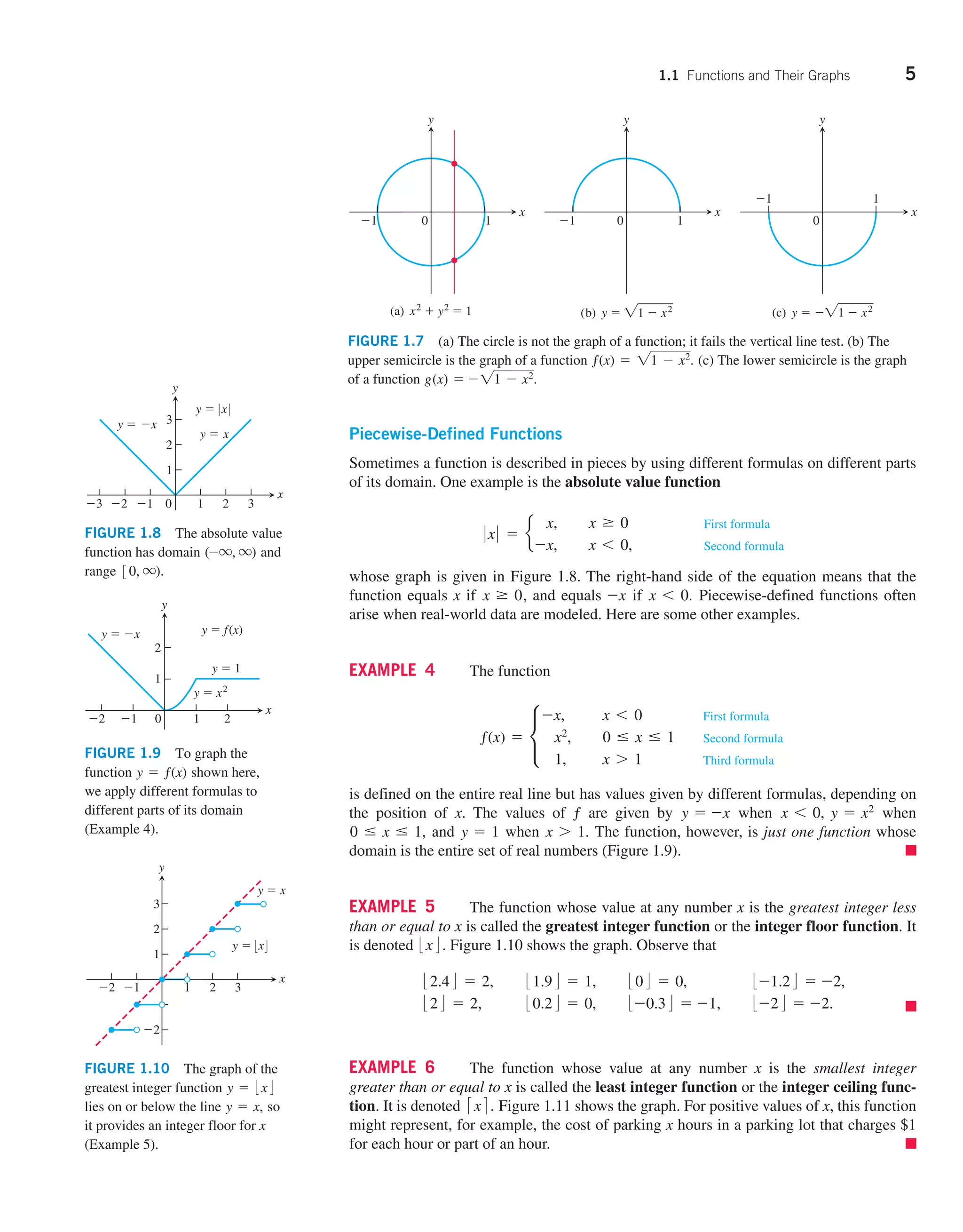
62. 48 Chapter 1: Functions
Domain:
Range:
x
y
1
−1
x = sin y
p
2
p
2
−
y = sin–1
x
−1 ≤ x ≤ 1
−p2 ≤ y ≤ p2
FIGURE 1.64 The graph of y = sin-1
x.
increases from -1 at x = -p2 to +1 at x = p2. By restricting its domain to the inter-
val 3-p2, p2] we make it one-to-one, so that it has an inverse sin-1
x (Figure 1.64).
Similar domain restrictions can be applied to all six trigonometric functions.
0
1
−1
p
2
−
p
2
csc x
x
y
0
1
p
p
2
sec x
x
y
−1
0 p p
2
cot x
x
y
tan x
x
y
0 p
2
p
2
−
0
−1
1
p p
2
cos x
x
y
x
y
0 p
2
p
2
−
sin x
−1
1
y = sin x
Domain: 3-p2, p24
Range: 3-1, 14
y = cos x
Domain: 30, p4
Range: 3-1, 14
y = tan x
Domain: (-p2, p2)
Range: (-q, q)
y = csc x
Domain: 3-p2, 0) ∪ (0, p24
Range: (-q, -14 ∪ 31, q)
y = cot x
Domain: (0, p)
Range: (-q, q)
y = sec x
Domain: 30, p2) ∪ (p2, p4
Range: (-q, -14 ∪ 31, q)
Domain restrictions that make the trigonometric functions one-to-one
Since these restricted functions are now one-to-one, they have inverses, which we
denote by
y = sin-1
x or y = arcsin x
y = cos-1
x or y = arccos x
y = tan-1
x or y = arctan x
y = cot-1
x or y = arccot x
y = sec-1
x or y = arcsec x
y = csc-1
x or y = arccsc x
These equations are read “y equals the arcsine of x” or “y equals arcsin x” and so on.
Caution The -1 in the expressions for the inverse means “inverse.” It does not mean
reciprocal. For example, the reciprocal of sin x is (sin x)-1
= 1sin x = csc x.
The graphs of the six inverse trigonometric functions are obtained by reflecting the
graphs of the restricted trigonometric functions through the line y = x. Figure 1.65b
shows the graph of y = sin-1
x and Figure 1.66 shows the graphs of all six functions. We
now take a closer look at two of these functions.
The Arcsine and Arccosine Functions
We define the arcsine and arccosine as functions whose values are angles (measured in
radians) that belong to restricted domains of the sine and cosine functions.
x
y
x
y
1
−1
0
0 1
−1
(a)
(b)
p
2
p
2
p
2
−
p
2
−
y = sin x, p
2
p
2
− ≤ x ≤
Domain:
Range:
[−p2, p2]
[−1, 1]
x = sin y
y = sin–1
x
Domain:
Range:
[−1, 1]
[−p2, p2]
FIGURE 1.65 The graphs of
(a) y = sin x, -p2 … x … p2, and
(b) its inverse, y = sin-1
x. The graph
of sin-1
x, obtained by reflection across
the line y = x, is a portion of the curve
x = sin y.

63. 1.6 Inverse Functions and Logarithms 49
The graph of y = sin-1
x (Figure 1.65b) is symmetric about the origin (it lies along the
graph of x = sin y). The arcsine is therefore an odd function:
sin-1
(-x) = -sin-1
x. (2)
The graph of y = cos-1
x (Figure 1.67b) has no such symmetry.
EXAMPLE 8 Evaluate (a) sin-1
a
23
2
b and (b) cos-1
a-
1
2
b .
Solution
(a) We see that
sin-1
a
23
2
b =
p
3
because sin(p3) = 232 and p3 belongs to the range 3-p2, p24 of the arc-
sine function. See Figure 1.68a.
(b) We have
cos-1
a-
1
2
b =
2p
3
because cos(2p3) = -12 and 2p3 belongs to the range 30, p4 of the arccosine
function. See Figure 1.68b.
x
y
p
2
p
2
−
1
−1
(a)
Domain:
Range:
−1 ≤ x ≤ 1
≤ y ≤
p
2
−
p
2
y = sin–1x
x
y
p
p
2
1
−1
Domain:
Range:
−1 ≤ x ≤ 1
0 ≤ y ≤ p
(b)
y = cos–1
x
x
y
(c)
Domain: −∞ x ∞
Range: y
p
2
−
p
2
1
−1
−2 2
p
2
p
2
−
y = tan–1
x
x
y
(d)
Domain:
Range:
x ≤ −1 or x ≥ 1
0 ≤ y ≤ p, y ≠
1
−1
−2 2
y = sec–1
x
p
p
2
p
2
x
y
Domain:
Range:
x ≤ −1 or x ≥ 1
≤ y ≤ , y ≠ 0
p
2
−
p
2
(e)
1
−1
−2 2
p
2
p
2
−
y = csc–1
x
x
y
Domain:
Range: 0 y p
(f)
p
p
2
1
−1
−2 2
y = cot–1
x
−∞ x ∞
FIGURE 1.66 Graphs of the six basic inverse trigonometric functions.
DEFINITION
y = sin−1
x is the number in 3-p2, p24 for which sin y = x.
y = cos−1
x is the number in 30, p4 for which cos y = x.
The “Arc” in Arcsine and Arccosine
For a unit circle and radian angles, the
arc length equation s = ru becomes
s = u, so central angles and the arcs
they subtend have the same measure.
If x = sin y, then, in addition to being
the angle whose sine is x, y is also the
length of arc on the unit circle that
subtends an angle whose sine is x. So
we call y “the arc whose sine is x.”
Arc whose sine is x
Arc whose
cosine is x
x2
+ y2
= 1
Angle whose
sine is x
Angle whose
cosine is x
x
y
0 x 1

64. 50 Chapter 1: Functions
Using the same procedure illustrated in Example 8, we can create the following table of
common values for the arcsine and arccosine functions.
x sin-1
x cos-1
x
232 p3 p6
222 p4 p4
12 p6 p3
-12 -p6 2p3
- 222 -p4 3p4
- 232 -p3 5p6
FIGURE 1.68 Values of the arcsine and arccosine functions
(Example 8).
x
y
p
3
0 1
2 3
p
3
sin = 3
2
p
3
sin–1
=
3
2
(a)
a b
0
−1
x
y
3
2
p
3
2
p
3
2
−
cos–1 1
2
=
p
3
2
cos = –1
2
(b)
a b
x
y
x
y
0 p p
2
y = cos x, 0 ≤ x ≤ p
Domain:
Range:
[0, p]
[−1, 1]
y = cos–1
x
Domain:
Range:
[−1, 1]
[0, p]
1
−1
(a)
(b)
p
p
2
0
−1 1
x = cos y
FIGURE 1.67 The graphs of (a) y = cos x,
0 … x … p, and (b) its inverse, y = cos-1
x.
The graph of cos-1
x, obtained by reflection
across the line y = x, is a portion of the curve
x = cos y.
EXAMPLE 9 During a 240 mi airplane flight from Chicago to St. Louis, after flying
180 mi the navigator determines that the plane is 12 mi off course, as shown in Figure
1.69. Find the angle a for a course parallel to the original correct course, the angle b, and
the drift correction angle c = a + b.
Solution From the Pythagorean theorem and given information, we compute an approxi-
mate hypothetical flight distance of 179 mi, had the plane been flying along the original
correct course (see Figure 1.69). Knowing the flight distance from Chicago to St. Louis, we
next calculate the remaining leg of the original course to be 61 mi. Applying the Pythagorean
theorem again then gives an approximate distance of 62 mi from the position of the plane to
St. Louis. Finally, from Figure 1.69, we see that 180 sin a = 12 and 62 sin b = 12, so
a = sin-1 12
180
≈ 0.067 radian ≈ 3.8°
b = sin-1 12
62
≈ 0.195 radian ≈ 11.2°
c = a + b ≈ 15°.
Identities Involving Arcsine and Arccosine
As we can see from Figure 1.70, the arccosine of x satisfies the identity
cos-1
x + cos-1
(-x) = p, (3)
or
cos-1
(-x) = p - cos-1
x. (4)
Also, we can see from the triangle in Figure 1.71 that for x 7 0,
sin-1
x + cos-1
x = p2. (5)
Chicago
Plane position
St. Louis
62
61 12
180
179
a
b
c
FIGURE 1.69 Diagram for drift correc-
tion (Example 9), with distances surrounded
to the nearest mile (drawing not to scale).
FIGURE 1.70 cos-1
x and cos-1
(-x) are
supplementary angles (so their sum is p).
x
y
0
−x x
−1 1
cos–1
x
cos–1
(−x)

65. 1.6 Inverse Functions and Logarithms 51
Equation (5) holds for the other values of x in 3-1, 1] as well, but we cannot conclude this
from the triangle in Figure 1.71. It is, however, a consequence of Equations (2) and (4)
(Exercise 76).
The arctangent, arccotangent, arcsecant, and arccosecant functions are defined in Sec-
tion 3.9. There we develop additional properties of the inverse trigonometric functions in a
calculus setting using the identities discussed here.
1
x
cos–1
x
sin–1
x
FIGURE 1.71 sin-1
x and cos-1
x are
complementary angles (so their sum is p2).
Identifying One-to-One Functions Graphically
Which of the functions graphed in Exercises 1–6 are one-to-one, and
which are not?
1.
x
y
0
y = −3x3
2.
x
y
0
−1 1
y = x4
− x2
3. y
x
y = 20 x 0
4. y
y = int x
5.
x
y
0
y = 1
x
6.
x
y
y = x13
In Exercises 7–10, determine from its graph if the function is one-to-
one.
7. ƒ(x) = e
3 - x, x 6 0
3, x Ú 0
8. ƒ(x) = e
2x + 6, x … -3
x + 4, x 7 -3
9. ƒ(x) = d
1 -
x
2
, x … 0
x
x + 2
, x 7 0
10. ƒ(x) = e
2 - x2
, x … 1
x2
, x 7 1
Graphing Inverse Functions
Each of Exercises 11–16 shows the graph of a function y = ƒ(x).
Copy the graph and draw in the line y = x. Then use symmetry with
respect to the line y = x to add the graph of ƒ-1
to your sketch. (It is
not necessary to find a formula for ƒ-1
.) Identify the domain and
range of ƒ-1
.
11. 12.
x
y
1
0
1
y = f(x) = , x ≥ 0
1
x2
+ 1
x
y
1
0
1
y = f(x) = 1 − , x 0
1
x
13. 14.
x
y
0 p
2
p
2
−
1
−1
p
2
p
2
−
y = f(x) = sin x,
≤ x ≤ p
2
p
2
−
y = f(x) = tan x,
x
x
y
0 p
2
p
2
−
15. 16.
x
y
0
6
3
f(x) = 6 − 2x,
0 ≤ x ≤ 3 x
y
0
1
−1 3
−2
x + 1, −1 ≤ x ≤ 0
−2 + x, 0 x 3
f(x) = 2
3
17. a. Graph the function ƒ(x) = 21 - x2
, 0 … x … 1. What sym-
metry does the graph have?
b. Show that ƒ is its own inverse. (Remember that 2x2
= x if
x Ú 0.)
18. a. Graph the function ƒ(x) = 1x. What symmetry does the
graph have?
b. Show that ƒ is its own inverse.
Exercises 1.6

66. 52 Chapter 1: Functions
Formulas for Inverse Functions
Each of Exercises 19–24 gives a formula for a function y = ƒ(x) and
shows the graphs of ƒ and ƒ-1
. Find a formula for ƒ-1
in each case.
19. ƒ(x) = x2
+ 1, x Ú 0 20. ƒ(x) = x2
, x … 0
x
y
1
1
0
y = f(x)
y = f –1
(x)
x
y
1
1
0
y = f –1
(x)
y = f(x)
21. ƒ(x) = x3
- 1 22. ƒ(x) = x2
- 2x + 1, x Ú 1
x
y
1
1
−1
−1
y = f(x)
y = f –1
(x)
x
y
1
1
0
y = f(x)
y = f –1
(x)
23. ƒ(x) = (x + 1)2
, x Ú -1 24. ƒ(x) = x23
, x Ú 0
x
y
0
1
−1
1
−1
y = f(x)
y = f –1
(x)
x
y
0
1
1
y = f –1
(x)
y = f(x)
Each of Exercises 25–36 gives a formula for a function y = ƒ(x). In
each case, find ƒ-1
(x) and identify the domain and range of ƒ-1
. As a
check, show that ƒ(ƒ-1
(x)) = ƒ-1
(ƒ(x)) = x.
25. ƒ(x) = x5
26. ƒ(x) = x4
, x Ú 0
27. ƒ(x) = x3
+ 1 28. ƒ(x) = (12)x - 72
29. ƒ(x) = 1x2
, x 7 0 30. ƒ(x) = 1x3
, x ≠ 0
31. ƒ(x) =
x + 3
x - 2
32. ƒ(x) =
2x
2x - 3
33. ƒ(x) = x2
- 2x, x … 1 34. ƒ(x) = (2x3
+ 1)15
(Hint: Complete the square.)
35. ƒ(x) =
x + b
x - 2
, b 7 -2 and constant
36. ƒ(x) = x2
- 2bx, b 7 0 and constant, x … b
Inverses of Lines
37. a. Find the inverse of the function ƒ(x) = mx, where m is a con-
stant different from zero.
b. What can you conclude about the inverse of a function
y = ƒ(x) whose graph is a line through the origin with a non-
zero slope m?
38. Show that the graph of the inverse of ƒ(x) = mx + b, where m
and b are constants and m ≠ 0, is a line with slope 1m and
y-intercept -bm.
39. a. Find the inverse of ƒ(x) = x + 1. Graph ƒ and its inverse
together. Add the line y = x to your sketch, drawing it with
dashes or dots for contrast.
b. Find the inverse of ƒ(x) = x + b (b constant). How is the
graph of ƒ-1
related to the graph of ƒ?
c. What can you conclude about the inverses of functions whose
graphs are lines parallel to the line y = x?
40. a. Find the inverse of ƒ(x) = -x + 1. Graph the line
y = -x + 1 together with the line y = x. At what angle do
the lines intersect?
b. Find the inverse of ƒ(x) = -x + b (b constant). What angle
does the line y = -x + b make with the line y = x?
c. What can you conclude about the inverses of functions whose
graphs are lines perpendicular to the line y = x?
Logarithms and Exponentials
41. Express the following logarithms in terms of ln 2 and ln 3.
a. ln 0.75 b. ln (49)
c. ln (12) d. ln2
3
9
e. ln322 f. ln 213.5
42. Express the following logarithms in terms of ln 5 and ln 7.
a. ln (1125) b. ln 9.8
c. ln727 d. ln 1225
e. ln 0.056 f. (ln35 + ln(17))(ln25)
Use the properties of logarithms to write the expressions in Exercises
43 and 44 as a single term.
43. a. lnsin u - ln a
sin u
5
b b. ln(3x2
- 9x) + ln a
1
3x
b
c.
1
2
ln(4t4
) - lnb
44. a. lnsec u + lncos u b. ln(8x + 4) - 2lnc
c. 3ln2
3
t2
- 1 - ln(t + 1)
Find simpler expressions for the quantities in Exercises 45–48.
45. a. eln7.2
b. e-lnx2
c. elnx-lny
46. a. eln(x2
+y2
)
b. e-ln0.3
c. elnpx-ln2
47. a. 2ln 2e b. ln(lnee
) c. ln(e-x2
-y2
)
48. a. ln(esec u
) b. ln(e(ex
)
) c. ln(e2lnx
)
In Exercises 49–54, solve for y in terms of t or x, as appropriate.
49. lny = 2t + 4 50. lny = -t + 5
51. ln(y - b) = 5t 52. ln(c - 2y) = t
53. ln(y - 1) - ln2 = x + lnx
54. ln(y2
- 1) - ln(y + 1) = ln(sin x)

67. 1.6 Inverse Functions and Logarithms 53
In Exercises 55 and 56, solve for k.
55. a. e2k
= 4 b. 100e10k
= 200 c. ek1000
= a
56. a. e5k
=
1
4
b. 80ek
= 1 c. e(ln0.8)k
= 0.8
In Exercises 57–60, solve for t.
57. a. e-0.3t
= 27 b. ekt
=
1
2
c. e(ln0.2)t
= 0.4
58. a. e-0.01t
= 1000 b. ekt
=
1
10
c. e(ln2)t
=
1
2
59. e2t
= x2
60. e(x2
)
e(2x+1)
= et
Simplify the expressions in Exercises 61–64.
61. a. 5log5 7
b. 8log822
c. 1.3log1.3 75
d. log4 16 e. log323 f. log4 a
1
4
b
62. a. 2log2 3
b. 10log10 (12)
c. plogp 7
d. log11 121 e. log121 11 f. log3 a
1
9
b
63. a. 2log4 x
b. 9log3 x
c. log2(e(ln2)(sin x)
)
64. a. 25log5 (3x2
)
b. loge(ex
) c. log4(2ex
sin x
)
Express the ratios in Exercises 65 and 66 as ratios of natural loga-
rithms and simplify.
65. a.
log2 x
log3 x
b.
log2 x
log8 x
c.
logx a
logx2 a
66. a.
log9 x
log3 x
b.
log210 x
log22 x
c.
loga b
logb a
Arcsine and Arccosine
In Exercises 67–70, find the exact value of each expression.
67. a. sin-1
a
-1
2
b b. sin-1
a
1
22
b c. sin-1
a
- 23
2
b
68. a. cos-1
a
1
2
b b. cos-1
a
-1
22
b c. cos-1
a
23
2
b
69. a. arccos (-1) b. arccos (0)
70. a. arcsin (-1) b. arcsin a-
1
22
b
Theory and Examples
71. If ƒ(x) is one-to-one, can anything be said about g(x) = -ƒ(x)? Is
it also one-to-one? Give reasons for your answer.
72. If ƒ(x) is one-to-one and ƒ(x) is never zero, can anything be said
about h(x) = 1ƒ(x)? Is it also one-to-one? Give reasons for your
answer.
73. Suppose that the range of g lies in the domain of ƒ so that the
composite ƒ ∘ g is defined. If ƒ and g are one-to-one, can any-
thing be said about ƒ ∘ g? Give reasons for your answer.
74. If a composite ƒ ∘ g is one-to-one, must g be one-to-one? Give
reasons for your answer.
75. Find a formula for the inverse function ƒ-1
and verify that
(ƒ ∘ ƒ-1
)(x) = (ƒ-1
∘ ƒ)(x) = x.
a. ƒ(x) =
100
1 + 2-x b. ƒ(x) =
50
1 + 1.1-x
76. The identity sin-1
x + cos-1
x = P2 Figure 1.71 establishes
the identity for 0 6 x 6 1. To establish it for the rest of 3-1, 1],
verify by direct calculation that it holds for x = 1, 0, and -1.
Then, for values of x in (-1, 0), let x = -a, a 7 0, and apply
Eqs. (3) and (5) to the sum sin-1
(-a) + cos-1
(-a).
77. Start with the graph of y = lnx. Find an equation of the graph
that results from
a. shifting down 3 units.
b. shifting right 1 unit.
c. shifting left 1, up 3 units.
d. shifting down 4, right 2 units.
e. reflecting about the y-axis.
f. reflecting about the line y = x.
78. Start with the graph of y = lnx. Find an equation of the graph
that results from
a. vertical stretching by a factor of 2.
b. horizontal stretching by a factor of 3.
c. vertical compression by a factor of 4.
d. horizontal compression by a factor of 2.
79. The equation x2
= 2x
has three solutions: x = 2, x = 4, and one
other. Estimate the third solution as accurately as you can by
graphing.
80. Could xln 2
possibly be the same as 2ln x
for x 7 0? Graph the
two functions and explain what you see.
81. Radioactive decay The half-life of a certain radioactive sub-
stance is 12 hours. There are 8 grams present initially.
a. Express the amount of substance remaining as a function of
time t.
b. When will there be 1 gram remaining?
82. Doubling your money Determine how much time is required
for a $500 investment to double in value if interest is earned at the
rate of 4.75% compounded annually.
83. Population growth The population of Glenbrook is 375,000
and is increasing at the rate of 2.25% per year. Predict when the
population will be 1 million.
84. Radon-222 The decay equation for radon-222 gas is known to
be y = y0e-0.18t
, with t in days. About how long will it take the
radon in a sealed sample of air to fall to 90% of its original value?
T
T

68. 54 Chapter 1: Functions
Chapter 1 Questions to Guide Your Review
1. What is a function? What is its domain? Its range? What is an
arrow diagram for a function? Give examples.
2. What is the graph of a real-valued function of a real variable?
What is the vertical line test?
3. What is a piecewise-defined function? Give examples.
4. What are the important types of functions frequently encountered
in calculus? Give an example of each type.
5. What is meant by an increasing function? A decreasing function?
Give an example of each.
6. What is an even function? An odd function? What symmetry
properties do the graphs of such functions have? What advantage
can we take of this? Give an example of a function that is neither
even nor odd.
7. If ƒ and g are real-valued functions, how are the domains of
ƒ + g, ƒ - g, ƒg, and ƒg related to the domains of ƒ and g?
Give examples.
8. When is it possible to compose one function with another? Give
examples of composites and their values at various points. Does
the order in which functions are composed ever matter?
9. How do you change the equation y = ƒ(x) to shift its graph verti-
cally up or down by k units? Horizontally to the left or right?
Give examples.
10. How do you change the equation y = ƒ(x) to compress or stretch
the graph by a factor c 7 1? Reflect the graph across a coordi-
nate axis? Give examples.
11. What is radian measure? How do you convert from radians to
degrees? Degrees to radians?
12. Graph the six basic trigonometric functions. What symmetries do
the graphs have?
13. What is a periodic function? Give examples. What are the periods
of the six basic trigonometric functions?
14. Starting with the identity sin2
u + cos2
u = 1 and the formulas
for cos (A + B) and sin (A + B), show how a variety of other
trigonometric identities may be derived.
15. How does the formula for the general sine function ƒ(x) =
Asin ((2pB)(x - C)) + D relate to the shifting, stretching,
compressing, and reflection of its graph? Give examples.
Graph the general sine curve and identify the constants A, B,
C, and D.
16. Name three issues that arise when functions are graphed using a
calculator or computer with graphing software. Give examples.
17. What is an exponential function? Give examples. What laws of
exponents does it obey? How does it differ from a simple power
function like ƒ(x) = xn
? What kind of real-world phenomena are
modeled by exponential functions?
18. What is the number e, and how is it defined? What are the domain
and range of ƒ(x) = ex
? What does its graph look like? How do
the values of ex
relate to x2
, x3
, and so on?
19. What functions have inverses? How do you know if two func-
tions ƒ and g are inverses of one another? Give examples of func-
tions that are (are not) inverses of one another.
20. How are the domains, ranges, and graphs of functions and their
inverses related? Give an example.
21. What procedure can you sometimes use to express the inverse of
a function of x as a function of x?
22. What is a logarithmic function? What properties does it satisfy?
What is the natural logarithm function? What are the domain and
range of y = ln x? What does its graph look like?
23. How is the graph of loga x related to the graph of ln x? What truth
is in the statement that there is really only one exponential func-
tion and one logarithmic function?
24. How are the inverse trigonometric functions defined? How can
you sometimes use right triangles to find values of these func-
tions? Give examples.
Chapter 1 Practice Exercises
Functions and Graphs
1. Express the area and circumference of a circle as functions of the
circle’s radius. Then express the area as a function of the
circumference.
2. Express the radius of a sphere as a function of the sphere’s sur-
face area. Then express the surface area as a function of the
volume.
3. A point P in the first quadrant lies on the parabola y = x2
.
Express the coordinates of P as functions of the angle of inclina-
tion of the line joining P to the origin.
4. A hot-air balloon rising straight up from a level field is tracked by
a range finder located 500 ft from the point of liftoff. Express the
balloon’s height as a function of the angle the line from the range
finder to the balloon makes with the ground.
In Exercises 5–8, determine whether the graph of the function is sym-
metric about the y-axis, the origin, or neither.
5. y = x15
6. y = x25
7. y = x2
- 2x - 1 8. y = e-x2

69. Chapter 1 Practice Exercises 55
In Exercises 9–16, determine whether the function is even, odd, or
neither.
9. y = x2
+ 1 10. y = x5
- x3
- x
11. y = 1 - cos x 12. y = sec x tan x
13. y =
x4
+ 1
x3
- 2x
14. y = x - sin x
15. y = x + cos x 16. y = x cos x
17. Suppose that ƒ and g are both odd functions defined on the entire
real line. Which of the following (where defined) are even? odd?
a. ƒg b. ƒ3
c. ƒ(sin x) d. g(sec x) e. 0 g0
18. If ƒ(a - x) = ƒ(a + x), show that g(x) = ƒ(x + a) is an even
function.
In Exercises 19–28, find the (a) domain and (b) range.
19. y = x - 2 20. y = -2 + 21 - x
21. y = 216 - x2
22. y = 32-x
+ 1
23. y = 2e-x
- 3 24. y = tan (2x - p)
25. y = 2sin (3x + p) - 1 26. y = x25
27. y = ln(x - 3) + 1 28. y = -1 + 2
3
2 - x
29. State whether each function is increasing, decreasing, or neither.
a. Volume of a sphere as a function of its radius
b. Greatest integer function
c. Height above Earth’s sea level as a function of atmospheric
pressure (assumed nonzero)
d. Kinetic energy as a function of a particle’s velocity
30. Find the largest interval on which the given function is increasing.
a. ƒ(x) = 0 x - 20 + 1 b. ƒ(x) = (x + 1)4
c. g(x) = (3x - 1)13
d. R(x) = 22x - 1
Piecewise-Defined Functions
In Exercises 31 and 32, find the (a) domain and (b) range.
31. y = e
2-x, -4 … x … 0
2x, 0 6 x … 4
32. y = c
-x - 2, -2 … x … -1
x, -1 6 x … 1
-x + 2, 1 6 x … 2
In Exercises 33 and 34, write a piecewise formula for the function.
33.
x
1
1
0 2
y 34.
x
5
(2, 5)
0 4
y
Composition of Functions
In Exercises 35 and 36, find
a. (ƒ ∘ g)(-1). b. (g ∘ ƒ)(2).
c. (ƒ ∘ ƒ)(x). d. (g ∘ g)(x).
35. ƒ(x) =
1
x, g(x) =
1
2x + 2
36. ƒ(x) = 2 - x, g(x) = 2
3
x + 1
In Exercises 37 and 38, (a) write formulas for ƒ ∘ g and g ∘ ƒ and find
the (b) domain and (c) range of each.
37. ƒ(x) = 2 - x2
, g(x) = 2x + 2
38. ƒ(x) = 2x, g(x) = 21 - x
For Exercises 39 and 40, sketch the graphs of ƒ and ƒ ∘ ƒ.
39. ƒ(x) = c
-x - 2, -4 … x … -1
-1, -1 6 x … 1
x - 2, 1 6 x … 2
40. ƒ(x) = b
x + 1, -2 … x 6 0
x - 1, 0 … x … 2
Composition with absolute values In Exercises 41–48, graph ƒ1
and ƒ2 together. Then describe how applying the absolute value func-
tion in ƒ2 affects the graph of ƒ1.
ƒ1(x) ƒ2(x)
41. x 0 x0
42. x2 0 x0 2
43. x3 0 x3 0
44. x2
+ x 0 x2
+ x0
45. 4 - x2 0 4 - x2 0
46.
1
x
1
0 x0
47. 2x 2 0 x0
48. sin x sin 0 x0
Shifting and Scaling Graphs
49. Suppose the graph of g is given. Write equations for the graphs
that are obtained from the graph of g by shifting, scaling, or
reflecting, as indicated.
a. Up
1
2
unit, right 3
b. Down 2 units, left
2
3
c. Reflect about the y-axis
d. Reflect about the x-axis
e. Stretch vertically by a factor of 5
f. Compress horizontally by a factor of 5
50. Describe how each graph is obtained from the graph of y = ƒ(x).
a. y = ƒ(x - 5) b. y = ƒ(4x)
c. y = ƒ(-3x) d. y = ƒ(2x + 1)
e. y = ƒa
x
3
b - 4 f. y = -3ƒ(x) +
1
4

70. 56 Chapter 1: Functions
In Exercises 51–54, graph each function, not by plotting points, but by
starting with the graph of one of the standard functions presented in
Figures 1.15–1.17, and applying an appropriate transformation.
51. y = -
A
1 +
x
2
52. y = 1 -
x
3
53. y =
1
2x2
+ 1 54. y = (-5x)13
Trigonometry
In Exercises 55–58, sketch the graph of the given function. What is
the period of the function?
55. y = cos 2x 56. y = sin
x
2
57. y = sin px 58. y = cos
px
2
59. Sketch the graph y = 2cos ax -
p
3
b .
60. Sketch the graph y = 1 + sin ax +
p
4
b .
In Exercises 61–64, ABC is a right triangle with the right angle at C.
The sides opposite angles A, B, and C are a, b, and c, respectively.
61. a. Find a and b if c = 2, B = p3.
b. Find a and c if b = 2, B = p3.
62. a. Express a in terms of A and c.
b. Express a in terms of A and b.
63. a. Express a in terms of B and b.
b. Express c in terms of A and a.
64. a. Express sin A in terms of a and c.
b. Express sin A in terms of b and c.
65. Height of a pole Two wires stretch from the top T of a vertical
pole to points B and C on the ground, where C is 10 m closer to
the base of the pole than is B. If wire BT makes an angle of 35°
with the horizontal and wire CT makes an angle of 50° with the
horizontal, how high is the pole?
66. Height of a weather balloon Observers at positions A and B
2 km apart simultaneously measure the angle of elevation of a
weather balloon to be 40° and 70°, respectively. If the balloon is
directly above a point on the line segment between A and B, find
the height of the balloon.
67. a. Graph the function ƒ(x) = sin x + cos(x2).
b. What appears to be the period of this function?
c. Confirm your finding in part (b) algebraically.
68. a. Graph ƒ(x) = sin (1x).
b. What are the domain and range of ƒ?
c. Is ƒ periodic? Give reasons for your answer.
T
T
Transcendental Functions
In Exercises 69–72, find the domain of each function.
69. a. ƒ(x) = 1 + e-sin x
b. g(x) = ex
+ ln 2x
70. a. ƒ(x) = e1x2
b. g(x) = ln0 4 - x2 0
71. a. h(x) = sin-1
a
x
3
b b. ƒ(x) = cos-1
(2x - 1)
72. a. h(x) = ln (cos-1
x) b. ƒ(x) = 2p - sin-1
x
73. If ƒ(x) = lnx and g(x) = 4 - x2
, find the functions
ƒ ∘ g, g ∘ ƒ, ƒ ∘ ƒ, g ∘ g, and their domains.
74. Determine whether ƒ is even, odd, or neither.
a. ƒ(x) = e-x2
b. ƒ(x) = 1 + sin-1
(-x)
c. ƒ(x) = 0 ex 0 d. ƒ(x) = eln x +1
75. Graph ln x, ln 2x, ln 4x, ln 8x, and ln 16x (as many as you can)
together for 0 6 x … 10. What is going on? Explain.
76. Graph y = ln(x2
+ c) for c = -4, -2, 0, 3, and 5. How does the
graph change when c changes?
77. Graph y = ln sin x in the window 0 … x … 22, -2 … y … 0.
Explain what you see. How could you change the formula to turn
the arches upside down?
78. Graph the three functions y = xa
, y = ax
, and y = loga x to-
gether on the same screen for a = 2, 10, and 20. For large values
of x, which of these functions has the largest values and which
has the smallest values?
Theory and Examples
In Exercises 79 and 80, find the domain and range of each composite
function. Then graph the composites on separate screens. Do the
graphs make sense in each case? Give reasons for your answers and
comment on any differences you see.
79. a. y = sin-1
(sin x) b. y = sin (sin-1
x)
80. a. y = cos-1
(cos x) b. y = cos (cos-1
x)
81. Use a graph to decide whether ƒ is one-to-one.
a. ƒ(x) = x3
-
x
2
b. ƒ(x) = x3
+
x
2
82. Use a graph to find to 3 decimal places the values of x for which
ex
7 10,000,000.
83. a. Show that ƒ(x) = x3
and g(x) = 2
3
x are inverses of one
another.
b. Graph ƒ and g over an x-interval large enough to show the
graphs intersecting at (1, 1) and (-1, -1). Be sure the picture
shows the required symmetry in the line y = x.
84. a. Show that h(x) = x3
4 and k(x) = (4x)13
are inverses of one
another.
b. Graph h and k over an x-interval large enough to show the
graphs intersecting at (2, 2) and (-2, -2). Be sure the picture
shows the required symmetry in the line y = x.
T
T
T
T
T
T
T

71. Chapter 1 Additional and Advanced Exercises 57
Chapter 1 Additional and Advanced Exercises
Functions and Graphs
1. Are there two functions ƒ and g such that ƒ ∘ g = g ∘ ƒ? Give
reasons for your answer.
2. Are there two functions ƒ and g with the following property? The
graphs of ƒ and g are not straight lines but the graph of ƒ ∘ g is a
straight line. Give reasons for your answer.
3. If ƒ(x) is odd, can anything be said of g(x) = ƒ(x) - 2? What if ƒ
is even instead? Give reasons for your answer.
4. If g(x) is an odd function defined for all values of x, can anything
be said about g(0)? Give reasons for your answer.
5. Graph the equation 0 x0 + 0 y0 = 1 + x.
6. Graph the equation y + y = x + x.
Derivations and Proofs
7. Prove the following identities.
a.
1 - cos x
sin x
=
sin x
1 + cos x
b.
1 - cos x
1 + cos x
= tan2 x
2
8. Explain the following “proof without words” of the law of cosines.
(Source: Kung, Sidney H., “Proof Without Words: The Law of
Cosines,” Mathematics Magazine, Vol. 63, no. 5, Dec. 1990, p. 342.)
a a
a
c b
a − c
2a cos u − b
u
9. Show that the area of triangle ABC is given by
(12)absin C = (12)bc sin A = (12)ca sin B.
B
A
C
a
b
c
10. Show that the area of triangle ABC is given by
2s(s - a)(s - b)(s - c) where s = (a + b + c)2 is the
semiperimeter of the triangle.
11. Show that if ƒ is both even and odd, then ƒ(x) = 0 for every x in
the domain of ƒ.
12. a. Even-odd decompositions Let ƒ be a function whose
domain is symmetric about the origin, that is, -x belongs to
the domain whenever x does. Show that ƒ is the sum of an
even function and an odd function:
ƒ(x) = E(x) + O(x),
where E is an even function and O is an odd function. (Hint:
Let E(x) = (ƒ(x) + ƒ(-x))2. Show that E(-x) = E(x), so
that E is even. Then show that O(x) = ƒ(x) - E(x) is odd.)
b. Uniqueness Show that there is only one way to write ƒ as
the sum of an even and an odd function. (Hint: One way is
given in part (a). If also ƒ(x) = E1(x) + O1(x) where E1 is
even and O1 is odd, show that E - E1 = O1 - O. Then use
Exercise 11 to show that E = E1 and O = O1.)
Effects of Parameters on Graphs
13. What happens to the graph of y = ax2
+ bx + c as
a. a changes while b and c remain fixed?
b. b changes (a and c fixed, a ≠ 0)?
c. c changes (a and b fixed, a ≠ 0)?
14. What happens to the graph of y = a(x + b)3
+ c as
a. a changes while b and c remain fixed?
b. b changes (a and c fixed, a ≠ 0)?
c. c changes (a and b fixed, a ≠ 0)?
Geometry
15. An object’s center of mass moves at a constant velocity y along a
straight line past the origin. The accompanying figure shows the
coordinate system and the line of motion. The dots show posi-
tions that are 1 sec apart. Why are the areas A1, A2, c, A5 in the
figure all equal? As in Kepler’s equal area law (see Section 13.6),
the line that joins the object’s center of mass to the origin sweeps
out equal areas in equal times.
x
y
0 5 10 15
Kilometers
5
10
Kilometers
A5
A4
A3
A2
A1
t = 6
t = 5
t = 1
t = 2
yΔt
yΔt
16. a. Find the slope of the line from the origin to the midpoint P of
side AB in the triangle in the accompanying figure (a, b 7 0).
x
y
P
B(0, b)
A(a, 0)
O
b. When is OP perpendicular to AB?
T
T

72. 58 Chapter 1: Functions
17. Consider the quarter-circle of radius 1 and right triangles ABE
and ACD given in the accompanying figure. Use standard area
formulas to conclude that
1
2
sin u cos u 6
u
2
6
1
2
sin u
cos u
.
x
y
B
E
C
(0, 1)
A (1, 0)
D
1
u
18. Let ƒ(x) = ax + b and g(x) = cx + d. What condition must be
satisfied by the constants a, b, c, d in order that (ƒ ∘ g)(x) =
(g ∘ ƒ)(x) for every value of x?
Theory and Examples
19. Domain and range Suppose that a ≠ 0, b ≠ 1, and b 7 0.
Determine the domain and range of the function.
a. y = a(bc-x
) + d b. y = a logb(x - c) + d
20. Inverse functions Let
ƒ(x) =
ax + b
cx + d
, c ≠ 0, ad - bc ≠ 0.
a. Give a convincing argument that ƒ is one-to-one.
b. Find a formula for the inverse of ƒ.
21. Depreciation Smith Hauling purchased an 18-wheel truck for
$100,000. The truck depreciates at the constant rate of $10,000
per year for 10 years.
a. Write an expression that gives the value y after x years.
b. When is the value of the truck $55,000?
22. Drug absorption A drug is administered intravenously for
pain. The function
ƒ(t) = 90 - 52 ln (1 + t), 0 … t … 4
gives the number of units of the drug remaining in the body after t
hours.
a. What was the initial number of units of the drug administered?
b. How much is present after 2 hours?
c. Draw the graph of ƒ.
23. Finding investment time If Juanita invests $1500 in a retire-
ment account that earns 8% compounded annually, how long will
it take this single payment to grow to $5000?
24. The rule of 70 If you use the approximation ln 2 ≈ 0.70 (in
place of 0.69314c), you can derive a rule of thumb that says,
“To estimate how many years it will take an amount of money to
double when invested at r percent compounded continuously,
divide r into 70.” For instance, an amount of money invested at
5% will double in about 705 = 14 years. If you want it to dou-
ble in 10 years instead, you have to invest it at 7010 = 7%.
Show how the rule of 70 is derived. (A similar “rule of 72” uses
72 instead of 70, because 72 has more integer factors.)
25. For what x 7 0 does x(xx
)
= (xx
)x
? Give reasons for your answer.
26. a. If (lnx)x = (ln2)2, must x = 2?
b. If (lnx)x = -2ln2, must x = 12?
Give reasons for your answers.
27. The quotient (log4 x)(log2 x) has a constant value. What value?
Give reasons for your answer.
28. logx (2) vs. log2 (x) How does ƒ(x) = logx (2) compare with
g(x) = log2 (x)? Here is one way to find out.
a. Use the equation loga b = (lnb)(lna) to express ƒ(x) and
g(x) in terms of natural logarithms.
b. Graph ƒ and g together. Comment on the behavior of ƒ in
relation to the signs and values of g.
T
T
Chapter 1 Technology Application Projects
An Overview of Mathematica
An overview of Mathematica sufficient to complete the Mathematica modules appearing on the Web site.
Mathematica/Maple Module:
Modeling Change: Springs, Driving Safety, Radioactivity, Trees, Fish, and Mammals
Construct and interpret mathematical models, analyze and improve them, and make predictions using them.

73. 59
Overview Mathematicians of the seventeenth century were keenly interested in the
study of motion for objects on or near the earth and the motion of planets and stars. This
study involved both the speed of the object and its direction of motion at any instant, and
they knew the direction at a given instant was along a line tangent to the path of motion.
The concept of a limit is fundamental to finding the velocity of a moving object and the
tangent to a curve. In this chapter we develop the limit, first intuitively and then formally.
We use limits to describe the way a function varies. Some functions vary continuously;
small changes in x produce only small changes in ƒ(x). Other functions can have values
that jump, vary erratically, or tend to increase or decrease without bound. The notion of
limit gives a precise way to distinguish between these behaviors.
2.1 Rates of Change and Tangents to Curves
Calculus is a tool that helps us understand how a change in one quantity is related to a
change in another. How does the speed of a falling object change as a function of time?
How does the level of water in a barrel change as a function of the amount of liquid poured
into it? We see change occurring in nearly everything we observe in the world and universe,
and powerful modern instruments help us see more and more. In this section we introduce
the ideas of average and instantaneous rates of change, and show that they are closely
related to the slope of a curve at a point P on the curve. We give precise developments of
these important concepts in the next chapter, but for now we use an informal approach so
you will see how they lead naturally to the main idea of this chapter, the limit. The idea of
a limit plays a foundational role throughout calculus.
Average and Instantaneous Speed
In the late sixteenth century, Galileo discovered that a solid object dropped from rest (not
moving) near the surface of the earth and allowed to fall freely will fall a distance proportional
to the square of the time it has been falling. This type of motion is called free fall. It assumes
negligible air resistance to slow the object down, and that gravity is the only force acting on
the falling object. If y denotes the distance fallen in feet after t seconds, then Galileo’s law is
y = 16t2
,
where 16 is the (approximate) constant of proportionality. (If y is measured in meters, the
constant is 4.9.)
A moving object’s average speed during an interval of time is found by dividing the
distance covered by the time elapsed. The unit of measure is length per unit time: kilome-
ters per hour, feet (or meters) per second, or whatever is appropriate to the problem at hand.
Limits and Continuity
2
HISTORICAL BIOGRAPHY*
Galileo Galilei
(1564–1642)
*To learn more about the historical figures mentioned in the text and the development of many major
elements and topics of calculus, visit www.aw.com/thomas.

74. 60 Chapter 2: Limits and Continuity
Example 1 A rock breaks loose from the top of a tall cliff. What is its average speed
(a) during the first 2 sec of fall?
(b) during the 1-sec interval between second 1 and second 2?
Solution The average speed of the rock during a given time interval is the change in
distance, ∆y, divided by the length of the time interval, ∆t. (Increments like ∆y and ∆t
are reviewed in Appendix 3, and pronounced “delta y” and “delta t.”) Measuring distance
in feet and time in seconds, we have the following calculations:
(a) For the first 2 sec:
∆y
∆t
=
16(2)2
- 16(0)2
2 - 0
= 32
ft
sec
(b) From sec 1 to sec 2:
∆y
∆t
=
16(2)2
- 16(1)2
2 - 1
= 48
ft
sec
We want a way to determine the speed of a falling object at a single instant t0, instead of
using its average speed over an interval of time. To do this, we examine what happens
when we calculate the average speed over shorter and shorter time intervals starting at t0.
The next example illustrates this process. Our discussion is informal here, but it will be
made precise in Chapter 3.
Example 2 Find the speed of the falling rock in Example 1 at t = 1 and t = 2sec.
Solution We can calculate the average speed of the rock over a time interval 3t0, t0 + h4,
having length ∆t = h, as
∆y
∆t
=
16(t0 + h)2
- 16t0
2
h
. (1)
We cannot use this formula to calculate the “instantaneous” speed at the exact moment t0
by simply substituting h = 0, because we cannot divide by zero. But we can use it to cal-
culate average speeds over increasingly short time intervals starting at t0 = 1 and t0 = 2.
When we do so, by taking smaller and smaller values of h, we see a pattern (Table 2.1).
Table 2.1 Average speeds over short time intervals 3t0, t0 + h4
Average speed:
∆y
∆t
=
16(t0 + h)2
- 16t0
2
h
Length of Average speed over Average speed over
time interval interval of length h interval of length h
h starting at t0 = 1 starting at t0 = 2
1 48 80
0.1 33.6 65.6
0.01 32.16 64.16
0.001 32.016 64.016
0.0001 32.0016 64.0016
The average speed on intervals starting at t0 = 1 seems to approach a limiting value
of 32 as the length of the interval decreases. This suggests that the rock is falling at a speed
of 32 ftsec at t0 = 1sec. Let’s confirm this algebraically.

75. 2.1 Rates of Change and Tangents to Curves 61
If we set t0 = 1 and then expand the numerator in Equation (1) and simplify, we find
that
∆y
∆t
=
16(1 + h)2
- 16(1)2
h
=
16(1 + 2h + h2
) - 16
h
=
32h + 16h2
h
= 32 + 16h.
For values of h different from 0, the expressions on the right and left are equivalent and the
average speed is 32 + 16h ftsec. We can now see why the average speed has the limiting
value 32 + 16(0) = 32 ftsec as h approaches 0.
Similarly, setting t0 = 2 in Equation (1), the procedure yields
∆y
∆t
= 64 + 16h
for values of h different from 0. As h gets closer and closer to 0, the average speed has the
limiting value 64 ftsec when t0 = 2sec, as suggested by Table 2.1.
The average speed of a falling object is an example of a more general idea which we
discuss next.
Average Rates of Change and Secant Lines
Given any function y = ƒ(x), we calculate the average rate of change of y with respect to
x over the interval [x1, x2] by dividing the change in the value of y, ∆y = ƒ(x2) - ƒ(x1),
by the length ∆x = x2 - x1 = h of the interval over which the change occurs. (We use
the symbol h for ∆x to simplify the notation here and later on.)
DEFINITION The average rate of change of y = ƒ(x) with respect to x over the
interval [x1, x2] is
∆y
∆x
=
ƒ(x2) - ƒ(x1)
x2 - x1
=
ƒ(x1 + h) - ƒ(x1)
h
, h ≠ 0.
Geometrically, the rate of change of ƒ over [x1, x2] is the slope of the line through the
points P(x1, ƒ(x1)) and Q(x2, ƒ(x2)) (Figure 2.1). In geometry, a line joining two points of a
curve is a secant to the curve. Thus, the average rate of change of ƒ from x1 to x2 is identi-
cal with the slope of secant PQ. Let’s consider what happens as the point Q approaches the
point P along the curve, so the length h of the interval over which the change occurs
approaches zero. We will see that this procedure leads to defining the slope of a curve at a
point.
Defining the Slope of a Curve
We know what is meant by the slope of a straight line, which tells us the rate at which it
rises or falls—its rate of change as a linear function. But what is meant by the slope of a
curve at a point P on the curve? If there is a tangent line to the curve at P—a line that just
touches the curve like the tangent to a circle—it would be reasonable to identify the slope
of the tangent as the slope of the curve at P. So we need a precise meaning for the tangent
at a point on a curve.
For circles, tangency is straightforward. A line L is tangent to a circle at a point P if L
passes through P perpendicular to the radius at P (Figure 2.2). Such a line just touches the
circle. But what does it mean to say that a line L is tangent to some other curve C at a point P?
P
L
O
Figure 2.2 L is tangent to the
circle at P if it passes through P
perpendicular to radius OP.
Figure 2.1 A secant to the graph
y = ƒ(x). Its slope is ∆y∆x, the
average rate of change of ƒ over the
interval [x1, x2].
y
x
0
Secant
P(x1, f(x1))
Q(x2, f(x2))
Δx = h
Δy
x2
x1
y = f(x)

76. 62 Chapter 2: Limits and Continuity
To define tangency for general curves, we need an approach that takes into account
the behavior of the secants through P and nearby points Q as Q moves toward P along the
curve (Figure 2.3). Here is the idea:
1. Start with what we can calculate, namely the slope of the secant PQ.
2. Investigate the limiting value of the secant slope as Q approaches P along the curve.
(We clarify the limit idea in the next section.)
3. If the limit exists, take it to be the slope of the curve at P and define the tangent to the
curve at P to be the line through P with this slope.
This procedure is what we were doing in the falling-rock problem discussed in Example 2.
The next example illustrates the geometric idea for the tangent to a curve.
Figure 2.3 The tangent to the curve at P is the line through P whose slope is the limit of
the secant slopes as Q S P from either side.
P
Q
Secants
P
Tangent
Tangent
Q
Secants
HISTORICAL BIOGRAPHY
Pierre de Fermat
(1601–1665)
Example 3 Find the slope of the parabola y = x2
at the point P(2, 4). Write an
equation for the tangent to the parabola at this point.
Solution We begin with a secant line through P(2, 4) and Q(2 + h, (2 + h)2
) nearby.
We then write an expression for the slope of the secant PQ and investigate what happens to
the slope as Q approaches P along the curve:
Secant slope =
∆y
∆x
=
(2 + h)2
- 22
h
=
h2
+ 4h + 4 - 4
h
=
h2
+ 4h
h
= h + 4.
If h 7 0, then Q lies above and to the right of P, as in Figure 2.4. If h 6 0, then Q lies to the
left of P (not shown). In either case, as Q approaches P along the curve, h approaches zero
and the secant slope h + 4 approaches 4. We take 4 to be the parabola’s slope at P.
x
y
0 2
NOT TO SCALE
Tangent slope = 4
Δy = (2 + h)2
− 4
y = x2
Q(2 + h, (2 + h)2
)
Δx = h
2 + h
P(2, 4)
Secant slope is = h + 4.
(2 + h)2
− 4
h
Figure 2.4 Finding the slope of the parabola y = x2
at the point P(2, 4) as
the limit of secant slopes (Example 3).

77. 2.1 Rates of Change and Tangents to Curves 63
The tangent to the parabola at P is the line through P with slope 4:
y = 4 + 4(x - 2) Point-slope equation
y = 4x - 4.
Instantaneous Rates of Change and Tangent Lines
The rates at which the rock in Example 2 was falling at the instants t = 1 and t = 2 are
called instantaneous rates of change. Instantaneous rates and slopes of tangent lines are
closely connected, as we see in the following examples.
Example 4 Figure 2.5 shows how a population p of fruit flies (Drosophila) grew
in a 50-day experiment. The number of flies was counted at regular intervals, the counted
values plotted with respect to time t, and the points joined by a smooth curve (colored blue
in Figure 2.5). Find the average growth rate from day 23 to day 45.
Solution There were 150 flies on day 23 and 340 flies on day 45. Thus the number of
flies increased by 340 - 150 = 190 in 45 - 23 = 22 days. The average rate of change
of the population from day 23 to day 45 was
Average rate of change:
∆p
∆t
=
340 - 150
45 - 23
=
190
22
≈ 8.6 fliesday.
t
p
10
0 20 30 40 50
50
100
150
200
250
300
350
P(23, 150)
Q(45, 340)
Δt = 22
Δp = 190
Δt
Δp
≈ 8.6 fliesday
Time (days)
Number
of
flies
Figure 2.5 Growth of a fruit fly population in a controlled
experiment. The average rate of change over 22 days is the slope
∆p∆t of the secant line (Example 4).
This average is the slope of the secant through the points P and Q on the graph in
Figure 2.5.
The average rate of change from day 23 to day 45 calculated in Example 4 does not
tell us how fast the population was changing on day 23 itself. For that we need to examine
time intervals closer to the day in question.
Example 5 How fast was the number of flies in the population of Example 4 grow-
ing on day 23?
Solution To answer this question, we examine the average rates of change over increas-
ingly short time intervals starting at day 23. In geometric terms, we find these rates by
calculating the slopes of secants from P to Q, for a sequence of points Q approaching P
along the curve (Figure 2.6).

78. 64 Chapter 2: Limits and Continuity
The values in the table show that the secant slopes rise from 8.6 to 16.4 as the t-coordinate
of Q decreases from 45 to 30, and we would expect the slopes to rise slightly higher as t
continued on toward 23. Geometrically, the secants rotate counterclockwise about P and
seem to approach the red tangent line in the figure. Since the line appears to pass through
the points (14, 0) and (35, 350), it has slope
350 - 0
35 - 14
= 16.7 fliesday (approximately).
On day 23 the population was increasing at a rate of about 16.7 fliesday.
The instantaneous rates in Example 2 were found to be the values of the average
speeds, or average rates of change, as the time interval of length h approached 0. That is,
the instantaneous rate is the value the average rate approaches as the length h of the inter-
val over which the change occurs approaches zero. The average rate of change corre-
sponds to the slope of a secant line; the instantaneous rate corresponds to the slope of the
tangent line as the independent variable approaches a fixed value. In Example 2, the inde-
pendent variable t approached the values t = 1 and t = 2. In Example 3, the independent
variable x approached the value x = 2. So we see that instantaneous rates and slopes of
tangent lines are closely connected. We investigate this connection thoroughly in the next
chapter, but to do so we need the concept of a limit.
t
Number
of
flies
p
350
300
250
200
150
100
50
0 10 20 30 40 50
Time (days)
Number
of
flies
A(14, 0)
P(23, 150)
B(35, 350)
Q(45, 340)
Slope of PQ = 𝚫p,𝚫t
Q (flies , day)
(45, 340)
340 - 150
45 - 23
≈ 8.6
(40, 330)
330 - 150
40 - 23
≈ 10.6
(35, 310)
310 - 150
35 - 23
≈ 13.3
(30, 265)
265 - 150
30 - 23
≈ 16.4
Figure 2.6 The positions and slopes of four secants through the point P on the fruit fly graph (Example 5).
Average Rates of Change
In Exercises 1–6, find the average rate of change of the function over
the given interval or intervals.
1. ƒ(x) = x3
+ 1
a. 32, 34 b. 3-1, 14
2. g(x) = x2
- 2x
a. 31, 34 b. 3-2, 44
3. h(t) = cot t
a. 3p4, 3p44 b. 3p6, p24
4. g(t) = 2 + cos t
a. 30, p4 b. 3-p, p4
5. R(u) = 24u + 1; 30, 24
6. P(u) = u3
- 4u2
+ 5u; 31, 24
Slope of a Curve at a Point
In Exercises 7–14, use the method in Example 3 to find (a) the slope
of the curve at the given point P, and (b) an equation of the tangent
line at P.
7. y = x2
- 5, P(2, -1)
8. y = 7 - x2
, P(2, 3)
9. y = x2
- 2x - 3, P(2, -3)
10. y = x2
- 4x, P(1, -3)
11. y = x3
, P(2, 8)
Exercises 2.1

79. 2.1 Rates of Change and Tangents to Curves 65
b.
What is the average rate of increase of the profits between
2012 and 2014?
c.
Use your graph to estimate the rate at which the profits were
changing in 2012.
18. Make a table of values for the function F(x) = (x + 2)(x - 2)
at the points x = 1.2, x = 1110, x = 101100, x = 10011000,
x = 1000110000, and x = 1.
a.
Find the average rate of change of F(x) over the intervals
31, x4 for each x ≠ 1 in your table.
b.
Extending the table if necessary, try to determine the rate of
change of F(x) at x = 1.
19. Let g(x) = 2x for x Ú 0.
a.
Find the average rate of change of g(x) with respect to x over
the intervals 31, 24, 31, 1.54 and 31, 1 + h4.
b.
Make a table of values of the average rate of change of g with
respect to x over the interval 31, 1 + h4 for some values of h
approaching zero, say h = 0.1, 0.01, 0.001, 0.0001, 0.00001,
and 0.000001.
c.
What does your table indicate is the rate of change of g(x)
with respect to x at x = 1?
d.
Calculate the limit as h approaches zero of the average rate of
change of g(x) with respect to x over the interval 31, 1 + h4.
20. Let ƒ(t) = 1t for t ≠ 0.
a.
Find the average rate of change of ƒ with respect to t over the
intervals (i) from t = 2 to t = 3, and (ii) from t = 2 to t = T.
b.
Make a table of values of the average rate of change of ƒ with
respect to t over the interval 32, T4 , for some values of T
approaching 2, say T = 2.1, 2.01, 2.001, 2.0001, 2.00001,
and 2.000001.
c. What does your table indicate is the rate of change of ƒ with
respect to t at t = 2?
d. Calculate the limit as T approaches 2 of the average rate of
change of ƒ with respect to t over the interval from 2 to T. You
will have to do some algebra before you can substitute T = 2.
21. The accompanying graph shows the total distance s traveled by a
bicyclist after t hours.
1
0
10
20
30
40
2 3 4
Elapsed time (hr)
Distance
traveled
(mi)
t
s
a. Estimate the bicyclist’s average speed over the time intervals
30, 14, 31, 2.54 , and 32.5, 3.54 .
b. Estimate the bicyclist’s instantaneous speed at the times t = 1
2,
t = 2, and t = 3.
c. Estimate the bicyclist’s maximum speed and the specific time
at which it occurs.
T
T
T
12. y = 2 - x3
, P(1, 1)
13. y = x3
- 12x, P(1, -11)
14. y = x3
- 3x2
+ 4, P(2, 0)
Instantaneous Rates of Change
15. Speed of a car The accompanying figure shows the time-to-
distance graph for a sports car accelerating from a standstill.
0 5
200
100
Elapsed time (sec)
Distance
(m)
10 15 20
300
400
500
600
650
P
Q1
Q2
Q3
Q4
t
s
a.
Estimate the slopes of secants PQ1, PQ2, PQ3, and PQ4,
arranging them in order in a table like the one in Figure 2.6.
What are the appropriate units for these slopes?
b. Then estimate the car’s speed at time t = 20sec.
16. The accompanying figure shows the plot of distance fallen versus
time for an object that fell from the lunar landing module a dis-
tance 80 m to the surface of the moon.
a.
Estimate the slopes of the secants PQ1, PQ2, PQ3, and PQ4,
arranging them in a table like the one in Figure 2.6.
b. About how fast was the object going when it hit the surface?
t
y
0
20
Elapsed time (sec)
Distance
fallen
(m)
5 10
P
40
60
80
Q1
Q2
Q3
Q4
17. The profits of a small company for each of the first five years of
its operation are given in the following table:
Year Profit in $1000s
2010 6
2011 27
2012 62
2013 111
2014 174
a.
Plot points representing the profit as a function of year, and
join them by as smooth a curve as you can.
T

80. 66 Chapter 2: Limits and Continuity
a. Estimate the average rate of gasoline consumption over the
time intervals 30, 34, 30, 54, and 37, 104 .
b. Estimate the instantaneous rate of gasoline consumption at
the times t = 1, t = 4, and t = 8.
c. Estimate the maximum rate of gasoline consumption and the
specific time at which it occurs.
22. The accompanying graph shows the total amount of gasoline A in
the gas tank of an automobile after being driven for t days.
3
1
0
4
8
12
16
5
2 6 7 8 9
4 10
Elapsed time (days)
Remaining
amount
(gal)
t
A
2.2 Limit of a Function and Limit Laws
In Section 2.1 we saw that limits arise when finding the instantaneous rate of change of a
function or the tangent to a curve. Here we begin with an informal definition of limit and
show how we can calculate the values of limits. A precise definition is presented in the
next section.
Limits of Function Values
Frequently when studying a function y = ƒ(x), we find ourselves interested in the func-
tion’s behavior near a particular point c, but not at c. This might be the case, for instance,
if c is an irrational number, like p or 22, whose values can only be approximated by
“close” rational numbers at which we actually evaluate the function instead. Another situ-
ation occurs when trying to evaluate a function at c leads to division by zero, which is
undefined. We encountered this last circumstance when seeking the instantaneous rate of
change in y by considering the quotient function ∆yh for h closer and closer to zero.
Here’s a specific example in which we explore numerically how a function behaves near a
particular point at which we cannot directly evaluate the function.
Example 1 How does the function
ƒ(x) =
x2
- 1
x - 1
behave near x = 1?
Solution The given formula defines ƒ for all real numbers x except x = 1 (we cannot
divide by zero). For any x ≠ 1, we can simplify the formula by factoring the numerator
and canceling common factors:
ƒ(x) =
(x - 1)(x + 1)
x - 1
= x + 1 for x ≠ 1.
The graph of ƒ is the line y = x + 1 with the point (1, 2) removed. This removed point is
shown as a “hole” in Figure 2.7. Even though ƒ(1) is not defined, it is clear that we can make
the value of ƒ(x) as close as we want to 2 by choosing x close enough to 1 (Table 2.2).
HISTORICAL ESSAY
Limits
x
y
0 1
2
1
x
y
0 1
2
1
y = f(x) = x2
− 1
x − 1
y = x + 1
−1
−1
Figure 2.7 The graph of ƒ is
identical with the line y = x + 1
except at x = 1, where ƒ is not
defined (Example 1).

81. 2.2 Limit of a Function and Limit Laws 67
Generalizing the idea illustrated in Example 1, suppose ƒ(x) is defined on an open
interval about c, except possibly at c itself. If ƒ(x) is arbitrarily close to the number L (as
close to L as we like) for all x sufficiently close to c, we say that ƒ approaches the limit L
as x approaches c, and write
lim
xSc
ƒ(x) = L,
which is read “the limit of ƒ(x) as x approaches c is L.” For instance, in Example 1 we
would say that ƒ(x) approaches the limit 2 as x approaches 1, and write
lim
xS1
ƒ(x) = 2, or lim
xS1
x2
- 1
x - 1
= 2.
Essentially, the definition says that the values of ƒ(x) are close to the number L whenever x
is close to c (on either side of c).
Our definition here is “informal” because phrases like arbitrarily close and sufficiently close
are imprecise; their meaning depends on the context. (To a machinist manufacturing a piston,
close may mean within a few thousandths of an inch. To an astronomer studying distant galaxies,
close may mean within a few thousand light-years.) Nevertheless, the definition is clear enough to
enable us to recognize and evaluate limits of many specific functions. We will need the precise
definition given in Section 2.3, however, when we set out to prove theorems about limits or study
complicated functions. Here are several more examples exploring the idea of limits.
Example 2 The limit value of a function does not depend on how the function
is defined at the point being approached. Consider the three functions in Figure 2.8. The
function ƒ has limit 2 as x S 1 even though ƒ is not defined at x = 1. The function g has
limit 2 as x S 1 even though 2 ≠ g(1). The function h is the only one of the three
functions in Figure 2.8 whose limit as x S 1 equals its value at x = 1. For h, we have
limxS1 h(x) = h(1). This equality of limit and function value is of special importance, and
we return to it in Section 2.5.
Table 2.2 As x gets closer to
1, ƒ(x) gets closer to 2.
x ƒ(x) =
x2
−1
x−1
0.9 1.9
1.1 2.1
0.99 1.99
1.01 2.01
0.999 1.999
1.001 2.001
0.999999 1.999999
1.000001 2.000001
Figure 2.8 The limits of ƒ(x), g(x), and h(x) all equal 2 as x approaches 1. However, only h(x)
has the same function value as its limit at x = 1 (Example 2).
x2
− 1
x − 1
x
y
0 1
2
1
x
y
0 1
2
1
x
y
0 1
−1
−1
−1
2
1
1,
,
(a) f(x) = (b) g(x) =
x2
− 1
x − 1
x ≠ 1
x = 1
(c) h(x) = x + 1
Example 3
(a) If ƒ is the identity function ƒ(x) = x, then for any value of c (Figure 2.9a),
lim
xSc
ƒ(x) = lim
xSc
x = c.
(b) If ƒ is the constant function ƒ(x) = k (function with the constant value k), then for
any value of c (Figure 2.9b),
lim
xSc
ƒ(x) = lim
xSc
k = k.
Figure 2.9 The functions in
Example 3 have limits at all points c.
(a) Identity function
(b) Constant function
0
k
x
y
x
y
y = x
c
c
c
y = k

82. 68 Chapter 2: Limits and Continuity
For instances of each of these rules we have
lim
xS3
x = 3 and lim
xS-7
(4) = lim
xS2
(4) = 4.
We prove these rules in Example 3 in Section 2.3.
A function may not have a limit at a particular point. Some ways that limits can fail to
exist are illustrated in Figure 2.10 and described in the next example.
Figure 2.10 None of these functions has a limit as x approaches 0 (Example 4).
x
y
0
x
y
0
1
x
y
0
1
–1
y =
0, x 0
1, x ≥ 0
(a) Unit step function U(x) (b) g(x) (c) f(x)
y =
1
x , x ≠ 0
0, x = 0
y =
0, x ≤ 0
1
x
sin , x 0
Example 4 Discuss the behavior of the following functions, explaining why they
have no limit as x S 0.
(a) U(x) = e
0, x 6 0
1, x Ú 0
(b) g(x) = •
1
x, x ≠ 0
0, x = 0
(c) ƒ(x) = c
0, x … 0
sin
1
x, x 7 0
Solution
(a) It jumps: The unit step function U(x) has no limit as x S 0 because its values jump
at x = 0. For negative values of x arbitrarily close to zero, U(x) = 0. For positive
values of x arbitrarily close to zero, U(x) = 1. There is no single value L approached
by U(x) as x S 0 (Figure 2.10a).
(b) It grows too “large” to have a limit: g(x) has no limit as x S 0 because the values of
g grow arbitrarily large in absolute value as x S 0 and do not stay close to any fixed
real number (Figure 2.10b). We say the function is not bounded.
(c) It oscillates too much to have a limit: ƒ(x) has no limit as x S 0 because the func-
tion’s values oscillate between +1 and -1 in every open interval containing 0. The
values do not stay close to any one number as x S 0 (Figure 2.10c).

83. 2.2 Limit of a Function and Limit Laws 69
The Limit Laws
To calculate limits of functions that are arithmetic combinations of functions having
known limits, we can use several fundamental rules.
THEOREM 1—Limit Laws If L, M, c, and k are real numbers and
lim
xSc
ƒ(x) = L and lim
xSc
g(x) = M, then
1. Sum Rule: lim
xSc
(ƒ(x) + g(x)) = L + M
2. Difference Rule: lim
xSc
(ƒ(x) - g(x)) = L - M
3. Constant Multiple Rule: lim
xSc
(k # ƒ(x)) = k # L
4. Product Rule: lim
xSc
(ƒ(x) # g(x)) = L # M
5. Quotient Rule: lim
xSc
ƒ(x)
g(x)
=
L
M
, M ≠ 0
6. Power Rule: lim
xSc
3ƒ(x)4n
= Ln
, n a positive integer
7. Root Rule: lim
xSc
2
n
ƒ(x) = 2
n
L = L1n
, n a positive integer
(If n is even, we assume that lim
xSc
ƒ(x) = L 7 0.)
In words, the Sum Rule says that the limit of a sum is the sum of the limits. Similarly, the
next rules say that the limit of a difference is the difference of the limits; the limit of a con-
stant times a function is the constant times the limit of the function; the limit of a product
is the product of the limits; the limit of a quotient is the quotient of the limits (provided
that the limit of the denominator is not 0); the limit of a positive integer power (or root) of
a function is the integer power (or root) of the limit (provided that the root of the limit is a
real number).
It is reasonable that the properties in Theorem 1 are true (although these intuitive
arguments do not constitute proofs). If x is sufficiently close to c, then ƒ(x) is close to L
and g(x) is close to M, from our informal definition of a limit. It is then reasonable that
ƒ(x) + g(x) is close to L + M; ƒ(x) - g(x) is close to L - M; kƒ(x) is close to kL;
ƒ(x)g(x) is close to LM; and ƒ(x)g(x) is close to LM if M is not zero. We prove the Sum
Rule in Section 2.3, based on a precise definition of limit. Rules 2–5 are proved in Appen-
dix 4. Rule 6 is obtained by applying Rule 4 repeatedly. Rule 7 is proved in more advanced
texts. The Sum, Difference, and Product Rules can be extended to any number of func-
tions, not just two.
Example 5 Use the observations limxSc k = k and limxSc x = c (Example 3) and
the fundamental rules of limits to find the following limits.
(a) lim
xSc
(x3
+ 4x2
- 3)
(b) lim
xSc
x4
+ x2
- 1
x2
+ 5
(c) lim
xS-2
24x2
- 3

84. 70 Chapter 2: Limits and Continuity
Solution
(a) lim
xSc
(x3
+ 4x2
- 3) = lim
xSc
x3
+ lim
xSc
4x2
- lim
xSc
3 Sum and Difference Rules
= c3
+ 4c2
- 3 Power and Multiple Rules
(b) lim
xSc
x4
+ x2
- 1
x2
+ 5
=
lim
xSc
(x4
+ x2
- 1)
lim
xSc
(x2
+ 5)
Quotient Rule
=
lim
xSc
x4
+ lim
xSc
x2
- lim
xSc
1
lim
xSc
x2
+ lim
xSc
5
Sum and Difference Rules
=
c4
+ c2
- 1
c2
+ 5
Power or Product Rule
(c) lim
xS -2
24x2
- 3 = 2 lim
xS -2
(4x2
- 3) Root Rule with n = 2
= 2 lim
xS-2
4x2
- lim
xS-2
3 Difference Rule
= 24(-2)2
- 3 Product and Multiple Rules
= 216 - 3
= 213
Theorem 1 simplifies the task of calculating limits of polynomials and rational functions.
To evaluate the limit of a polynomial function as x approaches c, merely substitute c for x
in the formula for the function. To evaluate the limit of a rational function as x approaches
a point c at which the denominator is not zero, substitute c for x in the formula for the
function. (See Examples 5a and 5b.) We state these results formally as theorems.
THEOREM 2—Limits of Polynomials
If P(x) = anxn
+ an-1xn-1
+ g + a0, then
lim
xSc
P(x) = P(c) = ancn
+ an-1cn-1
+ g + a0.
THEOREM 3—Limits of Rational Functions
If P(x) and Q(x) are polynomials and Q(c) ≠ 0, then
lim
xSc
P(x)
Q(x)
=
P(c)
Q(c)
.
Example 6 The following calculation illustrates Theorems 2 and 3:
lim
xS-1
x3
+ 4x2
- 3
x2
+ 5
=
(-1)3
+ 4(-1)2
- 3
(-1)2
+ 5
=
0
6
= 0
Eliminating Common Factors from Zero Denominators
Theorem 3 applies only if the denominator of the rational function is not zero at the limit
point c. If the denominator is zero, canceling common factors in the numerator and
denominator may reduce the fraction to one whose denominator is no longer zero at c. If
this happens, we can find the limit by substitution in the simplified fraction.
Identifying Common Factors
It can be shown that if Q(x) is a poly-
nomial and Q(c) = 0, then (x - c) is
a factor of Q(x). Thus, if the numerator
and denominator of a rational function
of x are both zero at x = c, they have
(x - c) as a common factor.

85. 2.2 Limit of a Function and Limit Laws 71
Example 7 Evaluate
lim
xS1
x2
+ x - 2
x2
- x
.
Solution We cannot substitute x = 1 because it makes the denominator zero. We test
the numerator to see if it, too, is zero at x = 1. It is, so it has a factor of (x - 1) in com-
mon with the denominator. Canceling this common factor gives a simpler fraction with the
same values as the original for x ≠ 1:
x2
+ x - 2
x2
- x
=
(x - 1)(x + 2)
x(x - 1)
=
x + 2
x , if x ≠ 1.
Using the simpler fraction, we find the limit of these values as x S 1 by Theorem 3:
lim
xS1
x2
+ x - 2
x2
- x
= lim
xS1
x + 2
x =
1 + 2
1
= 3.
See Figure 2.11.
Using Calculators and Computers to Estimate Limits
When we cannot use the Quotient Rule in Theorem 1 because the limit of the denominator
is zero, we can try using a calculator or computer to guess the limit numerically as x gets
closer and closer to c. We used this approach in Example 1, but calculators and computers
can sometimes give false values and misleading impressions for functions that are unde-
fined at a point or fail to have a limit there. Usually the problem is associated with round-
ing errors, as we now illustrate.
Example 8 Estimate the value of lim
xS0
2x2
+ 100 - 10
x2
.
Solution Table 2.3 lists values of the function obtained on a calculator for several points
approaching x = 0. As x approaches 0 through the points {1, {0.5, {0.10, and {0.01,
the function seems to approach the number 0.05.
As we take even smaller values of x, {0.0005, {0.0001, {0.00001, and {0.000001,
the function appears to approach the number 0.
Is the answer 0.05 or 0, or some other value? We resolve this question in the next
example.
Figure 2.11 The graph of
ƒ(x) = (x2
+ x - 2)(x2
- x) in
part (a) is the same as the graph of
g(x) = (x + 2)x in part (b) except
at x = 1, where ƒ is undefined. The
functions have the same limit as x S 1
(Example 7).
x
y
1
−2 0
(1, 3)
(b)
3
x
y
1
0
−2
(1, 3)
(a)
3
y = x2
+ x − 2
x2
− x
y = x + 2
x
Table 2.3 Computed values of ƒ(x) =
2x2
+ 100 - 10
x2
near x = 0
x ƒ(x)
{1 0.049876
{0.5 0.049969
{0.1 0.049999
{0.01 0.050000
t approaches 0.05?
{0.0005 0.050000
{0.0001 0.000000
{0.00001 0.000000
{0.000001 0.000000
t approaches 0?

86. Using a computer or calculator may give ambiguous results, as in the last example.
The calculator could not keep track of enough digits to avoid rounding errors in computing
the values of ƒ(x) when x is very small. We cannot substitute x = 0 in the problem, and the
numerator and denominator have no obvious common factors (as they did in Example 7).
Sometimes, however, we can create a common factor algebraically.
EXAMPLE 9 Evaluate
lim
xS0
2x2
+ 100 - 10
x2
.
Solution This is the limit we considered in Example 8. We can create a common factor
by multiplying both numerator and denominator by the conjugate radical expression
2x2
+ 100 + 10 (obtained by changing the sign after the square root). The preliminary
algebra rationalizes the numerator:
2x2
+ 100 - 10
x2
=
2x2
+ 100 - 10
x2
# 2x2
+ 100 + 10
2x2
+ 100 + 10
=
x2
+ 100 - 100
x2(2x2
+ 100 + 10)
=
x2
x2
(2x2
+ 100 + 10)
Common factor x2
=
1
2x2
+ 100 + 10
. Cancel x2
for x ≠ 0.
Therefore,
lim
xS0
2x2
+ 100 - 10
x2
= lim
xS0
1
2x2
+ 100 + 10
=
1
202
+ 100 + 10
Denominator not 0 at
x = 0; substitute.
=
1
20
= 0.05.
This calculation provides the correct answer, in contrast to the ambiguous computer
results in Example 8.
We cannot always algebraically resolve the problem of finding the limit of a quotient
where the denominator becomes zero. In some cases the limit might then be found with
the aid of some geometry applied to the problem (see the proof of Theorem 7 in Section 2.4),
or through methods of calculus (illustrated in Section 4.5). The next theorems give helpful
tools by using function comparisons.
The Sandwich Theorem
The following theorem enables us to calculate a variety of limits. It is called the Sandwich
Theorem because it refers to a function ƒ whose values are sandwiched between the val-
ues of two other functions g and h that have the same limit L at a point c. Being trapped
between the values of two functions that approach L, the values of ƒ must also approach L
(Figure 2.12). You will find a proof in Appendix 4.
FIGURE 2.12 The graph of ƒ is sand-
wiched between the graphs of g and h.
x
y
0
L
c
h
f
g
72 Chapter 2: Limits and Continuity

87. 2.2 Limit of a Function and Limit Laws 73
The Sandwich Theorem is also called the Squeeze Theorem or the Pinching Theorem.
Example 10 Given that
1 -
x2
4
… u(x) … 1 +
x2
2
for all x ≠ 0,
find limxS0 u(x), no matter how complicated u is.
Solution Since
lim
xS0
(1 - (x2
4)) = 1 and lim
xS0
(1 + (x2
2)) = 1,
the Sandwich Theorem implies that limxS0 u(x) = 1 (Figure 2.13).
Example 11 The Sandwich Theorem helps us establish several important limit rules:
(a) lim
uS0
sin u = 0 (b) lim
uS0
cos u = 1
(c) For any function ƒ, lim
xSc
0 ƒ(x) 0 = 0 implies lim
xSc
ƒ(x) = 0.
Solution
(a) In Section 1.3 we established that - 0 u0 … sinu … 0 u0 for all u (see Figure 2.14a).
Since limuS0 (- 0 u0 ) = limuS0 0 u0 = 0, we have
lim
uS0
sin u = 0.
(b) From Section 1.3, 0 … 1 - cos u … 0 u0 for all u (see Figure 2.14b), and we have
limuS0 (1 - cos u) = 0 or
lim
uS0
cos u = 1.
(c) Since - 0 ƒ(x) 0 … ƒ(x) … 0 ƒ(x) 0 and - 0 ƒ(x) 0 and 0 ƒ(x) 0 have limit 0 as x S c, it
follows that limxSc ƒ(x) = 0.
Another important property of limits is given by the next theorem. A proof is given in
the next section.
THEOREM 4—The Sandwich Theorem Suppose that g(x) … ƒ(x) … h(x) for
all x in some open interval containing c, except possibly at x = c itself. Suppose
also that
lim
xSc
g(x) = lim
xSc
h(x) = L.
Then limxSc ƒ(x) = L.
Figure 2.13 Any function u(x)
whose graph lies in the region between
y = 1 + (x2
2) and y = 1 - (x2
4)
has limit 1 as x S 0 (Example 10).
x
y
0 1
−1
2
1
y = 1 + x2
2
y = 1 − x2
4
y = u(x)
Figure 2.14 The Sandwich Theorem
confirms the limits in Example 11.
y = 0 u 0
y = −0 u 0
y = sin u
u
1
−1
−p p
y
(a)
y = 0 u 0
y = 1 − cos u
u
y
(b)
2
2
1
1
−1
−2 0
Caution The assertion resulting from replacing the less than or equal to (…) inequality by
the strict less than (6) inequality in Theorem 5 is false. Figure 2.14a shows that for u ≠ 0,
- 0 u0 6 sin u 6 0 u0 . So limuS0 sin u = 0 = limuS0 0 u0 , not limuS0 sin u 6 limuS0 0 u0 .
THEOREM 5 If ƒ(x) … g(x) for all x in some open interval containing c, except
possibly at x = c itself, and the limits of ƒ and g both exist as x approaches c,
then
lim
xSc
ƒ(x) … lim
xSc
g(x).

88. 74 Chapter 2: Limits and Continuity
Limits from Graphs
1. For the function g(x) graphed here, find the following limits or
explain why they do not exist.
a. lim
xS1
g(x) b. lim
xS2
g(x) c. lim
xS3
g(x) d. lim
xS2.5
g(x)
3
x
y
2
1
1
y = g(x)
2. For the function ƒ(t) graphed here, find the following limits or
explain why they do not exist.
a. lim
tS -2
ƒ(t) b. lim
tS -1
ƒ(t) c. lim
tS0
ƒ(t) d. lim
tS -0.5
ƒ(t)
t
s
1
1
0
s = f(t)
−1
−1
−2
3. Which of the following statements about the function y = ƒ(x)
graphed here are true, and which are false?
a. lim
xS0
ƒ(x) exists.
b. lim
xS0
ƒ(x) = 0
c. lim
xS0
ƒ(x) = 1
d. lim
xS1
ƒ(x) = 1
e. lim
xS1
ƒ(x) = 0
f. lim
xSc
ƒ(x) exists at every point c in (-1, 1).
g. lim
xS1
ƒ(x) does not exist.
x
y
2
1
−1
1
−1
y = f(x)
4. Which of the following statements about the function y = ƒ(x)
graphed here are true, and which are false?
a. lim
xS2
ƒ(x) does not exist.
b. lim
xS2
ƒ(x) = 2
c. lim
xS1
ƒ(x) does not exist.
d. lim
xSc
ƒ(x) exists at every point c in (-1, 1).
e. lim
xSc
ƒ(x) exists at every point c in (1, 3).
x
y
3
2
1
−1
1
−1
−2
y = f(x)
Existence of Limits
In Exercises 5 and 6, explain why the limits do not exist.
5. lim
xS0
x
0 x0
6. lim
xS1
1
x - 1
7. Suppose that a function ƒ(x) is defined for all real values of x
except x = c. Can anything be said about the existence of
limxSc ƒ(x)? Give reasons for your answer.
8. Suppose that a function ƒ(x) is defined for all x in 3-1, 1]. Can
anything be said about the existence of limxS0 ƒ(x)? Give reasons
for your answer.
9. If limxS1 ƒ(x) = 5, must ƒ be defined at x = 1? If it is, must
ƒ(1) = 5? Can we conclude anything about the values of ƒ at
x = 1? Explain.
10. If ƒ(1) = 5, must limxS1 ƒ(x) exist? If it does, then must
limxS1 ƒ(x) = 5? Can we conclude anything about limxS1 ƒ(x)?
Explain.
Calculating Limits
Find the limits in Exercises 11–22.
11. lim
xS -3
(x2
- 13) 12. lim
xS2
(-x2
+ 5x - 2)
13. lim
tS6
8(t - 5)(t - 7) 14. lim
xS -2
(x3
- 2x2
+ 4x + 8)
15. lim
xS2
2x + 5
11 - x3
16. lim
sS23
(8 - 3s)(2s - 1)
17. lim
xS-12
4x(3x + 4)2
18. lim
yS2
y + 2
y2
+ 5y + 6
19. lim
yS -3
(5 - y)43
20. lim
zS4
2z2
- 10
21. lim
hS0
3
23h + 1 + 1
22. lim
hS0
25h + 4 - 2
h
Limits of quotients Find the limits in Exercises 23–42.
23. lim
xS5
x - 5
x2
- 25
24. lim
xS -3
x + 3
x2
+ 4x + 3
25. lim
xS -5
x2
+ 3x - 10
x + 5
26. lim
xS2
x2
- 7x + 10
x - 2
27. lim
tS1
t2
+ t - 2
t2
- 1
28. lim
tS -1
t2
+ 3t + 2
t2
- t - 2
29. lim
xS -2
-2x - 4
x3
+ 2x2
30. lim
yS0
5y3
+ 8y2
3y4
- 16y2
Exercises 2.2

89. 2.2 Limit of a Function and Limit Laws 75
31. lim
xS1
x-1
- 1
x - 1
32. lim
xS0
1
x - 1 + 1
x + 1
x
33. lim
uS1
u4
- 1
u3
- 1
34. lim
yS2
y3
- 8
y4
- 16
35. lim
xS9
2x - 3
x - 9
36. lim
xS4
4x - x2
2 - 2x
37. lim
xS1
x - 1
2x + 3 - 2
38. lim
xS -1
2x2
+ 8 - 3
x + 1
39. lim
xS2
2x2
+ 12 - 4
x - 2
40. lim
xS -2
x + 2
2x2
+ 5 - 3
41. lim
xS -3
2 - 2x2
- 5
x + 3
42. lim
xS4
4 - x
5 - 2x2
+ 9
Limits with trigonometric functions Find the limits in Exercises
43–50.
43. lim
xS0
(2sin x - 1) 44. lim
xSp4
sin2
x
45. lim
xS0
sec x 46. lim
xSp3
tan x
47. lim
xS0
1 + x + sin x
3 cos x
48. lim
xS0
(x2
- 1)(2 - cos x)
49. lim
xS -p
2x + 4 cos (x + p) 50. lim
xS0
27 + sec2
x
Using Limit Rules
51. Suppose limxS0 ƒ(x) = 1 and limxS0 g(x) = -5. Name the
rules in Theorem 1 that are used to accomplish steps (a), (b), and
(c) of the following calculation.
lim
xS0
2ƒ(x) - g(x)
(ƒ(x) + 7)23
=
lim
xS0
(2ƒ(x) - g(x))
lim
xS0
(ƒ(x) + 7)23
(a)
=
lim
xS0
2ƒ(x) - lim
xS0
g(x)
alim
xS0
(ƒ(x) + 7)b
23
(b)
=
2 lim
xS0
ƒ(x) - lim
xS0
g(x)
alim
xS0
ƒ(x) + lim
xS0
7b
23
(c)
=
(2)(1) - (-5)
(1 + 7)23
=
7
4
52. Let limxS1 h(x) = 5, limxS1 p(x) = 1, and limxS1 r(x) = 2.
Name the rules in Theorem 1 that are used to accomplish steps
(a), (b), and (c) of the following calculation.
lim
xS1
25h(x)
p(x)(4 - r(x))
=
lim
xS1
25h(x)
lim
xS1
(p(x)(4 - r(x)))
(a)
=
4lim
xS1
5h(x)
alim
xS1
p(x)b alim
xS1
(4 - r(x))b
(b)
=
4
5lim
xS1
h(x)
alim
xS1
p(x)b alim
xS1
4 - lim
xS1
r(x)b
(c)
=
2(5)(5)
(1)(4 - 2)
=
5
2
53. Suppose limxSc ƒ(x) = 5 and limxSc g(x) = -2. Find
a. lim
xSc
ƒ(x)g(x) b. lim
xSc
2ƒ(x)g(x)
c. lim
xSc
(ƒ(x) + 3g(x)) d. lim
xSc
ƒ(x)
ƒ(x) - g(x)
54. Suppose limxS4 ƒ(x) = 0 and limxS4 g(x) = -3. Find
a. lim
xS4
(g(x) + 3) b. lim
xS4
xƒ(x)
c. lim
xS4
(g(x))2
d. lim
xS4
g(x)
ƒ(x) - 1
55. Suppose limxSb ƒ(x) = 7 and limxSb g(x) = -3. Find
a. lim
xSb
(ƒ(x) + g(x)) b. lim
xSb
ƒ(x) # g(x)
c. lim
xSb
4g(x) d. lim
xSb
ƒ(x)g(x)
56. Suppose that limxS -2 p(x) = 4, limxS -2 r(x) = 0, and
limxS -2 s(x) = -3. Find
a. lim
xS -2
(p(x) + r(x) + s(x))
b. lim
xS -2
p(x) # r(x) # s(x)
c. lim
xS -2
(-4p(x) + 5r(x))s(x)
Limits of Average Rates of Change
Because of their connection with secant lines, tangents, and instanta-
neous rates, limits of the form
lim
hS0
ƒ(x + h) - ƒ(x)
h
occur frequently in calculus. In Exercises 57–62, evaluate this limit
for the given value of x and function ƒ.
57. ƒ(x) = x2
, x = 1
58. ƒ(x) = x2
, x = -2
59. ƒ(x) = 3x - 4, x = 2
60. ƒ(x) = 1x, x = -2
61. ƒ(x) = 2x, x = 7
62. ƒ(x) = 23x + 1, x = 0
Using the Sandwich Theorem
63. If 25 - 2x2
… ƒ(x) … 25 - x2
for -1 … x … 1, find
limxS0 ƒ(x).
64. If 2 - x2
… g(x) … 2 cos x for all x, find limxS0 g(x).
65. a.
It can be shown that the inequalities
1 -
x2
6
6
x sin x
2 - 2 cos x
6 1
hold for all values of x close to zero. What, if anything, does
this tell you about
lim
xS0
x sin x
2 - 2 cos x
?
Give reasons for your answer.
b. Graph y = 1 - (x2
6), y = (x sin x)(2 - 2 cos x), and
y = 1 together for -2 … x … 2. Comment on the behavior
of the graphs as x S 0.
T

90. 76 Chapter 2: Limits and Continuity
66. a. Suppose that the inequalities
1
2
-
x2
24
6
1 - cos x
x2
6
1
2
hold for values of x close to zero. (They do, as you will see in
Section 9.9.) What, if anything, does this tell you about
lim
xS0
1 - cos x
x2
?
Give reasons for your answer.
b.
Graph the equations y = (12) - (x2
24),
y = (1 - cos x)x2
, and y = 12 together for -2 … x … 2.
Comment on the behavior of the graphs as x S 0.
Estimating Limits
You will find a graphing calculator useful for Exercises 67–76.
67. Let ƒ(x) = (x2
- 9)(x + 3).
a. Make a table of the values of ƒ at the points x = -3.1,
-3.01, -3.001, and so on as far as your calculator can go.
Then estimate limxS -3 ƒ(x). What estimate do you arrive at
if you evaluate ƒ at x = -2.9, -2.99, -2.999, c instead?
b. Support your conclusions in part (a) by graphing ƒ near
c = -3 and using Zoom and Trace to estimate y-values on
the graph as x S -3.
c. Find limxS -3 ƒ(x) algebraically, as in Example 7.
68. Let g(x) = (x2
- 2)(x - 22).
a. Make a table of the values of g at the points x = 1.4, 1.41,
1.414, and so on through successive decimal approximations
of 22. Estimate limxS22 g(x).
b. Support your conclusion in part (a) by graphing g near
c = 22 and using Zoom and Trace to estimate y-values on
the graph as x S 22.
c.
Find limxS22 g(x) algebraically.
69. Let G(x) = (x + 6)(x2
+ 4x - 12).
a. Make a table of the values of G at x = -5.9, -5.99, -5.999,
and so on. Then estimate limxS -6 G(x). What estimate do
you arrive at if you evaluate G at x = -6.1, -6.01,
-6.001, cinstead?
b.
Support your conclusions in part (a) by graphing G and using
Zoom and Trace to estimate y-values on the graph as
x S -6.
c.
Find limxS -6 G(x) algebraically.
70. Let h(x) = (x2
- 2x - 3)(x2
- 4x + 3).
a.
Make a table of the values of h at x = 2.9, 2.99, 2.999, and
so on. Then estimate limxS3 h(x). What estimate do you
arrive at if you evaluate h at x = 3.1, 3.01, 3.001, c
instead?
b.
Support your conclusions in part (a) by graphing h near
c = 3 and using Zoom and Trace to estimate y-values on the
graph as x S 3.
c. Find limxS3 h(x) algebraically.
71. Let ƒ(x) = (x2
- 1)( 0 x0 - 1).
a. Make tables of the values of ƒ at values of x that approach
c = -1 from above and below. Then estimate limxS -1 ƒ(x).
T
T
b. Support your conclusion in part (a) by graphing ƒ near
c = -1 and using Zoom and Trace to estimate y-values on
the graph as x S -1.
c. Find limxS -1 ƒ(x) algebraically.
72. Let F(x) = (x2
+ 3x + 2)(2 - 0 x0 ).
a. Make tables of values of F at values of x that approach
c = -2 from above and below. Then estimate limxS -2 F(x).
b. Support your conclusion in part (a) by graphing F near
c = -2 and using Zoom and Trace to estimate y-values on
the graph as x S -2.
c. Find limxS -2 F(x) algebraically.
73. Let g(u) = (sin u)u.
a. Make a table of the values of g at values of u that approach
u0 = 0 from above and below. Then estimate limuS0 g(u).
b. Support your conclusion in part (a) by graphing g near
u0 = 0.
74. Let G(t) = (1 - cos t)t2
.
a. Make tables of values of G at values of t that approach t0 = 0
from above and below. Then estimate limtS0 G(t).
b. Support your conclusion in part (a) by graphing G near
t0 = 0.
75. Let ƒ(x) = x1(1-x)
.
a. Make tables of values of ƒ at values of x that approach c = 1
from above and below. Does ƒ appear to have a limit as
x S 1? If so, what is it? If not, why not?
b. Support your conclusions in part (a) by graphing ƒ near c = 1.
76. Let ƒ(x) = (3x
- 1)x.
a. Make tables of values of ƒ at values of x that approach c = 0
from above and below. Does ƒ appear to have a limit as
x S 0? If so, what is it? If not, why not?
b. Support your conclusions in part (a) by graphing ƒ near c = 0.
Theory and Examples
77. If x4
… ƒ(x) … x2
for x in 3-1, 14 and x2
… ƒ(x) … x4
for
x 6 -1 and x 7 1, at what points c do you automatically know
limxSc ƒ(x)? What can you say about the value of the limit at
these points?
78. Suppose that g(x) … ƒ(x) … h(x) for all x ≠ 2 and suppose that
lim
xS2
g(x) = lim
xS2
h(x) = -5.
Can we conclude anything about the values of ƒ, g, and h at
x = 2? Could ƒ(2) = 0? Could limxS2 ƒ(x) = 0? Give reasons
for your answers.
79. If lim
xS4
ƒ(x) - 5
x - 2
= 1, find lim
xS4
ƒ(x).
80. If lim
xS -2
ƒ(x)
x2
= 1, find
a. lim
xS -2
ƒ(x) b. lim
xS -2
ƒ(x)
x
81. a. If lim
xS2
ƒ(x) - 5
x - 2
= 3, find lim
xS2
ƒ(x).
b. If lim
xS2
ƒ(x) - 5
x - 2
= 4, find lim
xS2
ƒ(x).

91. 2.3 The Precise Definition of a Limit 77
82. If lim
xS0
ƒ(x)
x2
= 1, find
a. lim
xS0
ƒ(x)
b. lim
xS0
ƒ(x)
x
83. a. Graph g(x) = xsin(1x) to estimate limxS0 g(x), zooming in
on the origin as necessary.
b. Confirm your estimate in part (a) with a proof.
84. a. Graph h(x) = x2
cos(1x3
) to estimate limxS0 h(x), zooming
in on the origin as necessary.
b. Confirm your estimate in part (a) with a proof.
COMPUTER EXPLORATIONS
Graphical Estimates of Limits
In Exercises 85–90, use a CAS to perform the following steps:
a. Plot the function near the point c being approached.
b. From your plot guess the value of the limit.
T
T
85. lim
xS2
x4
- 16
x - 2
86. lim
xS -1
x3
- x2
- 5x - 3
(x + 1)2
87. lim
xS0
2
3
1 + x - 1
x
88. lim
xS3
x2
- 9
2x2
+ 7 - 4
89. lim
xS0
1 - cosx
xsinx
90. lim
xS0
2x2
3 - 3cosx
2.3 The Precise Definition of a Limit
We now turn our attention to the precise definition of a limit. We replace vague phrases
like “gets arbitrarily close to” in the informal definition with specific conditions that can
be applied to any particular example. With a precise definition, we can avoid misunder-
standings, prove the limit properties given in the preceding section, and establish many
important limits.
To show that the limit of ƒ(x) as x S c equals the number L, we need to show that the
gap between ƒ(x) and L can be made “as small as we choose” if x is kept “close enough”
to c. Let us see what this would require if we specified the size of the gap between ƒ(x)
and L.
Example 1 Consider the function y = 2x - 1 near x = 4. Intuitively it appears
that y is close to 7 when x is close to 4, so limxS4(2x - 1) = 7. However, how close to
x = 4 does x have to be so that y = 2x - 1 differs from 7 by, say, less than 2 units?
Solution We are asked: For what values of x is 0 y - 70 6 2? To find the answer we
first express 0 y - 70 in terms of x:
0 y - 70 = 0 (2x - 1) - 70 = 0 2x - 80 .
The question then becomes: what values of x satisfy the inequality 0 2x - 80 6 2? To find
out, we solve the inequality:
0 2x - 80 6 2
-2 6 2x - 8 6 2
6 6 2x 6 10
3 6 x 6 5 Solve for x.
-1 6 x - 4 6 1. Solve for x - 4.
Keeping x within 1 unit of x = 4 will keep y within 2 units of y = 7 (Figure 2.15).
Figure 2.15 Keeping x within 1 unit
of x = 4 will keep y within 2 units of
y = 7 (Example 1).
x
y
0
5
3 5
4
7
9
To satisfy
this
Restrict
to this
Lower bound:
y = 5
Upper bound:
y = 9
y = 2x − 1

92. 78 Chapter 2: Limits and Continuity
In the previous example we determined how close x must be to a particular value c to
ensure that the outputs ƒ(x) of some function lie within a prescribed interval about a limit
value L. To show that the limit of ƒ(x) as x S c actually equals L, we must be able to show
that the gap between ƒ(x) and L can be made less than any prescribed error, no matter how
small, by holding x close enough to c.
Definition of Limit
Suppose we are watching the values of a function ƒ(x) as x approaches c (without taking
on the value of c itself). Certainly we want to be able to say that ƒ(x) stays within one-
tenth of a unit from L as soon as x stays within some distance d of c (Figure 2.16). But that
in itself is not enough, because as x continues on its course toward c, what is to prevent
ƒ(x) from jittering about within the interval from L - (110) to L + (110) without
tending toward L?
We can be told that the error can be no more than 1100 or 11000 or 1100,000.
Each time, we find a new d@interval about c so that keeping x within that interval satisfies
the new error tolerance. And each time the possibility exists that ƒ(x) jitters away from L
at some stage.
The figures on the next page illustrate the problem. You can think of this as a quarrel
between a skeptic and a scholar. The skeptic presents P@challenges to prove that the limit
does not exist or, more precisely, that there is room for doubt. The scholar answers every
challenge with a d@interval around c that keeps the function values within P of L.
How do we stop this seemingly endless series of challenges and responses? We can
do so by proving that for every error tolerance P that the challenger can produce, we can
present a matching distance d that keeps x “close enough” to c to keep ƒ(x) within that
P@tolerance of L (Figure 2.17). This leads us to the precise definition of a limit.
Figure 2.16 How should we define
d 7 0 so that keeping x within the interval
(c - d, c + d) will keep ƒ(x) within the
interval aL -
1
10
, L +
1
10
b?
0
L
x
d
d
x
y
c − d c c + d
f(x)
for all x ≠ c
in here
f(x) lies
in here
L +
1
10
L −
1
10
x
y
0
L
x
d
d
f(x) lies
in here
for all x ≠ c
in here
L − P
L + P
f(x)
c − d c c + d
Figure 2.17 The relation of d and P
in the definition of limit.
DEFINITION Let ƒ(x) be defined on an open interval about c, except possibly at c
itself. We say that the limit of ƒ(x) as x approaches c is the number L, and write
lim
xSc
ƒ(x) = L,
if, for every number P 7 0, there exists a corresponding number d 7 0 such
that for all x,
0 6 0 x - c0 6 d 1 0 ƒ(x) - L 0 6 P.
One way to think about the definition is to suppose we are machining a generator
shaft to a close tolerance. We may try for diameter L, but since nothing is perfect, we must
be satisfied with a diameter ƒ(x) somewhere between L - P and L + P. The d is the mea-
sure of how accurate our control setting for x must be to guarantee this degree of accuracy
in the diameter of the shaft. Notice that as the tolerance for error becomes stricter, we may
have to adjust d. That is, the value of d, how tight our control setting must be, depends on
the value of P, the error tolerance.
Examples: Testing the Definition
The formal definition of limit does not tell how to find the limit of a function, but it
enables us to verify that a conjectured limit value is correct. The following examples show
how the definition can be used to verify limit statements for specific functions. However,
the real purpose of the definition is not to do calculations like this, but rather to prove gen-
eral theorems so that the calculation of specific limits can be simplified, such as the theo-
rems stated in the previous section.

93. 2.3 The Precise Definition of a Limit 79
Example 2 Show that
lim
xS1
(5x - 3) = 2.
Solution Set c = 1, ƒ(x) = 5x - 3, and L = 2 in the definition of limit. For any given
P 7 0, we have to find a suitable d 7 0 so that if x ≠ 1 and x is within distance d of
c = 1, that is, whenever
0 6 0 x - 10 6 d,
it is true that ƒ(x) is within distance P of L = 2, so
0 ƒ(x) - 20 6 P.
y
x
L
L +
1
10
L −
1
10
0
y = f(x)
c
The challenge:
Make 0 f(x) − L 0 P = 1
10
y
x
L
L +
1
10
L −
1
10
0
y = f(x)
c
c − d1/10 c + d1/10
Response:
0 x − c 0 d1/10 (a number)
y
x
L
L +
1
100
L −
1
100
0
y = f(x)
c
New challenge:
Make 0 f(x) − L 0 P = 1
100
y
x
L
L +
1
100
L −
1
100
0
y = f(x)
c
c − d1/100 c + d1/100
Response:
0 x − c 0 d1/100
y
x
L
L +
1
1000
L −
1
1000
0
y = f(x)
c
New challenge:
P = 1
1000
y
x
L
L +
1
1000
L + P
L − P
L −
1
1000
0
y = f(x)
c
Response:
0 x − c 0 d1/1000
y
x
L
L +
1
100,000
L −
1
100,000
0
y = f(x)
c
New challenge:
1
100,000
P =
y
x
0
y = f(x)
c
Response:
0 x − c 0 d1/100,000
L
L +
1
100,000
L −
1
100,000
y
L
0
y = f(x)
c
New challenge:
P = ...
x

94. 80 Chapter 2: Limits and Continuity
We find d by working backward from the P@inequality:
0 (5x - 3) - 20 = 0 5x - 50 6 P
50 x - 10 6 P
0 x - 10 6 P5.
Thus, we can take d = P5 (Figure 2.18). If 0 6 0 x - 10 6 d = P5, then
0 (5x - 3) - 20 = 0 5x - 50 = 5 0 x - 10 6 5(P5) = P,
which proves that limxS1(5x - 3) = 2.
The value of d = P5 is not the only value that will make 0 6 0 x - 10 6 d imply
0 5x - 50 6 P. Any smaller positive d will do as well. The definition does not ask for a
“best” positive d, just one that will work.
Example 3 Prove the following results presented graphically in Section 2.2.
(a) lim
xSc
x = c
(b) lim
xSc
k = k (k constant)
Solution
(a) Let P 7 0 be given. We must find d 7 0 such that for all x
0 6 0 x - c0 6 d implies 0 x - c0 6 P.
The implication will hold if d equals P or any smaller positive number (Figure 2.19).
This proves that limxSc x = c.
(b) Let P 7 0 be given. We must find d 7 0 such that for all x
0 6 0 x - c0 6 d implies 0 k - k0 6 P.
Since k - k = 0, we can use any positive number for d and the implication will hold
(Figure 2.20). This proves that limxSc k = k.
Finding Deltas Algebraically for Given Epsilons
In Examples 2 and 3, the interval of values about c for which 0 ƒ(x) - L 0 was less than P
was symmetric about c and we could take d to be half the length of that interval. When
such symmetry is absent, as it usually is, we can take d to be the distance from c to the
interval’s nearer endpoint.
Example 4 For the limit limxS52x - 1 = 2, find a d 7 0 that works for P = 1.
That is, find a d 7 0 such that for all x
0 6 0 x - 50 6 d 1 0 2x - 1 - 20 6 1.
Solution We organize the search into two steps.
1. Solve the inequality 0 2x - 1 - 20 6 1 to find an interval containing x = 5 on
which the inequality holds for all x ≠ 5.
0 2x - 1 - 20 6 1
-1 6 2x - 1 - 2 6 1
1 6 2x - 1 6 3
1 6 x - 1 6 9
2 6 x 6 10
Figure 2.18 If ƒ(x) = 5x - 3, then
0 6 0 x - 10 6 P5 guarantees that
0 ƒ(x) - 20 6 P (Example 2).
x
y
0
2
1
2 − P
2 + P
y = 5x − 3
1 −
5
P 1 +
5
P
−3
NOT TO SCALE
c − P
c − d
c + d
c + P
c
0 c − d c + d
c
x
y
y = x
Figure 2.19 For the function
ƒ(x) = x, we find that 0 6 0 x - c0 6 d
will guarantee 0 ƒ(x) - c0 6 P whenever
d … P (Example 3a).
k − P
k + P
k
0 c − d c + d
c
x
y
y = k
Figure 2.20 For the function
ƒ(x) = k, we find that 0 ƒ(x) - k0 6 P
for any positive d (Example 3b).

95. 2.3 The Precise Definition of a Limit 81
The inequality holds for all x in the open interval (2, 10), so it holds for all x ≠ 5 in
this interval as well.
2. Find a value of d 7 0 to place the centered interval 5 - d 6 x 6 5 + d (centered
at x = 5) inside the interval (2, 10). The distance from 5 to the nearer endpoint of
(2, 10) is 3 (Figure 2.21). If we take d = 3 or any smaller positive number, then the
inequality 0 6 0 x - 50 6 d will automatically place x between 2 and 10 to make
0 2x - 1 - 20 6 1 (Figure 2.22):
0 6 0 x - 50 6 3 1 0 2x - 1 - 20 6 1.
Figure 2.21 An open interval of ra-
dius 3 about x = 5 will lie inside the open
interval (2, 10).
x
10
2 8
3
5
3
( )
x
y
0 1 2 5 8 10
1
2
3
3 3
y = x − 1
NOT TO SCALE
Figure 2.22 The function and inter-
vals in Example 4.
How to Find Algebraically a D for a Given ƒ, L, c, and E + 0
The process of finding a d 7 0 such that for all x
0 6 0 x - c0 6 d 1 0 ƒ(x) - L 0 6 P
can be accomplished in two steps.
1.
Solve the inequality 0 ƒ(x) - L 0 6 P to find an open interval (a, b) contain-
ing c on which the inequality holds for all x ≠ c.
2.
Find a value of d 7 0 that places the open interval (c - d, c + d) centered
at c inside the interval (a, b). The inequality 0 ƒ(x) - L 0 6 P will hold for all
x ≠ c in this d@interval.
Example 5 Prove that limxS2 ƒ(x) = 4 if
ƒ(x) = e
x2
, x ≠ 2
1, x = 2.
Solution Our task is to show that given P 7 0 there exists a d 7 0 such that for all x
0 6 0 x - 20 6 d 1 0 ƒ(x) - 40 6 P.
1. Solve the inequality 0 ƒ(x) - 40 6 P to find an open interval containing x = 2 on
which the inequality holds for all x ≠ 2.
For x ≠ c = 2, we have ƒ(x) = x2
, and the inequality to solve is 0 x2
- 40 6 P:
0 x2
- 40 6 P
-P 6 x2
- 4 6 P
4 - P 6 x2
6 4 + P
24 - P 6 0 x0 6 24 + P Assumes P 6 4; see below.
24 - P 6 x 6 24 + P.
An open interval about x = 2
that solves the inequality
The inequality 0 ƒ(x) - 40 6 P holds for all x ≠ 2 in the open interval (24 - P,
24 + P ) (Figure 2.23).
2. Find a value of d 7 0 that places the centered interval (2 - d, 2 + d) inside the
interval (24 - P, 24 + P ).
Take d to be the distance from x = 2 to the nearer endpoint of (24 - P, 24 + P ).
In other words, take d = min 52 - 24 - P, 24 + P - 26, the minimum (the
0
4
4 − P
4 + P
(2, 1)
(2, 4)
2
x
y
4 − P 4 + P
y = x2
Figure 2.23 An interval containing
x = 2 so that the function in Example 5
satisfies 0 ƒ(x) - 40 6 P.

96. 82 Chapter 2: Limits and Continuity
smaller) of the two numbers 2 - 24 - P and 24 + P - 2. If d has this or any
smaller positive value, the inequality 0 6 0 x - 20 6 d will automatically place x
between 24 - P and 24 + P to make 0 ƒ(x) - 40 6 P. For all x,
0 6 0 x - 20 6 d 1 0 ƒ(x) - 40 6 P.
This completes the proof for P 6 4.
If P Ú 4, then we take d to be the distance from x = 2 to the nearer endpoint of
the interval (0, 24 + P ). In other words, take d = min 52, 24 + P - 26. (See
Figure 2.23.)
Using the Definition to Prove Theorems
We do not usually rely on the formal definition of limit to verify specific limits such as
those in the preceding examples. Rather, we appeal to general theorems about limits, in
particular the theorems of Section 2.2. The definition is used to prove these theorems
(Appendix 5). As an example, we prove part 1 of Theorem 1, the Sum Rule.
Example 6 Given that limxSc ƒ(x) = L and limxSc g(x) = M, prove that
lim
xSc
(ƒ(x) + g(x)) = L + M.
Solution Let P 7 0 be given. We want to find a positive number d such that for all x
0 6 0 x - c0 6 d 1 0 ƒ(x) + g(x) - (L + M)0 6 P.
Regrouping terms, we get
0 ƒ(x) + g(x) - (L + M)0 = 0 (ƒ(x) - L) + (g(x) - M)0 Triangle Inequality:
0 a + b 0 … 0 a 0 + 0 b 0
… 0 ƒ(x) - L 0 + 0 g(x) - M0 .
Since limxSc ƒ(x) = L, there exists a number d1 7 0 such that for all x
0 6 0 x - c0 6 d1 1 0 ƒ(x) - L 0 6 P2.
Similarly, since limxSc g(x) = M, there exists a number d2 7 0 such that for all x
0 6 0 x - c0 6 d2 1 0 g(x) - M0 6 P2.
Let d = min 5d1, d26, the smaller of d1 and d2. If 0 6 0 x - c0 6 d then 0 x - c0 6 d1,
so 0 ƒ(x) - L 0 6 P2, and 0 x - c0 6 d2, so 0 g(x) - M0 6 P2. Therefore
0 ƒ(x) + g(x) - (L + M)0 6
P
2
+
P
2
= P.
This shows that limxSc(ƒ(x) + g(x)) = L + M.
Next we prove Theorem 5 of Section 2.2.
Example 7 Given that limxSc ƒ(x) = L and limxSc g(x) = M, and that ƒ(x) … g(x)
for all x in an open interval containing c (except possibly c itself), prove that L … M.
Solution We use the method of proof by contradiction. Suppose, on the contrary, that
L 7 M. Then by the limit of a difference property in Theorem 1,
lim
xSc
(g(x) - ƒ(x)) = M - L.

97. 2.3 The Precise Definition of a Limit 83
Therefore, for any P 7 0, there exists d 7 0 such that
0 (g(x) - ƒ(x)) - (M - L)0 6 P whenever 0 6 0 x - c0 6 d.
Since L - M 7 0 by hypothesis, we take P = L - M in particular and we have a num-
ber d 7 0 such that
0 (g(x) - ƒ(x)) - (M - L)0 6 L - M whenever 0 6 0 x - c0 6 d.
Since a … 0 a0 for any number a, we have
(g(x) - ƒ(x)) - (M - L) 6 L - M whenever 0 6 0 x - c0 6 d
which simplifies to
g(x) 6 ƒ(x) whenever 0 6 0 x - c0 6 d.
But this contradicts ƒ(x) … g(x). Thus the inequality L 7 M must be false. Therefore
L … M.
Centering Intervals About a Point
In Exercises 1–6, sketch the interval (a, b) on the x-axis with the
point c inside. Then find a value of d 7 0 such that for all
x, 0 6 0 x - c0 6 d 1 a 6 x 6 b.
1. a = 1, b = 7, c = 5
2. a = 1, b = 7, c = 2
3. a = -72, b = -12, c = -3
4. a = -72, b = -12, c = -32
5. a = 49, b = 47, c = 12
6. a = 2.7591, b = 3.2391, c = 3
Finding Deltas Graphically
In Exercises 7–14, use the graphs to find a d 7 0 such that for all x
0 6 0 x - c0 6 d 1 0 ƒ(x) - L0 6 P.
7. 8.
x
y
0
6.2
6
5.8
5
5.1
4.9
y = 2x − 4
f(x) = 2x − 4
NOT TO SCALE
c = 5
L = 6
P = 0.2
x
y
0
7.65
7.5
7.35
NOT TO SCALE
−3
−3.1 −2.9
f(x) = − x + 3
3
2
y = − x + 3
3
2
P = 0.15
L = 7.5
c = −3
9. 10.
x
y
0
1
1
f(x) = x
y = x
1
4
P =
5
4
3
4
9
16
25
16
L = 1
c = 1
f(x) = 2x + 1
y = 2x + 1
x
y
4.2
4
3.8
2
−1 0 2.61 3 3.41
NOT TO SCALE
P = 0.2
L = 4
c = 3
11. 12.
L = 4
x
y
0
5
4
3
2
NOT TO SCALE
y = x2
f(x) = x2
c = 2
P = 1
3 5
3.25
3
2.75
y
x
y = 4 − x2
−1
L = 3
f(x) = 4 − x2
c = −1
P = 0.25
5
2
−
3
2
−
0
NOT TO SCALE
Exercises 2.3

98. 84 Chapter 2: Limits and Continuity
13. 14.
2.5
2
1.5
y
x
−1
L = 2
f(x) =
c = −1
P = 0.5
16
9
−
16
25
−
0
−x
2
y =
−x
2
0
y
x
c =
L = 2
P = 0.01
y = 1
x
f(x) = 1
x
1
2
2.01
2
1.99
1
2
1
2.01
1
1.99
NOT TO SCALE
Finding Deltas Algebraically
Each of Exercises 15–30 gives a function ƒ(x) and numbers L, c, and
P 7 0. In each case, find an open interval about c on which the inequal-
ity 0 ƒ(x) - L0 6 P holds. Then give a value for d 7 0 such that for
all x satisfying 0 6 0 x - c0 6 d the inequality 0 ƒ(x) - L0 6 P
holds.
15. ƒ(x) = x + 1, L = 5, c = 4, P = 0.01
16. ƒ(x) = 2x - 2, L = -6, c = -2, P = 0.02
17. ƒ(x) = 2x + 1, L = 1, c = 0, P = 0.1
18. ƒ(x) = 2x, L = 12, c = 14, P = 0.1
19. ƒ(x) = 219 - x, L = 3, c = 10, P = 1
20. ƒ(x) = 2x - 7, L = 4, c = 23, P = 1
21. ƒ(x) = 1x, L = 14, c = 4, P = 0.05
22. ƒ(x) = x2
, L = 3, c = 23, P = 0.1
23. ƒ(x) = x2
, L = 4, c = -2, P = 0.5
24. ƒ(x) = 1x, L = -1, c = -1, P = 0.1
25. ƒ(x) = x2
- 5, L = 11, c = 4, P = 1
26. ƒ(x) = 120x, L = 5, c = 24, P = 1
27. ƒ(x) = mx, m 7 0, L = 2m, c = 2, P = 0.03
28. ƒ(x) = mx, m 7 0, L = 3m, c = 3, P = c 7 0
29. ƒ(x) = mx + b, m 7 0, L = (m2) + b,
c = 12, P = c 7 0
30. ƒ(x) = mx + b, m 7 0, L = m + b, c = 1,
P = 0.05
Using the Formal Definition
Each of Exercises 31–36 gives a function ƒ(x), a point c, and a posi-
tive number P. Find L = lim
xSc
ƒ(x). Then find a number d 7 0 such
that for all x
0 6 0 x - c0 6 d 1 0 ƒ(x) - L0 6 P.
31. ƒ(x) = 3 - 2x, c = 3, P = 0.02
32. ƒ(x) = -3x - 2, c = -1, P = 0.03
33. ƒ(x) =
x2
- 4
x - 2
, c = 2, P = 0.05
34. ƒ(x) =
x2
+ 6x + 5
x + 5
, c = -5, P = 0.05
35. ƒ(x) = 21 - 5x, c = -3, P = 0.5
36. ƒ(x) = 4x, c = 2, P = 0.4
Prove the limit statements in Exercises 37–50.
37. lim
xS4
(9 - x) = 5 38. lim
xS3
(3x - 7) = 2
39. lim
xS9
2x - 5 = 2 40. lim
xS0
24 - x = 2
41. lim
xS1
ƒ(x) = 1 if ƒ(x) = e
x2
, x ≠ 1
2, x = 1
42. lim
xS -2
ƒ(x) = 4 if ƒ(x) = e
x2
, x ≠ -2
1, x = -2
43. lim
xS1
1
x = 1 44. lim
xS23
1
x2
=
1
3
45. lim
xS -3
x2
- 9
x + 3
= -6 46. lim
xS1
x2
- 1
x - 1
= 2
47. lim
xS1
ƒ(x) = 2 if ƒ(x) = e
4 - 2x, x 6 1
6x - 4, x Ú 1
48. lim
xS0
ƒ(x) = 0 if ƒ(x) = e
2x, x 6 0
x2, x Ú 0
49. lim
xS0
x sin
1
x = 0
x
y
y = x sin 1
x
1
p
−
1
p
1
2p
−
1
2p

99. 2.3 The Precise Definition of a Limit 85
50. lim
xS0
x2
sin
1
x = 0
x
y
1
−1
0 1
−1
y = x2
y = −x2
y = x2
sin 1
x
2
p
2
p
−
Theory and Examples
51. Define what it means to say that lim
xS0
g(x) = k.
52. Prove that lim
xSc
ƒ(x) = L if and only if lim
hS0
ƒ(h + c) = L.
53. A wrong statement about limits Show by example that the
following statement is wrong.
The number L is the limit of ƒ(x) as x approaches c
if ƒ(x) gets closer to L as x approaches c.
Explain why the function in your example does not have the
given value of L as a limit as x S c.
54. Another wrong statement about limits Show by example that
the following statement is wrong.
The number L is the limit of ƒ(x) as x approaches c if, given any
P 7 0, there exists a value of x for which 0 ƒ(x) - L0 6 P.
Explain why the function in your example does not have the
given value of L as a limit as x S c.
55. Grinding engine cylinders Before contracting to grind engine
cylinders to a cross-sectional area of 9 in2
, you need to know how
much deviation from the ideal cylinder diameter of c = 3.385 in.
you can allow and still have the area come within 0.01 in2
of the
required 9 in2
. To find out, you let A = p(x2)2
and look for the
interval in which you must hold x to make 0 A - 90 … 0.01.
What interval do you find?
56. Manufacturing electrical resistors Ohm’s law for electrical
circuits like the one shown in the accompanying figure states that
V = RI. In this equation, V is a constant voltage, I is the current
in amperes, and R is the resistance in ohms. Your firm has been
asked to supply the resistors for a circuit in which V will be 120
volts and I is to be 5 { 0.1 amp. In what interval does R have to
lie for I to be within 0.1 amp of the value I0 = 5?
V R
I
−
+
T
When Is a Number L Not the Limit of ƒ(x) as x u c?
Showing L is not a limit We can prove that limxSc ƒ(x) ≠ L by
providing an P 7 0 such that no possible d 7 0 satisfies the condition
for all x, 0 6 0 x - c0 6 d 1 0 ƒ(x) - L0 6 P.
We accomplish this for our candidate P by showing that for each
d 7 0 there exists a value of x such that
0 6 0 x - c0 6 d and 0 ƒ(x) - L0 Ú P.
y
x
0 c c + d
c − d
L
L − P
L + P
y = f(x)
a value of x for which
0 0 x −c 0 d and 0 f(x) − L 0 ≥ P
f(x)
57. Let ƒ(x) = e
x, x 6 1
x + 1, x 7 1.
x
y
y = x + 1
y = x
y = f(x)
1
1
2
a. Let P = 12. Show that no possible d 7 0 satisfies the fol-
lowing condition:
For all x, 0 6 0 x - 10 6 d 1 0 ƒ(x) - 20 6 12.
That is, for each d 7 0 show that there is a value of x such
that
0 6 0 x - 10 6 d and 0 ƒ(x) - 20 Ú 12.
This will show that limxS1 ƒ(x) ≠ 2.
b. Show that limxS1 ƒ(x) ≠ 1.
c. Show that limxS1 ƒ(x) ≠ 1.5.

100. 86 Chapter 2: Limits and Continuity
58. Let h(x) = c
x2
, x 6 2
3, x = 2
2, x 7 2.
x
y
0 2
1
2
3
4
y = h(x)
y = x2
y = 2
Show that
a. lim
xS2
h(x) ≠ 4
b. lim
xS2
h(x) ≠ 3
c. lim
xS2
h(x) ≠ 2
59. For the function graphed here, explain why
a. lim
xS3
ƒ(x) ≠ 4
b. lim
xS3
ƒ(x) ≠ 4.8
c. lim
xS3
ƒ(x) ≠ 3
x
y
0 3
3
4
4.8
y = f(x)
60. a.
For the function graphed here, show that limxS -1 g(x) ≠ 2.
b. Does limxS -1 g(x) appear to exist? If so, what is the value of
the limit? If not, why not?
y
x
y = g(x)
−1 0
1
2
COMPUTER EXPLORATIONS
In Exercises 61–66, you will further explore finding deltas graphi-
cally. Use a CAS to perform the following steps:
a. Plot the function y = ƒ(x) near the point c being approached.
b.
Guess the value of the limit L and then evaluate the limit sym-
bolically to see if you guessed correctly.
c.
Using the value P = 0.2, graph the banding lines y1 = L - P
and y2 = L + P together with the function ƒ near c.
d. From your graph in part (c), estimate a d 7 0 such that for all x
0 6 0 x - c0 6 d 1 0 ƒ(x) - L0 6 P.
Test your estimate by plotting ƒ, y1, and y2 over the interval
0 6 0 x - c0 6 d. For your viewing window use c - 2d …
x … c + 2d and L - 2P … y … L + 2P. If any function val-
ues lie outside the interval 3L - P, L + P], your choice of d
was too large. Try again with a smaller estimate.
e. Repeat parts (c) and (d) successively for P = 0.1, 0.05, and 0.001.
61. ƒ(x) =
x4
- 81
x - 3
, c = 3 62. ƒ(x) =
5x3
+ 9x2
2x5
+ 3x2
, c = 0
63. ƒ(x) =
sin 2x
3x
, c = 0 64. ƒ(x) =
x(1 - cos x)
x - sin x
, c = 0
65. ƒ(x) =
2
3
x - 1
x - 1
, c = 1
66. ƒ(x) =
3x2
- (7x + 1)2x + 5
x - 1
, c = 1
2.4 One-Sided Limits
In this section we extend the limit concept to one-sided limits, which are limits as x
approaches the number c from the left-hand side (where x 6 c) or the right-hand side
(x 7 c) only.
Approaching a Limit from One Side
To have a limit L as x approaches c, a function ƒ must be defined on both sides of c and its
values ƒ(x) must approach L as x approaches c from either side. That is, ƒ must be defined
in some open interval about c, but not necessarily at c. Because of this, ordinary limits are
called two-sided.

101. 2.4 One-Sided Limits 87
If ƒ fails to have a two-sided limit at c, it may still have a one-sided limit, that is, a
limit if the approach is only from one side. If the approach is from the right, the limit is a
right-hand limit. From the left, it is a left-hand limit.
The function ƒ(x) = x 0 x0 (Figure 2.24) has limit 1 as x approaches 0 from the right,
and limit -1 as x approaches 0 from the left. Since these one-sided limit values are not the
same, there is no single number that ƒ(x) approaches as x approaches 0. So ƒ(x) does not
have a (two-sided) limit at 0.
Intuitively, if ƒ(x) is defined on an interval (c, b), where c 6 b, and approaches arbi-
trarily close to L as x approaches c from within that interval, then ƒ has right-hand limit
L at c. We write
lim
xSc+
ƒ(x) = L.
The symbol “x S c+
” means that we consider only values of x greater than c.
Similarly, if ƒ(x) is defined on an interval (a, c), where a 6 c and approaches arbi-
trarily close to M as x approaches c from within that interval, then ƒ has left-hand limit M
at c. We write
lim
xSc-
ƒ(x) = M.
The symbol “x S c-
” means that we consider only x-values less than c.
These informal definitions of one-sided limits are illustrated in Figure 2.25. For the
function ƒ(x) = x 0 x0 in Figure 2.24 we have
lim
xS0+
ƒ(x) = 1 and lim
xS0-
ƒ(x) = -1.
Figure 2.24 Different right-hand and
left-hand limits at the origin.
x
y
1
0
−1
y =
x
0 x 0
Figure 2.25 (a) Right-hand limit as x approaches c. (b) Left-hand limit as x
approaches c.
x
y
0
x
y
c c
x x
L
f(x)
0
M
f(x)
lim f(x) = L
x:c+
lim f(x) = M
(b)
(a)
x:c
_
Figure 2.26 The function
ƒ(x) = 24 - x2
has right-hand limit 0
at x = -2 and left-hand limit 0 at x = 2
(Example 1).
x
y
0 2
−2
y = 4 − x2
Example 1 The domain of ƒ(x) = 24 - x2
is 3-2, 24; its graph is the semicircle
in Figure 2.26. We have
lim
xS -2+
24 - x2
= 0 and lim
xS2-
24 - x2
= 0.
The function does not have a left-hand limit at x = -2 or a right-hand limit at x = 2. It
does not have a two-sided limit at either -2 or 2 because each point does not belong to an
open interval over which ƒ is defined.
One-sided limits have all the properties listed in Theorem 1 in Section 2.2. The right-hand
limit of the sum of two functions is the sum of their right-hand limits, and so on. The theorems
for limits of polynomials and rational functions hold with one-sided limits, as do the Sandwich
Theorem and Theorem 5. One-sided limits are related to limits in the following way.
THEOREM 6 A function ƒ(x) has a limit as x approaches c if and only if it has
left-hand and right-hand limits there and these one-sided limits are equal:
lim
xSc
ƒ(x) = L 3 lim
xSc-
ƒ(x) = L and lim
xSc+
ƒ(x) = L.

102. 88 Chapter 2: Limits and Continuity
Example 2 For the function graphed in Figure 2.27,
At x = 0: limxS0+ ƒ(x) = 1,
limxS0- ƒ(x) and limxS0 ƒ(x) do not exist. The function is not de-
fined to the left of x = 0.
At x = 1: limxS1- ƒ(x) = 0 even though ƒ(1) = 1,
limxS1+ ƒ(x) = 1,
limxS1 ƒ(x) does not exist. The right- and left-hand limits are not
equal.
At x = 2: limxS2- ƒ(x) = 1,
limxS2+ ƒ(x) = 1,
limxS2 ƒ(x) = 1 even though ƒ(2) = 2.
At x = 3: limxS3- ƒ(x) = limxS3+ ƒ(x) = limxS3 ƒ(x) = ƒ(3) = 2.
At x = 4: limxS4- ƒ(x) = 1 even though ƒ(4) ≠ 1,
limxS4+ ƒ(x) and limxS4 ƒ(x) do not exist. The function is not
defined to the right of x = 4.
At every other point c in 30, 44, ƒ(x) has limit ƒ(c).
DEFINITIONS We say that ƒ(x) has right-hand limit L at c, and write
lim
xSc+
ƒ(x) = L (see Figure 2.28)
if for every number P 7 0 there exists a corresponding number d 7 0 such that
for all x
c 6 x 6 c + d 1 0 ƒ(x) - L 0 6 P.
We say that ƒ has left-hand limit L at c, and write
lim
xSc-
ƒ(x) = L (see Figure 2.29)
if for every number P 7 0 there exists a corresponding number d 7 0 such that
for all x
c - d 6 x 6 c 1 0 ƒ(x) - L 0 6 P.
Example 3 Prove that
lim
xS0+
2x = 0.
Solution Let P 7 0 be given. Here c = 0 and L = 0, so we want to find a d 7 0 such
that for all x
0 6 x 6 d 1 0 2x - 00 6 P,
or
0 6 x 6 d 1 2x 6 P.
Precise Definitions of One-Sided Limits
The formal definition of the limit in Section 2.3 is readily modified for one-sided
limits.
x
y
3
2
1
2
1
4
0
y = f(x)
Figure 2.27 Graph of the function
in Example 2.
y
x
0
L
x
d
f(x) lies
in here
for all x ≠ c
in here
L − P
L + P
f(x)
c c + d
Figure 2.28 Intervals associated with
the definition of right-hand limit.
y
x
0
L
x
d
f(x) lies
in here
for all x ≠ c
in here
L − P
L + P
f(x)
c
c − d
Figure 2.29 Intervals associated with
the definition of left-hand limit.

103. 2.4 One-Sided Limits 89
Squaring both sides of this last inequality gives
x 6 P2
if 0 6 x 6 d.
If we choose d = P2
we have
0 6 x 6 d = P2
1 2x 6 P,
or
0 6 x 6 P2
1 0 2x - 00 6 P.
According to the definition, this shows that limxS0+ 2x = 0 (Figure 2.30).
The functions examined so far have had some kind of limit at each point of interest. In
general, that need not be the case.
Example 4 Show that y = sin(1x) has no limit as x approaches zero from either
side (Figure 2.31).
x
y
P
f(x)
x
L = 0 d = P2
f(x) = x
Figure 2.30 lim
xS0+
1x = 0 in Example 3.
x
y
0
−1
1
y = sin 1
x
Figure 2.31 The function y = sin(1x) has neither a right-
hand nor a left-hand limit as x approaches zero (Example 4). The
graph here omits values very near the y-axis.
y
1
NOT TO SCALE
2p
p
−p
−2p
−3p 3p
y = (radians)
sin u
u
u
Figure 2.32 The graph of ƒ(u) = (sin u)u suggests that the right-
and left-hand limits as u approaches 0 are both 1.
Solution As x approaches zero, its reciprocal, 1x, grows without bound and the values
of sin (1x) cycle repeatedly from -1 to 1. There is no single number L that the function’s
values stay increasingly close to as x approaches zero. This is true even if we restrict x to
positive values or to negative values. The function has neither a right-hand limit nor a left-
hand limit at x = 0.
Limits Involving (sin U) ,U
A central fact about (sin u)u is that in radian measure its limit as u S 0 is 1. We can see
this in Figure 2.32 and confirm it algebraically using the Sandwich Theorem. You will see
the importance of this limit in Section 3.5, where instantaneous rates of change of the
trigonometric functions are studied.

104. Proof The plan is to show that the right-hand and left-hand limits are both 1. Then we
will know that the two-sided limit is 1 as well.
To show that the right-hand limit is 1, we begin with positive values of u less than
p2 (Figure 2.33). Notice that
Area ∆OAP 6 area sector OAP 6 area ∆OAT.
We can express these areas in terms of u as follows:
Area ∆OAP =
1
2
base * height =
1
2
(1)(sin u) =
1
2
sin u
Area sector OAP =
1
2
r2
u =
1
2
(1)2
u =
u
2
(2)
Area ∆OAT =
1
2
base * height =
1
2
(1)(tan u) =
1
2
tan u.
Thus,
1
2
sin u 6
1
2
u 6
1
2
tan u.
This last inequality goes the same way if we divide all three terms by the number
(12) sinu, which is positive, since 0 6 u 6 p2:
1 6
u
sin u
6
1
cos u
.
Taking reciprocals reverses the inequalities:
1 7
sin u
u
7 cos u.
Since limuS0+ cosu = 1 (Example 11b, Section 2.2), the Sandwich Theorem gives
lim
uS0+
sin u
u
= 1.
To consider the left-hand limit, we recall that sin u and u are both odd functions (Sec-
tion 1.1). Therefore, ƒ(u) = (sin u)u is an even function, with a graph symmetric about
the y-axis (see Figure 2.32). This symmetry implies that the left-hand limit at 0 exists and
has the same value as the right-hand limit:
lim
uS0-
sin u
u
= 1 = lim
uS0+
sin u
u
,
so limuS0 (sin u)u = 1 by Theorem 6.
THEOREM 7—Limit of the Ratio sin U,U as U u 0
lim
uS0
sin u
u
= 1 (u in radians) (1)
x
y
O
1
1
Q
tan u
P
sin u
cos u
1
T
A(1, 0)
u
FIGURE 2.33 The figure for the proof of
Theorem 7. By definition, TAOA = tan u,
but OA = 1, so TA = tan u.
Equation (2) is where radian measure
comes in: The area of sector OAP is u2
only if u is measured in radians.
EXAMPLE 5 Show that (a) lim
hS0
cos h - 1
h
= 0 and (b) lim
xS0
sin 2x
5x
=
2
5
.
90 Chapter 2: Limits and Continuity

105. 2.4 One-Sided Limits 91
Solution
(a) Using the half-angle formula cos h = 1 - 2 sin2
(h2), we calculate
lim
hS0
cos h - 1
h
= lim
hS0
-
2 sin2
(h2)
h
= - lim
uS0
sin u
u
sin u Let u = h2.
= -(1)(0) = 0.
Eq. (1) and Example 11a
in Section 2.2
(b) Equation (1) does not apply to the original fraction. We need a 2x in the denominator,
not a 5x. We produce it by multiplying numerator and denominator by 25:
lim
xS0
sin 2x
5x
= lim
xS0
(25) # sin 2x
(25) # 5x
=
2
5
lim
xS0
sin 2x
2x
Now, Eq. (1) applies
with u = 2x.
=
2
5
(1) =
2
5
Example 6 Find lim
tS0
tan t sec 2t
3t
.
Solution From the definition of tan t and sec 2t, we have
lim
tS0
tan t sec 2t
3t
= lim
tS0
1
3
# 1
t
# sin t
cos t
# 1
cos 2t
=
1
3
lim
tS0
sin t
t
# 1
cos t
# 1
cos 2t
=
1
3
(1)(1)(1) =
1
3
.
Eq. (1) and Example 11b
in Section 2.2
Finding Limits Graphically
1. Which of the following statements about the function y = ƒ(x)
graphed here are true, and which are false?
x
y
2
1
−1
1
0
y = f(x)
a. lim
xS -1+
ƒ(x) = 1 b. lim
xS0-
ƒ(x) = 0
c. lim
xS0-
ƒ(x) = 1 d. lim
xS0-
ƒ(x) = lim
xS0+
ƒ(x)
e. lim
xS0
ƒ(x) exists. f. lim
xS0
ƒ(x) = 0
g. lim
xS0
ƒ(x) = 1 h. lim
xS1
ƒ(x) = 1
i. lim
xS1
ƒ(x) = 0 j. lim
xS2-
ƒ(x) = 2
k. lim
xS -1-
ƒ(x) does not exist. l. lim
xS2+
ƒ(x) = 0
2. Which of the following statements about the function y = ƒ(x)
graphed here are true, and which are false?
x
y
0
1
2
1
−1 2 3
y = f(x)
a. lim
xS -1+
ƒ(x) = 1 b. lim
xS2
ƒ(x) does not exist.
c. lim
xS2
ƒ(x) = 2 d. lim
xS1-
ƒ(x) = 2
e. lim
xS1+
ƒ(x) = 1 f. lim
xS1
ƒ(x) does not exist.
g. lim
xS0+
ƒ(x) = lim
xS0-
ƒ(x)
h. lim
xSc
ƒ(x) exists at every c in the open interval (-1, 1).
i. lim
xSc
ƒ(x) exists at every c in the open interval (1, 3).
j. lim
xS -1-
ƒ(x) = 0 k. lim
xS3+
ƒ(x) does not exist.
Exercises 2.4

106. 92 Chapter 2: Limits and Continuity
3. Let ƒ(x) = c
3 - x, x 6 2
x
2
+ 1, x 7 2.
x
y
3
2
0 4
y = 3 − x
y = + 1
x
2
a. Find limxS2+ ƒ(x) and limxS2- ƒ(x).
b. Does limxS2 ƒ(x) exist? If so, what is it? If not, why not?
c. Find limxS4- ƒ(x) and limxS4+ ƒ(x).
d. Does limxS4 ƒ(x) exist? If so, what is it? If not, why not?
4. Let ƒ(x) = d
3 - x, x 6 2
2, x = 2
x
2
, x 7 2.
x
y
y = 3 − x
0
3
2
−2
y =
2
x
a. Find limxS2+ ƒ(x), limxS2- ƒ(x), and ƒ(2).
b. Does limxS2 ƒ(x) exist? If so, what is it? If not, why not?
c. Find limxS -1- ƒ(x) and limxS -1+ ƒ(x).
d. Does limxS -1 ƒ(x) exist? If so, what is it? If not, why not?
5. Let ƒ(x) = c
0, x … 0
sin
1
x, x 7 0.
x
y
0
−1
1
1
x
sin ,
y =
0, x ≤ 0
x 0
a. Does limxS0+ ƒ(x) exist? If so, what is it? If not, why not?
b. Does limxS0- ƒ(x) exist? If so, what is it? If not, why not?
c. Does limxS0 ƒ(x) exist? If so, what is it? If not, why not?
6. Let g(x) = 2x sin(1x).
x
0
−1
1
y
y = x
y = −x
1
1
p
1
2p
2
p
y = x sin 1
x
a. Does limxS0+ g(x) exist? If so, what is it? If not, why not?
b. Does limxS0- g(x) exist? If so, what is it? If not, why not?
c. Does limxS0 g(x) exist? If so, what is it? If not, why not?
7. a. Graph ƒ(x) = e
x3
, x ≠ 1
0, x = 1.
b. Find limxS1- ƒ(x) and limxS1+ ƒ(x).
c. Does limxS1 ƒ(x) exist? If so, what is it? If not, why not?
8. a. Graph ƒ(x) = e
1 - x2
, x ≠ 1
2, x = 1.
b. Find limxS1+ ƒ(x) and limxS1- ƒ(x).
c. Does limxS1 ƒ(x) exist? If so, what is it? If not, why not?
Graph the functions in Exercises 9 and 10. Then answer these questions.
a. What are the domain and range of ƒ?
b. At what points c, if any, does limxSc ƒ(x) exist?
c. At what points does only the left-hand limit exist?
d. At what points does only the right-hand limit exist?
9. ƒ(x) = c
21 - x2
, 0 … x 6 1
1, 1 … x 6 2
2, x = 2
10. ƒ(x) = c
x, -1 … x 6 0, or 0 6 x … 1
1, x = 0
0, x 6 -1 or x 7 1
Finding One-Sided Limits Algebraically
Find the limits in Exercises 11–18.
11. lim
xS -0.5-
A
x + 2
x + 1
12. lim
xS1+
A
x - 1
x + 2
13. lim
xS -2+
a
x
x + 1
b a
2x + 5
x2
+ x
b
14. lim
xS1-
a
1
x + 1
b a
x + 6
x b a
3 - x
7
b
15. lim
hS0+
2h2
+ 4h + 5 - 25
h

107. 2.5 Continuity 93
16. lim
hS0-
26 - 25h2
+ 11h + 6
h
17. a. lim
xS -2+
(x + 3)
0 x + 20
x + 2
b. lim
xS -2-
(x + 3)
0 x + 20
x + 2
18. a. lim
xS1+
22x(x - 1)
0 x - 1 0
b. lim
xS1-
22x(x - 1)
0 x - 1 0
Use the graph of the greatest integer function y = :x;, Figure 1.10 in
Section 1.1, to help you find the limits in Exercises 19 and 20.
19. a. lim
uS3+
:u;
u
b. lim
uS3-
:u;
u
20. a. lim
tS4+
(t - :t;) b. lim
tS4-
(t - :t;)
Using lim
Uu0
sin U
U
= 1
Find the limits in Exercises 21–42.
21. lim
uS0
sin 22u
22u
22. lim
tS0
sin kt
t (k constant)
23. lim
yS0
sin 3y
4y
24. lim
hS0-
h
sin 3h
25. lim
xS0
tan 2x
x 26. lim
tS0
2t
tan t
27. lim
xS0
x csc 2x
cos 5x
28. lim
xS0
6x2
(cot x)(csc 2x)
29. lim
xS0
x + x cos x
sin x cos x
30. lim
xS0
x2
- x + sin x
2x
31. lim
uS0
1 - cos u
sin 2u
32. lim
xS0
x - x cos x
sin2
3x
33. lim
tS0
sin(1 - cos t)
1 - cos t
34. lim
hS0
sin(sin h)
sin h
35. lim
uS0
sin u
sin 2u
36. lim
xS0
sin 5x
sin 4x
37. lim
uS0
u cos u 38. lim
uS0
sin u cot 2u
39. lim
xS0
tan 3x
sin 8x
40. lim
yS0
sin 3y cot 5y
y cot 4y
41. lim
uS0
tan u
u2
cot 3u
42. lim
uS0
u cot 4u
sin2
u cot2
2u
Theory and Examples
43. Once you know limxSa+ ƒ(x) and limxSa- ƒ(x) at an interior point
of the domain of ƒ, do you then know limxSa ƒ(x)? Give reasons
for your answer.
44. If you know that limxSc ƒ(x) exists, can you find its value by cal-
culating limxSc+ ƒ(x)? Give reasons for your answer.
45. Suppose that ƒ is an odd function of x. Does knowing that
limxS0+ ƒ(x) = 3 tell you anything about limxS0- ƒ(x)? Give rea-
sons for your answer.
46. Suppose that ƒ is an even function of x. Does knowing that
limxS2- ƒ(x) = 7 tell you anything about either limxS -2- ƒ(x) or
limxS -2+ ƒ(x)? Give reasons for your answer.
Formal Definitions of One-Sided Limits
47. Given P 7 0, find an interval I = (5, 5 + d), d 7 0, such that if
x lies in I, then 2x - 5 6 P. What limit is being verified and
what is its value?
48. Given P 7 0, find an interval I = (4 - d, 4), d 7 0, such that if
x lies in I, then 24 - x 6 P. What limit is being verified and
what is its value?
Use the definitions of right-hand and left-hand limits to prove the
limit statements in Exercises 49 and 50.
49. lim
xS0-
x
0 x0
= -1 50. lim
xS2+
x - 2
0 x - 2 0
= 1
51. Greatest integer function Find (a) limxS400+ :x; and (b)
limxS400- :x;; then use limit definitions to verify your findings.
(c) Based on your conclusions in parts (a) and (b), can you say
anything about limxS400 :x;? Give reasons for your answer.
52. One-sided limits Let ƒ(x) = e
x2
sin(1x), x 6 0
2x, x 7 0.
Find (a) limxS0+ ƒ(x) and (b) limxS0- ƒ(x); then use limit defini-
tions to verify your findings. (c) Based on your conclusions in
parts (a) and (b), can you say anything about limxS0 ƒ(x)? Give
reasons for your answer.
2.5 Continuity
When we plot function values generated in a laboratory or collected in the field, we often
connect the plotted points with an unbroken curve to show what the function’s values are
likely to have been at the points we did not measure (Figure 2.34). In doing so, we are
assuming that we are working with a continuous function, so its outputs vary regularly and
consistently with the inputs, and do not jump abruptly from one value to another without
taking on the values in between. Intuitively, any function y = ƒ(x) whose graph can be
sketched over its domain in one unbroken motion is an example of a continuous function.
Such functions play an important role in the study of calculus and its applications.
Continuity at a Point
To understand continuity, it helps to consider a function like that in Figure 2.35, whose
limits we investigated in Example 2 in the last section.
t
y
0
125
Elapsed time (sec)
Distance
fallen
(m)
5 10
250
375
500
Q1
Q2
Q3
Q4
Figure 2.34 Connecting plotted points
by an unbroken curve from experimental
data Q1, Q2, Q3, c for a falling object.

108. 94 Chapter 2: Limits and Continuity
Example 1 At which numbers does the function ƒ in Figure 2.35 appear to be not
continuous? Explain why. What occurs at other numbers in the domain?
Solution First we observe that the domain of the function is the closed interval 30, 44,
so we will be considering the numbers x within that interval. From the figure, we notice
right away that there are breaks in the graph at the numbers x = 1, x = 2, and x = 4. The
breaks appear as jumps, which we identify later as “jump discontinuities.” These are num-
bers for which the function is not continuous, and we discuss each in turn.
Numbers at which the graph of ƒ has breaks:
At x = 1, the function fails to have a limit. It does have both a left-hand limit,
limxS1- ƒ(x) = 0, as well as a right-hand limit, limxS1+ ƒ(x) = 1, but the limit values are
different, resulting in a jump in the graph. The function is not continuous at x = 1.
At x = 2, the function does have a limit, limxS2 ƒ(x) = 1, but the value of the func-
tion is ƒ(2) = 2. The limit and function values are not the same, so there is a break in the
graph and ƒ is not continuous at x = 2.
At x = 4,thefunctiondoeshavealeft-handlimitatthisrightendpoint, limxS4- ƒ(x) = 1,
but again the value of the function ƒ(4) = 1
2 differs from the value of the limit. We see
again a break in the graph of the function at this endpoint and the function is not continu-
ous from the left.
Numbers at which the graph of ƒ has no breaks:
At x = 0, the function has a right-hand limit at this left endpoint, limxS0+ ƒ(x) = 1,
and the value of the function is the same, ƒ(0) = 1. So no break occurs in the graph of the
function at this endpoint, and the function is continuous from the right at x = 0.
At x = 3, the function has a limit, limxS3 ƒ(x) = 2. Moreover, the limit is the same
value as the function there, ƒ(3) = 2. No break occurs in the graph and the function is
continuous at x = 3.
At all other numbers x = c in the domain, which we have not considered, the func-
tion has a limit equal to the value of the function at the point, so limxSc ƒ(x) = ƒ(c). For
example, limxS52 ƒ(x) = ƒ15
22 = 3
2. No breaks appear in the graph of the function at any
of these remaining numbers and the function is continuous at each of them.
The following definitions capture the continuity ideas we observed in Example 1.
x
a c b
y = f(x)
Continuity
from the left
Two-sided
continuity
Continuity
from the right
Figure 2.36 Continuity at points a, b,
and c.
x
y
3
2
1
2
1
4
0
y = f(x)
Figure 2.35 The function is not
continuous at x = 1, x = 2, and x = 4
(Example 1).
DEFINITIONS Let c be a real number on the x-axis.
The function ƒ is continuous at c if
lim
xSc
ƒ(x) = ƒ(c).
The function ƒ is right-continuous at c (or continuous from the right) if
lim
xSc+
ƒ(x) = ƒ(c).
The function ƒ is left-continuous at c (or continuous from the left) if
lim
xSc-
ƒ(x) = ƒ(c).
From Theorem 6, it follows immediately that a function ƒ is continuous at an interior
point c of its domain if and only if it is both right-continuous and left-continuous at c (Fig-
ure 2.36). We say that a function is continuous over a closed interval 3a, b4 if it is right-
continuous at a, left-continuous at b, and continuous at all interior points of the interval.

109. 2.5 Continuity 95
This definition applies to the infinite closed intervals 3a, q) and (-q, b4 as well, but only
one endpoint is involved. If a function is not continuous at an interior point c of its domain,
we say that ƒ is discontinuous at c, and that c is a point of discontinuity of ƒ. Note that a
function ƒ can be continuous, right-continuous, or left-continuous only at a point c for
which ƒ(c) is defined.
Continuity Test
A function ƒ(x) is continuous at a point x = c if and only if it meets the follow-
ing three conditions.
1. ƒ(c) exists (c lies in the domain of ƒ).
2. limxSc ƒ(x) exists (ƒ has a limit as x S c).
3. limxSc ƒ(x) = ƒ(c) (the limit equals the function value).
x
y
0
1
y = U(x)
Figure 2.38 A function
that has a jump discontinuity
at the origin (Example 3).
For one-sided continuity and continuity at an endpoint of an interval, the limits in
parts 2 and 3 of the test should be replaced by the appropriate one-sided limits.
Example 2 The function ƒ(x) = 24 - x2
is continuous over its domain 3-2, 24
(Figure 2.37). It is right-continuous at x = -2, and left-continuous at x = 2.
Example 3 The unit step function U(x), graphed in Figure 2.38, is right-continuous
at x = 0, but is neither left-continuous nor continuous there. It has a jump discontinuity at
x = 0.
We summarize continuity at an interior point in the form of a test.
Example 4 The function y = :x; introduced in Section 1.1 is graphed in Figure 2.39.
It is discontinuous at every integer because the left-hand and right-hand limits are not
equal as x S n:
lim
xSn-
:x; = n - 1 and lim
xSn+
:x; = n.
Since :n; = n, the greatest integer function is right-continuous at every integer n (but not
left-continuous).
The greatest integer function is continuous at every real number other than the inte-
gers. For example,
lim
xS1.5
:x; = 1 = :1.5;.
In general, if n - 1 6 c 6 n, n an integer, then
lim
xSc
:x; = n - 1 = :c;.
Figure 2.40 displays several common types of discontinuities. The function in Figure
2.40a is continuous at x = 0. The function in Figure 2.40b would be continuous if it had
ƒ(0) = 1. The function in Figure 2.40c would be continuous if ƒ(0) were 1 instead of 2.
The discontinuity in Figure 2.40c is removable. The function has a limit as x S 0, and we
can remove the discontinuity by setting ƒ(0) equal to this limit.
The discontinuities in Figure 2.40d through f are more serious: limxS0 ƒ(x) does not
exist, and there is no way to improve the situation by changing ƒ at 0. The step function in
Figure 2.40d has a jump discontinuity: The one-sided limits exist but have different val-
ues. The function ƒ(x) = 1x2
in Figure 2.40e has an infinite discontinuity. The function
in Figure 2.40f has an oscillating discontinuity: It oscillates too much to have a limit as
x S 0.
x
y
0
−2 2
2
y = 4 − x2
Figure 2.37 A function that
is continuous over its domain
(Example 2).
x
y
3
3
2
1
−1
2
−2
1
4
4
y = :x;
Figure 2.39 The greatest integer
function is continuous at every noninte-
ger point. It is right-continuous, but not
left-continuous, at every integer point
(Example 4).

110. 96 Chapter 2: Limits and Continuity
Continuous Functions
Generally, we want to describe the continuity behavior of a function throughout its entire
domain, not only at a single point. We know how to do that if the domain is a closed interval.
In the same way, we define a continuous function as one that is continuous at every point in
its domain. This is a property of the function. A function always has a specified domain, so if
we change the domain, we change the function, and this may change its continuity property
as well. If a function is discontinuous at one or more points of its domain, we say it is a
discontinuous function.
y
(a) (b) (c)
(e)
(d)
y
x
0
1
y y
0
0
−1
x x
x
x
y
0
0
0
y
x
1
1
1
2
(f)
1
−1
y = f(x) y = f(x) y = f(x)
y = f(x)
y = f(x) = 1
x2
y = sin 1
x
Figure 2.40 The function in (a) is continuous at x = 0; the functions in (b) through (f) are not.
Example 5
(a) The function y = 1x (Figure 2.41) is a continuous function because it is continuous
at every point of its domain. It has a point of discontinuity at x = 0, however, because
it is not defined there; that is, it is discontinuous on any interval containing x = 0.
(b) The identity function ƒ(x) = x and constant functions are continuous everywhere by
Example 3, Section 2.3.
Algebraic combinations of continuous functions are continuous wherever they are defined.
THEOREM 8—Properties of Continuous Functions If the functions ƒ and g are
continuous at x = c, then the following algebraic combinations are continuous
at x = c.
1. Sums: ƒ + g
2. Differences: ƒ - g
3. Constant multiples: k # ƒ, for any number k
4. Products: ƒ # g
5. Quotients: ƒg, provided g(c) ≠ 0
6. Powers: ƒn
, n a positive integer
7. Roots:
2
n
ƒ,
provided it is defined on an open interval
containing c, where n is a positive integer
0
x
y
y = 1
x
Figure 2.41 The function y = 1x
is continuous over its natural domain. It
has a point of discontinuity at the origin,
so it is discontinuous on any interval
containing x = 0 (Example 5).

111. 2.5 Continuity 97
Most of the results in Theorem 8 follow from the limit rules in Theorem 1, Section 2.2.
For instance, to prove the sum property we have
lim
xSc
(ƒ + g)(x) = lim
xSc
(ƒ(x) + g(x))
= lim
xSc
ƒ(x) + lim
xSc
g(x) Sum Rule, Theorem 1
= ƒ(c) + g(c) Continuity of ƒ, g at c
= (ƒ + g)(c).
This shows that ƒ + g is continuous.
Example 6
(a) Every polynomial P(x) = anxn
+ an-1xn-1
+ g + a0 is continuous because
lim
xSc
P(x) = P(c) by Theorem 2, Section 2.2.
(b) If P(x) and Q(x) are polynomials, then the rational function P(x)Q(x) is continuous
wherever it is defined (Q(c) ≠ 0) by Theorem 3, Section 2.2.
Example 7 The function ƒ(x) = 0 x0 is continuous. If x 7 0, we have ƒ(x) = x,
a polynomial. If x 6 0, we have ƒ(x) = -x, another polynomial. Finally, at the origin,
limxS0 0 x0 = 0 = 0 00 .
The functions y = sin x and y = cos x are continuous at x = 0 by Example 11 of
Section 2.2. Both functions are, in fact, continuous everywhere (see Exercise 70). It fol-
lows from Theorem 8 that all six trigonometric functions are then continuous wherever
they are defined. For example, y = tan x is continuous on g ∪ (-p2, p2) ∪
(p2, 3p2) ∪ g.
Inverse Functions and Continuity
The inverse function of any function continuous on an interval is continuous over its
domain. This result is suggested by the observation that the graph of ƒ-1
, being the reflec-
tion of the graph of ƒ across the line y = x, cannot have any breaks in it when the graph of
ƒ has no breaks. A rigorous proof that ƒ-1
is continuous whenever ƒ is continuous on an
interval is given in more advanced texts. It follows that the inverse trigonometric functions
are all continuous over their domains.
We defined the exponential function y = ax
in Section 1.5 informally by its graph.
Recall that the graph was obtained from the graph of y = ax
for x a rational number by
“filling in the holes” at the irrational points x, so the function y = ax
was defined to be
continuous over the entire real line. The inverse function y = loga x is also continuous. In
particular, the natural exponential function y = ex
and the natural logarithm function
y = lnx are both continuous over their domains.
Composites
All composites of continuous functions are continuous. The idea is that if ƒ(x) is continuous
at x = c and g(x) is continuous at x = ƒ(c), then g ∘ ƒ is continuous at x = c (Figure 2.42).
In this case, the limit as x S c is g(ƒ(c)).
c
f g
g
˚ f
Continuous at c
Continuous
at f(c)
Continuous
at c
f(c) g( f(c))
Figure 2.42 Composites of continuous functions are continuous.

112. Intuitively, Theorem 9 is reasonable because if x is close to c, then ƒ(x) is close to
ƒ(c), and since g is continuous at ƒ(c), it follows that g(ƒ(x)) is close to g(ƒ(c)).
The continuity of composites holds for any finite number of functions. The only
requirement is that each function be continuous where it is applied. For an outline of a
proof of Theorem 9, see Exercise 6 in Appendix 4.
EXAMPLE 8 Show that the following functions are continuous on their natural
domains.
(a) y = 2x2
- 2x - 5 (b) y =
x23
1 + x4
(c) y = `
x - 2
x2
- 2
` (d) y = `
x sin x
x2
+ 2
`
Solution
(a) The square root function is continuous on 30, q) because it is a root of the continu-
ous identity function ƒ(x) = x (Part 7, Theorem 8). The given function is then the
composite of the polynomial ƒ(x) = x2
- 2x - 5 with the square root function
g(t) = 2t, and is continuous on its natural domain.
(b) The numerator is the cube root of the identity function squared; the denominator is an
everywhere-positive polynomial. Therefore, the quotient is continuous.
(c) The quotient (x - 2)(x2
- 2) is continuous for all x ≠ { 22, and the function
is the composition of this quotient with the continuous absolute value function
(Example 7).
(d) Because the sine function is everywhere-continuous (Exercise 70), the numerator term
x sin x is the product of continuous functions, and the denominator term x2
+ 2 is an
everywhere-positive polynomial. The given function is the composite of a quotient of
continuous functions with the continuous absolute value function (Figure 2.43).
Theorem 9 is actually a consequence of a more general result, which we now state
and prove.
THEOREM 9—Composite of Continuous Functions If ƒ is continuous at c and
g is continuous at ƒ(c), then the composite g ∘ ƒ is continuous at c.
x
y
0
0.1
0.2
0.3
0.4
2p
−p
−2p p
FIGURE 2.43 The graph suggests that
y = 0 (x sin x)(x2
+ 2) 0 is continuous
(Example 8d).
Proof Let P 7 0 be given. Since g is continuous at b, there exists a number d1 7 0
such that
0 g(y) - g(b)0 6 P whenever 0 6 0 y - b0 6 d1.
Since limxSc ƒ(x) = b, there exists a d 7 0 such that
0 ƒ(x) - b0 6 d1 whenever 0 6 0 x - c0 6 d.
If we let y = ƒ(x), we then have that
0 y - b0 6 d1 whenever 0 6 0 x - c0 6 d,
which implies from the first statement that 0 g(y) - g(b) 0 = 0 g(ƒ(x)) - g(b) 0 6 P whenever
0 6 0 x - c0 6 d. From the definition of limit, this proves that limxSc g(ƒ(x)) = g(b).
THEOREM 10—Limits of Continuous Functions If g is continuous at the point b
and limxSc ƒ(x) = b, then
limxSc g(ƒ(x)) = g(b) = g(limxSc ƒ(x)).
98 Chapter 2: Limits and Continuity

113. 2.5 Continuity 99
Example 9 As an application of Theorem 10, we have the following calculations.
(a) lim
xSp/2
cos a2x + sin a
3p
2
+ xb b = cos a lim
xSp/2
2x + lim
xSp/2
sin a
3p
2
+ xb b
= cos (p + sin 2p) = cos p = -1.
(b) lim
xS1
sin-1
a
1 - x
1 - x2
b = sin-1
alim
xS1
1 - x
1 - x2
b Arcsine is continuous.
= sin-1
alim
xS1
1
1 + x
b Cancel common factor (1 - x).
= sin-1 1
2
=
p
6
(c) lim
xS0
2x + 1 etan x
= lim
xS0
2x + 1 # exp alim
xS0
tan xb Exponential is continuous.
= 1 # e0
= 1
Intermediate Value Theorem for Continuous Functions
Functions that are continuous on intervals have properties that make them particularly use-
ful in mathematics and its applications. One of these is the Intermediate Value Property. A
function is said to have the Intermediate Value Property if whenever it takes on two
values, it also takes on all the values in between.
We sometimes denote eu
by exp u
when u is a complicated mathematical
expression.
THEOREM 11—The Intermediate Value Theorem for Continuous Functions If ƒ is
a continuous function on a closed interval 3a, b4, and if y0 is any value between
ƒ(a) and ƒ(b), then y0 = ƒ(c) for some c in 3a, b4.
x
y
0 a c b
y = f(x)
f(b)
f(a)
y0
Theorem 11 says that continuous functions over finite closed intervals have the Inter-
mediate Value Property. Geometrically, the Intermediate Value Theorem says that any
horizontal line y = y0 crossing the y-axis between the numbers ƒ(a) and ƒ(b) will cross
the curve y = ƒ(x) at least once over the interval 3a, b4.
The proof of the Intermediate Value Theorem depends on the completeness property
of the real number system (Appendix 7) and can be found in more advanced texts.
The continuity of ƒ on the interval is essential to Theorem 11. If ƒ is discontinuous at
even one point of the interval, the theorem’s conclusion may fail, as it does for the func-
tion graphed in Figure 2.44 (choose y0 as any number between 2 and 3).
A Consequence for Graphing: Connectedness Theorem 11 implies that the graph of a
function continuous on an interval cannot have any breaks over the interval. It will be
connected—a single, unbroken curve. It will not have jumps like the graph of the greatest
integer function (Figure 2.39), or separate branches like the graph of 1x (Figure 2.41).
x
y
0
2
1
1 2 3 4
3
Figure 2.44 The function
ƒ(x) = e
2x - 2, 1 … x 6 2
3, 2 … x … 4
does not take on all values between
ƒ(1) = 0 and ƒ(4) = 3; it misses all the
values between 2 and 3.

114. 100 Chapter 2: Limits and Continuity
A Consequence for Root Finding We call a solution of the equation ƒ(x) = 0 a root of
the equation or zero of the function ƒ. The Intermediate Value Theorem tells us that if ƒ is
continuous, then any interval on which ƒ changes sign contains a zero of the function.
In practical terms, when we see the graph of a continuous function cross the horizon-
tal axis on a computer screen, we know it is not stepping across. There really is a point
where the function’s value is zero.
Example 10 Show that there is a root of the equation x3
- x - 1 = 0 between 1 and 2.
Solution Let ƒ(x) = x3
- x - 1. Since ƒ(1) = 1 - 1 - 1 = -1 6 0 and ƒ(2) =
23
- 2 - 1 = 5 7 0, we see that y0 = 0 is a value between ƒ(1) and ƒ(2). Since ƒ is
continuous, the Intermediate Value Theorem says there is a zero of ƒ between 1 and 2.
Figure 2.45 shows the result of zooming in to locate the root near x = 1.32.
(a)
5
−2
2
−1
(b)
1
−1
1.6
1
(c)
0.02
−0.02
1.330
1.320
(d)
0.003
−0.003
1.3248
1.3240
Figure 2.45 Zooming in on a zero of the function ƒ(x) = x3
- x - 1. The zero is near
x = 1.3247 (Example 10).
Example 11 Use the Intermediate Value Theorem to prove that the equation
22x + 5 = 4 - x2
has a solution (Figure 2.46).
Solution We rewrite the equation as
22x + 5 + x2
= 4,
and set ƒ(x) = 22x + 5 + x2
. Now g(x) = 22x + 5 is continuous on the interval
3-52, q) since it is the composite of the square root function with the nonnegative linear
function y = 2x + 5. Then ƒ is the sum of the function g and the quadratic function y = x2
,
and the quadratic function is continuous for all values of x. It follows that ƒ(x) = 22x + 5
+ x2
is continuous on the interval 3-52, q). By trial and error, we find the function values
ƒ(0) = 25 ≈ 2.24 and ƒ(2) = 29 + 4 = 7, and note that ƒ is also continuous on the
finite closed interval 30, 24 ⊂ 3-52, q). Since the value y0 = 4 is between the numbers
2.24 and 7, by the Intermediate Value Theorem there is a number c∊[0, 24 such that
ƒ(c) = 4. That is, the number c solves the original equation.
1
0 2
4
3
2
x
y
y = 4 − x2
y = 2x + 5
c
Figure 2.46 The curves
y = 22x + 5 and y = 4 - x2
have the same value at x = c where
22x + 5 = 4 - x2
(Example 11).

115. 2.5 Continuity 101
Continuous Extension to a Point
Sometimes the formula that describes a function ƒ does not make sense at a point x = c.
It might nevertheless be possible to extend the domain of ƒ, to include x = c, creating a
new function that is continuous at x = c. For example, the function y = ƒ(x) = (sin x)x
is continuous at every point except x = 0, since the origin is not in its domain. Since
y = (sinx)x has a finite limit as x S 0 (Theorem 7), we can extend the function’s
domain to include the point x = 0 in such a way that the extended function is continuous
at x = 0. We define the new function
F(x) = •
sin x
x , x ≠ 0
1, x = 0.
The function F(x) is continuous at x = 0 because
lim
xS0
sin x
x = F(0),
so it meets the requirements for continuity (Figure 2.47).
(0, 1)
(a)
p
2
p
2
−
−
0
f(x)
x
y
,
p
2 p
2 ,
p
2 p
2
(0, 1)
(b)
p
2
p
2
− 0
F(x)
x
y
a b a b ,
p
2 p
2
a b
− ,
p
2 p
2
a b
Figure 2.47 The graph (a) of ƒ(x) = (sinx)x for -p2 … x … p2 does not include
the point (0, 1) because the function is not defined at x = 0. (b) We can remove the discon-
tinuity from the graph by defining the new function F(x) with F(0) = 1 and F(x) = ƒ(x)
everywhere else. Note that F(0) = limxS0 ƒ(x).
y
x
x
y
0
1
2
−1 1 2 3 4
0
1
2
−1 1 2 3 4
(a)
(b)
y =
x2
+ x − 6
x2
− 4
5
4
y =
x + 3
x + 2
Figure 2.48 (a) The graph
of ƒ(x) and (b) the graph of
its continuous extension F(x)
(Example 12).
More generally, a function (such as a rational function) may have a limit at a point
where it is not defined. If ƒ(c) is not defined, but limxSc ƒ(x) = L exists, we can define a
new function F(x) by the rule
F(x) = e
ƒ(x), if x is in the domain of ƒ
L, if x = c.
The function F is continuous at x = c. It is called the continuous extension of ƒ to
x = c. For rational functions ƒ, continuous extensions are often found by canceling com-
mon factors in the numerator and denominator.
Example 12 Show that
ƒ(x) =
x2
+ x - 6
x2
- 4
, x ≠ 2
has a continuous extension to x = 2, and find that extension.
Solution Although ƒ(2) is not defined, if x ≠ 2 we have
ƒ(x) =
x2
+ x - 6
x2
- 4
=
(x - 2)(x + 3)
(x - 2)(x + 2)
=
x + 3
x + 2
.
The new function
F(x) =
x + 3
x + 2

116. 102 Chapter 2: Limits and Continuity
is equal to ƒ(x) for x ≠ 2, but is continuous at x = 2, having there the value of 54. Thus
F is the continuous extension of ƒ to x = 2, and
lim
xS2
x2
+ x - 6
x2
- 4
= lim
xS2
ƒ(x) =
5
4
.
The graph of ƒ is shown in Figure 2.48. The continuous extension F has the same graph
except with no hole at (2, 54). Effectively, F is the function ƒ with its point of disconti-
nuity at x = 2 removed.
Continuity from Graphs
In Exercises 1–4, say whether the function graphed is continuous on
3-1, 34. If not, where does it fail to be continuous and why?
1. 2.
x
y
0 1
−1 3
1
2
2
y = f(x)
x
y
0 1
−1 3
1
2
2
y = g(x)
3. 4.
x
y
0 1 3
2
−1 2
1
y = h(x)
x
y
0 1
−1 3
1
2
2
y = k(x)
Exercises 5–10 refer to the function
ƒ(x) = e
x2
- 1, -1 … x 6 0
2x, 0 6 x 6 1
1, x = 1
-2x + 4, 1 6 x 6 2
0, 2 6 x 6 3
graphed in the accompanying figure.
2
x
y
0 3
(1, 2)
2
1
−1
(1, 1)
y = f(x)
y = −2x + 4
y = x2
− 1 −1
y = 2x
The graph for Exercises 5–10.
5. a. Does ƒ(-1) exist?
b. Does limxS -1+ ƒ(x) exist?
c. Does limxS -1+ ƒ(x) = ƒ(-1)?
d. Is ƒ continuous at x = -1?
6. a. Does ƒ(1) exist?
b. Does limxS1 ƒ(x) exist?
c. Does limxS1 ƒ(x) = ƒ(1)?
d. Is ƒ continuous at x = 1?
7. a. Is ƒ defined at x = 2? (Look at the definition of ƒ.)
b. Is ƒ continuous at x = 2?
8. At what values of x is ƒ continuous?
9. What value should be assigned to ƒ(2) to make the extended
function continuous at x = 2?
10. To what new value should ƒ(1) be changed to remove the discon-
tinuity?
Applying the Continuity Test
At which points do the functions in Exercises 11 and 12 fail to be con-
tinuous? At which points, if any, are the discontinuities removable?
Not removable? Give reasons for your answers.
11. Exercise 1, Section 2.4 12. Exercise 2, Section 2.4
At what points are the functions in Exercises 13–30 continuous?
13. y =
1
x - 2
- 3x 14. y =
1
(x + 2)2
+ 4
15. y =
x + 1
x2
- 4x + 3
16. y =
x + 3
x2
- 3x - 10
17. y = 0 x - 10 + sin x 18. y =
1
0 x0 + 1
-
x2
2
19. y =
cos x
x 20. y =
x + 2
cos x
21. y = csc 2x 22. y = tan
px
2
23. y =
x tan x
x2
+ 1
24. y =
2x4
+ 1
1 + sin2
x
25. y = 22x + 3 26. y = 2
4
3x - 1
27. y = (2x - 1)13
28. y = (2 - x)15
Exercises 2.5

117. 2.5 Continuity 103
29. g(x) = c
x2
- x - 6
x - 3
, x ≠ 3
5, x = 3
30. ƒ(x) = d
x3
- 8
x2
- 4
, x ≠ 2, x ≠ -2
3, x = 2
4, x = -2
Limits Involving Trigonometric Functions
Find the limits in Exercises 31–38. Are the functions continuous at the
point being approached?
31. lim
xSp
sin(x - sin x) 32. lim
tS0
sina
p
2
cos(tan t)b
33. lim
yS1
sec (y sec2
y - tan2
y - 1)
34. lim
xS0
tana
p
4
cos (sin x13)b
35. lim
tS0
cos a
p
219 - 3 sec 2t
b 36. lim
xSp/6
2csc2
x + 513 tan x
37. lim
xS0+
sin a
p
2
e2x
b 38. lim
xS1
cos-1
1ln 2x2
Continuous Extensions
39. Define g(3) in a way that extends g(x) = (x2
- 9)(x - 3) to be
continuous at x = 3.
40. Define h(2) in a way that extends h(t) = (t2
+ 3t - 10)(t - 2)
to be continuous at t = 2.
41. Define ƒ(1) in a way that extends ƒ(s) = (s3
- 1)(s2
- 1) to be
continuous at s = 1.
42. Define g(4) in a way that extends
g(x) = (x2
- 16) (x2
- 3x - 4)
to be continuous at x = 4.
43. For what value of a is
ƒ(x) = e
x2
- 1, x 6 3
2ax, x Ú 3
continuous at every x?
44. For what value of b is
g(x) = e
x, x 6 -2
bx2
, x Ú -2
continuous at every x?
45. For what values of a is
ƒ(x) = b
a2
x - 2a, x Ú 2
12, x 6 2
continuous at every x?
46. For what value of b is
g(x) = c
x - b
b + 1
, x 6 0
x2
+ b, x 7 0
continuous at every x?
47. For what values of a and b is
ƒ(x) = c
-2, x … -1
ax - b, -1 6 x 6 1
3, x Ú 1
continuous at every x?
48. For what values of a and b is
g(x) = c
ax + 2b, x … 0
x2
+ 3a - b, 0 6 x … 2
3x - 5, x 7 2
continuous at every x?
In Exercises 49–52, graph the function ƒ to see whether it appears to
have a continuous extension to the origin. If it does, use Trace and Zoom
to find a good candidate for the extended function’s value at x = 0. If
the function does not appear to have a continuous extension, can it be
extended to be continuous at the origin from the right or from the left? If
so, what do you think the extended function’s value(s) should be?
49. ƒ(x) =
10x
- 1
x 50. ƒ(x) =
10 0 x 0 - 1
x
51. ƒ(x) =
sin x
0 x0
52. ƒ(x) = (1 + 2x)1x
Theory and Examples
53. A continuous function y = ƒ(x) is known to be negative at
x = 0 and positive at x = 1. Why does the equation ƒ(x) = 0
have at least one solution between x = 0 and x = 1? Illustrate
with a sketch.
54. Explain why the equation cosx = x has at least one solution.
55. Roots of a cubic Show that the equation x3
- 15x + 1 = 0
has three solutions in the interval 3-4, 4].
56. A function value Show that the function F(x) = (x - a)2 #
(x - b)2
+ x takes on the value (a + b)2 for some value of x.
57. Solving an equation If ƒ(x) = x3
- 8x + 10, show that there
are values c for which ƒ(c) equals (a) p; (b) - 23; (c) 5,000,000.
58. Explain why the following five statements ask for the same infor-
mation.
a. Find the roots of ƒ(x) = x3
- 3x - 1.
b. Find the x-coordinates of the points where the curve y = x3
crosses the line y = 3x + 1.
c. Find all the values of x for which x3
- 3x = 1.
d. Find the x-coordinates of the points where the cubic curve
y = x3
- 3x crosses the line y = 1.
e. Solve the equation x3
- 3x - 1 = 0.
59. Removable discontinuity Give an example of a function ƒ(x)
that is continuous for all values of x except x = 2, where it has
a removable discontinuity. Explain how you know that ƒ is dis-
continuous at x = 2, and how you know the discontinuity is
removable.
60. Nonremovable discontinuity Give an example of a function
g(x) that is continuous for all values of x except x = -1, where it
has a nonremovable discontinuity. Explain how you know that g
is discontinuous there and why the discontinuity is not removable.
T

118. 104 Chapter 2: Limits and Continuity
61. A function discontinuous at every point
a. Use the fact that every nonempty interval of real numbers
contains both rational and irrational numbers to show that the
function
ƒ(x) = e
1, if x is rational
0, if x is irrational
is discontinuous at every point.
b. Is ƒ right-continuous or left-continuous at any point?
62. If functions ƒ(x) and g(x) are continuous for 0 … x … 1, could
ƒ(x)g(x) possibly be discontinuous at a point of 30, 14? Give
reasons for your answer.
63. If the product function h(x) = ƒ(x) # g(x) is continuous at x = 0,
must ƒ(x) and g(x) be continuous at x = 0? Give reasons for
your answer.
64. Discontinuous composite of continuous functions Give an
example of functions ƒ and g, both continuous at x = 0, for
which the composite ƒ ∘ g is discontinuous at x = 0. Does this
contradict Theorem 9? Give reasons for your answer.
65. Never-zero continuous functions Is it true that a continuous
function that is never zero on an interval never changes sign on
that interval? Give reasons for your answer.
66. Stretching a rubber band Is it true that if you stretch a rubber
band by moving one end to the right and the other to the left,
some point of the band will end up in its original position? Give
reasons for your answer.
67. A fixed point theorem Suppose that a function ƒ is continuous
on the closed interval 30, 14 and that 0 … ƒ(x) … 1 for every x
in 30, 14 . Show that there must exist a number c in 30, 14 such
that ƒ(c) = c (c is called a fixed point of ƒ).
68. The sign-preserving property of continuous functions Let ƒ
be defined on an interval (a, b) and suppose that ƒ(c) ≠ 0 at
some c where ƒ is continuous. Show that there is an interval
(c - d, c + d) about c where ƒ has the same sign as ƒ(c).
69. Prove that ƒ is continuous at c if and only if
lim
hS0
ƒ(c + h) = ƒ(c).
70. Use Exercise 69 together with the identities
sin(h + c) = sin h cos c + cos h sin c,
cos(h + c) = cos h cos c - sin h sin c
to prove that both ƒ(x) = sin x and g(x) = cos x are continuous
at every point x = c.
Solving Equations Graphically
Use the Intermediate Value Theorem in Exercises 71–78 to prove that
each equation has a solution. Then use a graphing calculator or com-
puter grapher to solve the equations.
71. x3
- 3x - 1 = 0
72. 2x3
- 2x2
- 2x + 1 = 0
73. x(x - 1)2
= 1 (one root)
74. xx
= 2
75. 2x + 21 + x = 4
76. x3
- 15x + 1 = 0 (three roots)
77. cos x = x (one root). Make sure you are using radian mode.
78. 2 sin x = x (three roots). Make sure you are using radian
mode.
T
2.6 Limits Involving Infinity; Asymptotes of Graphs
In this section we investigate the behavior of a function when the magnitude of the inde-
pendent variable x becomes increasingly large, or x S {q. We further extend the con-
cept of limit to infinite limits, which are not limits as before, but rather a new use of the
term limit. Infinite limits provide useful symbols and language for describing the behavior
of functions whose values become arbitrarily large in magnitude. We use these limit ideas
to analyze the graphs of functions having horizontal or vertical asymptotes.
Finite Limits as x u tH
The symbol for infinity (q) does not represent a real number. We use q to describe the
behavior of a function when the values in its domain or range outgrow all finite bounds.
For example, the function ƒ(x) = 1x is defined for all x ≠ 0 (Figure 2.49). When x is
positive and becomes increasingly large, 1x becomes increasingly small. When x is
negative and its magnitude becomes increasingly large, 1x again becomes small. We
summarize these observations by saying that ƒ(x) = 1x has limit 0 as x S q or
x S -q, or that 0 is a limit of ƒ(x) = 1x at infinity and negative infinity. Here are pre-
cise definitions.
y
0
1
−1
1
−1 2 3 4
2
3
4
x
1
x
y =
Figure 2.49 The graph of y = 1x
approaches 0 as x S q or x S -q.

119. 2.6 Limits Involving Infinity; Asymptotes of Graphs 105
Intuitively, limxSq ƒ(x) = L if, as x moves increasingly far from the origin in the positive
direction, ƒ(x) gets arbitrarily close to L. Similarly, limxS -q ƒ(x) = L if, as x moves
increasingly far from the origin in the negative direction, ƒ(x) gets arbitrarily close to L.
The strategy for calculating limits of functions as x S {q is similar to the one for
finite limits in Section 2.2. There we first found the limits of the constant and identity
functions y = k and y = x. We then extended these results to other functions by applying
Theorem 1 on limits of algebraic combinations. Here we do the same thing, except that the
starting functions are y = k and y = 1x instead of y = k and y = x.
The basic facts to be verified by applying the formal definition are
lim
xS{q
k = k and lim
xS{q
1
x = 0. (1)
We prove the second result in Example 1, and leave the first to Exercises 87 and 88.
Example 1 Show that
(a) lim
xSq
1
x = 0 (b) lim
xS -q
1
x = 0.
Solution
(a) Let P 7 0 be given. We must find a number M such that for all x
x 7 M 1 `
1
x - 0 ` = `
1
x ` 6 P.
The implication will hold if M = 1P or any larger positive number (Figure 2.50).
This proves limxSq (1x) = 0.
(b) Let P 7 0 be given. We must find a number N such that for all x
x 6 N 1 `
1
x - 0 ` = `
1
x ` 6 P.
The implication will hold if N = -1P or any number less than -1P (Figure 2.50).
This proves limxS- q (1x) = 0.
Limits at infinity have properties similar to those of finite limits.
DEFINITIONS
1. We say that ƒ(x) has the limit L as x approaches infinity and write
lim
xSq
ƒ(x) = L
if, for every number P 7 0, there exists a corresponding number M such that
for all x
x 7 M 1 0 ƒ(x) - L 0 6 P.
2. We say that ƒ(x) has the limit L as x approaches minus infinity and write
lim
xS -q
ƒ(x) = L
if, for every number P 7 0, there exists a corresponding number N such that
for all x
x 6 N 1 0 ƒ(x) - L 0 6 P.
x
y
No matter what
positive number P is,
the graph enters
this band at x =
and stays.
1
P
y = P
M = 1
P
N = −
1
P
y = –P
0
No matter what
positive number P is,
the graph enters
this band at x = −
and stays.
1
P
P
–P
y = 1
x
Figure 2.50 The geometry behind the
argument in Example 1.
THEOREM 12 All the Limit Laws in Theorem 1 are true when we replace
limxSc by limxS q or limxS - q. That is, the variable x may approach a finite
number c or {q.

120. 106 Chapter 2: Limits and Continuity
Example 2 The properties in Theorem 12 are used to calculate limits in the same
way as when x approaches a finite number c.
(a) lim
xS q
a5 +
1
xb = lim
xS q
5 + lim
xS q
1
x Sum Rule
= 5 + 0 = 5 Known limits
(b) lim
xS - q
p23
x2
= lim
xS - q
p23 # 1
x
# 1
x
= lim
xS - q
p23 # lim
xS - q
1
x
# lim
xS - q
1
x Product Rule
= p23 # 0 # 0 = 0 Known limits
Limits at Infinity of Rational Functions
To determine the limit of a rational function as x S {q, we first divide the numerator
and denominator by the highest power of x in the denominator. The result then depends on
the degrees of the polynomials involved.
Example 3 These examples illustrate what happens when the degree of the numera-
tor is less than or equal to the degree of the denominator.
(a) lim
xS q
5x2
+ 8x - 3
3x2
+ 2
= lim
xS q
5 + (8x) - (3x2
)
3 + (2x2
)
Divide numerator and
denominator by x2
.
=
5 + 0 - 0
3 + 0
=
5
3
See Fig. 2.51.
(b) lim
xS - q
11x + 2
2x3
- 1
= lim
xS - q
(11x2
) + (2x3
)
2 - (1x3
)
Divide numerator and
denominator by x3
.
=
0 + 0
2 - 0
= 0 See Fig. 2.52.
Cases for which the degree of the numerator is greater than the degree of the denomi-
nator are illustrated in Examples 10 and 14.
Horizontal Asymptotes
If the distance between the graph of a function and some fixed line approaches zero as a
point on the graph moves increasingly far from the origin, we say that the graph approaches
the line asymptotically and that the line is an asymptote of the graph.
Looking at ƒ(x) = 1x (see Figure 2.49), we observe that the x-axis is an asymptote
of the curve on the right because
lim
xS q
1
x = 0
and on the left because
lim
xS - q
1
x = 0.
We say that the x-axis is a horizontal asymptote of the graph of ƒ(x) = 1x.
DEFINITION A line y = b is a horizontal asymptote of the graph of a func-
tion y = ƒ(x) if either
lim
xS q
ƒ(x) = b or lim
xS - q
ƒ(x) = b.
x
y
0
−2
−4
−6
−8
2
−2
−4 4 6
2
4
6
8
y =
11x + 2
2x3
− 1
Figure 2.52 The graph of the
function in Example 3b. The graph
approaches the x-axis as 0 x0 increases.
x
y
0
−1
−2
1
2
5
−5 10
y = 5x2
+ 8x − 3
3x2
+ 2
NOT TO SCALE
Line y = 5
3
Figure 2.51 The graph of the func-
tion in Example 3a. The graph approaches
the line y = 53 as 0 x0 increases.

121. 2.6 Limits Involving Infinity; Asymptotes of Graphs 107
The graph of the function
ƒ(x) =
5x2
+ 8x - 3
3x2
+ 2
sketched in Figure 2.51 (Example 3a) has the line y = 53 as a horizontal asymptote on
both the right and the left because
lim
xS q
ƒ(x) =
5
3
and lim
xS - q
ƒ(x) =
5
3
.
Example 4 Find the horizontal asymptotes of the graph of
ƒ(x) =
x3
- 2
0 x 0 3
+ 1
.
Solution We calculate the limits as x S {q.
For x Ú 0: lim
xS q
x3
- 2
0 x0 3
+ 1
= lim
xS q
x3
- 2
x3
+ 1
= lim
xS q
1 - (2x3
)
1 + (1x3
)
= 1.
For x 6 0: lim
xS - q
x3
- 2
0 x0 3
+ 1
= lim
xS - q
x3
- 2
(-x)3
+ 1
= lim
xS - q
1 - (2x3)
-1 + (1x3)
= -1.
The horizontal asymptotes are y = -1 and y = 1. The graph is displayed in Figure
2.53. Notice that the graph crosses the horizontal asymptote y = -1 for a positive value
of x.
Example 5 The x-axis (the line y = 0) is a horizontal asymptote of the graph of
y = ex
because
lim
xS - q
ex
= 0.
To see this, we use the definition of a limit as x approaches -q. So let P 7 0 be given,
but arbitrary. We must find a constant N such that for all x,
x 6 N 1 0 ex
- 00 6 P.
Now 0 ex
- 00 = ex
, so the condition that needs to be satisfied whenever x 6 N is
ex
6 P.
Let x = N be the number where ex
= P. Since ex
is an increasing function, if x 6 N,
then ex
6 P. We find N by taking the natural logarithm of both sides of the equation
eN
= P, so N = ln P (see Figure 2.54). With this value of N the condition is satisfied, and
we conclude that limxS - q ex
= 0.
Example 6 Find (a) lim
xS q
sin(1x) and (b) lim
xS{q
x sin(1x).
Solution
(a) We introduce the new variable t = 1x. From Example 1, we know that t S 0+
as
x S q (see Figure 2.49). Therefore,
lim
xS q
sin
1
x = lim
tS0+
sint = 0.
Figure 2.53 The graph of the
function in Example 4 has two
horizontal asymptotes.
0
−2
2
x
y
y = −1
f(x) =
x3
− 2
0 x 0 3
+ 1
y = 1
1
x
y
y = ex
N = ln P
P
Figure 2.54 The graph of y = ex
approaches the x-axis as x S -q
(Example 5).

122. 108 Chapter 2: Limits and Continuity
(b) We calculate the limits as x S q and x S -q:
lim
xS q
xsin
1
x = lim
tS0+
sin t
t = 1 and lim
xS - q
x sin
1
x = lim
tS0-
sin t
t = 1.
The graph is shown in Figure 2.55, and we see that the line y = 1 is a horizontal
asymptote.
Likewise, we can investigate the behavior of y = ƒ(1x) as x S 0 by investigating
y = ƒ(t) as t S {q, where t = 1x.
Example 7 Find lim
xS0-
e1x
.
Solution We let t = 1x. From Figure 2.49, we can see that t S -q as x S 0-
. (We
make this idea more precise further on.) Therefore,
lim
xS0-
e1x
= lim
tS - q
et
= 0 Example 5
(Figure 2.56).
The Sandwich Theorem also holds for limits as x S {q. You must be sure, though,
that the function whose limit you are trying to find stays between the bounding functions
at very large values of x in magnitude consistent with whether x S q or x S -q.
Example 8 Using the Sandwich Theorem, find the horizontal asymptote of the curve
y = 2 +
sin x
x .
Solution We are interested in the behavior as x S {q. Since
0 … `
sin x
x ` … `
1
x `
and limxS{q 0 1x0 = 0, we have limxS{q (sin x)x = 0 by the Sandwich Theorem.
Hence,
lim
xS{q
a2 +
sin x
x b = 2 + 0 = 2,
and the line y = 2 is a horizontal asymptote of the curve on both left and right (Figure 2.57).
This example illustrates that a curve may cross one of its horizontal asymptotes many
times.
Example 9 Find lim
xS q
1x - 2x2
+ 162.
Solution Both of the terms x and 2x2
+ 16 approach infinity as x S q, so what hap-
pens to the difference in the limit is unclear (we cannot subtract q from q because the
symbol does not represent a real number). In this situation we can multiply the numerator
and the denominator by the conjugate radical expression to obtain an equivalent algebraic
result:
lim
xS q
1x - 2x2
+ 162 = lim
xS q
1x - 2x2
+ 162x + 2x2
+ 16
x + 2x2
+ 16
= lim
xS q
x2
- (x2
+ 16)
x + 2x2
+ 16
= lim
xS q
-16
x + 2x2
+ 16
.
1
−1 1
x
y
y = x sin
1
x
Figure 2.55 The line y = 1 is a
horizontal asymptote of the function
graphed here (Example 6b).
x
y
1
0
2
2p
p
−p
−2p
−3p 3p
y = 2 + sin x
x
Figure 2.57 A curve may cross one of
its asymptotes infinitely often (Example 8).
y = e1x
−1
−2
−3 0
0.2
0.4
0.6
0.8
1
y
x
Figure 2.56 The graph of y = e1x
for x 6 0 shows limxS0- e1x
= 0
(Example 7).

123. 2.6 Limits Involving Infinity; Asymptotes of Graphs 109
As x S q, the denominator in this last expression becomes arbitrarily large, so we see that
the limit is 0. We can also obtain this result by a direct calculation using the Limit Laws:
lim
xS q
-16
x + 2x2
+ 16
= lim
xS q
-
16
x
1 +
A
x2
x2
+
16
x2
=
0
1 + 21 + 0
= 0.
Oblique Asymptotes
If the degree of the numerator of a rational function is 1 greater than the degree of the
denominator, the graph has an oblique or slant line asymptote. We find an equation for
the asymptote by dividing numerator by denominator to express ƒ as a linear function plus
a remainder that goes to zero as x S {q.
Example 10 Find the oblique asymptote of the graph of
ƒ(x) =
x2
- 3
2x - 4
in Figure 2.58.
Solution We are interested in the behavior as x S {q. We divide (2x - 4) into
(x2
- 3):
x
2
+ 1
2x - 4)x2
- 3
x2
- 2x
2x - 3
2x - 4
1
This tells us that
ƒ(x) =
x2
- 3
2x - 4
= ¢
x
2
+ 1≤ + ¢
1
2x - 4
≤ .
()* (1)1*
linear g(x) remainder
As x S {q, the remainder, whose magnitude gives the vertical distance between the
graphs of ƒ and g, goes to zero, making the slanted line
g(x) =
x
2
+ 1
an asymptote of the graph of ƒ (Figure 2.58). The line y = g(x) is an asymptote both to the
right and to the left. The next subsection will confirm that the function ƒ(x) grows arbitrarily
large in absolute value as x S 2 (where the denominator is zero), as shown in the graph.
Notice in Example 10 that if the degree of the numerator in a rational function is greater
than the degree of the denominator, then the limit as 0 x0 becomes large is +q or -q,
depending on the signs assumed by the numerator and denominator.
Infinite Limits
Let us look again at the function ƒ(x) = 1x. As x S 0+
, the values of ƒ grow without
bound, eventually reaching and surpassing every positive real number. That is, given any
positive real number B, however large, the values of ƒ become larger still (Figure 2.59).
You can get as high
as you want by
taking x close enough
to 0. No matter how
high B is, the graph
goes higher.
x
y
You can get as low as
you want by taking
x close enough to 0.
No matter how
low −B is, the
graph goes lower.
x
x
B
−B
y = 1
x
0
Figure 2.59 One-sided infinite limits:
lim
xS0+
1
x = q and lim
xS0-
1
x = -q.
x
y
0 1 2 3 4 x
−1
1
−1
−2
−3
2
3
4
5
6
x = 2 Oblique
asymptote
The vertical distance
between curve and
line goes to zero as x : ∞
y = + 1
x
2
y = = + 1 +
x2
− 3
2x − 4
1
2x − 4
x
2
Figure 2.58 The graph of the function
in Example 10 has an oblique asymptote.

124. Thus, ƒ has no limit as x S 0+
. It is nevertheless convenient to describe the behavior of ƒ
by saying that ƒ(x) approaches q as x S 0+
. We write
lim
xS0+
ƒ(x) = lim
xS0+
1
x = q.
In writing this equation, we are not saying that the limit exists. Nor are we saying that there
is a real number q, for there is no such number. Rather, we are saying that limxS0+ (1x)
does not exist because 1x becomes arbitrarily large and positive as x S 0+
.
As x S 0-
, the values of ƒ(x) = 1x become arbitrarily large and negative. Given
any negative real number -B, the values of ƒ eventually lie below -B. (See Figure 2.59.)
We write
lim
xS0-
ƒ(x) = lim
xS0-
1
x = -q.
Again, we are not saying that the limit exists and equals the number -q. There is no real
number -q. We are describing the behavior of a function whose limit as x S 0-
does not
exist because its values become arbitrarily large and negative.
EXAMPLE 11 Find lim
xS1+
1
x - 1
and lim
xS1-
1
x - 1
.
Geometric Solution The graph of y = 1(x - 1) is the graph of y = 1x shifted 1
unit to the right (Figure 2.60). Therefore, y = 1(x - 1) behaves near 1 exactly the way
y = 1x behaves near 0:
lim
xS1+
1
x - 1
= q and lim
xS1-
1
x - 1
= -q.
Analytic Solution Think about the number x - 1 and its reciprocal. As x S 1+
, we
have (x - 1) S 0+
and 1(x - 1) S q. As x S 1-
, we have (x - 1) S 0-
and
1(x - 1) S -q.
EXAMPLE 12 Discuss the behavior of
ƒ(x) =
1
x2
as x S 0.
Solution As x approaches zero from either side, the values of 1x2
are positive and
become arbitrarily large (Figure 2.61). This means that
lim
xS0
ƒ(x) = lim
xS0
1
x2
= q.
The function y = 1x shows no consistent behavior as x S 0. We have 1x S q if
x S 0+
, but 1x S -q if x S 0-
. All we can say about limxS0 (1x) is that it does not
exist. The function y = 1x2
is different. Its values approach infinity as x approaches zero
from either side, so we can say that limxS0 (1x2
) = q.
EXAMPLE 13 These examples illustrate that rational functions can behave in various
ways near zeros of the denominator.
(a) lim
xS2
(x - 2)2
x2
- 4
= lim
xS2
(x - 2)2
(x - 2)(x + 2)
= lim
xS2
x - 2
x + 2
= 0
(b) lim
xS2
x - 2
x2
- 4
= lim
xS2
x - 2
(x - 2)(x + 2)
= lim
xS2
1
x + 2
=
1
4
x
y
1
0 1 2 3
−1
y =
x − 1
1
FIGURE 2.60 Near x = 1, the func-
tion y = 1(x - 1) behaves the way the
function y = 1x behaves near x = 0. Its
graph is the graph of y = 1x shifted
1 unit to the right (Example 11).
FIGURE 2.61 The graph of ƒ(x) in
Example 12 approaches infinity as x S 0.
x
y
No matter how
high B is, the graph
goes higher.
B
0
x x
f(x) = 1
x2
110 Chapter 2: Limits and Continuity

125. 2.6 Limits Involving Infinity; Asymptotes of Graphs 111
(c) lim
xS2+
x - 3
x2
- 4
= lim
xS2+
x - 3
(x - 2)(x + 2)
= -q
The values are negative
for x 7 2, x near 2.
(d) lim
xS2-
x - 3
x2
- 4
= lim
xS2-
x - 3
(x - 2)(x + 2)
= q
The values are positive
for x 6 2, x near 2.
(e) lim
xS2
x - 3
x2
- 4
= lim
xS2
x - 3
(x - 2)(x + 2)
does not exist. See parts (c) and (d).
(f) lim
xS2
2 - x
(x - 2)3 = lim
xS2
-(x - 2)
(x - 2)3 = lim
xS2
-1
(x - 2)2
= -q
In parts (a) and (b) the effect of the zero in the denominator at x = 2 is canceled
because the numerator is zero there also. Thus a finite limit exists. This is not true in part
(f), where cancellation still leaves a zero factor in the denominator.
Example 14 Find lim
xS - q
2x5
- 6x4
+ 1
3x2
+ x - 7
.
Solution We are asked to find the limit of a rational function as x S -q, so we divide
the numerator and denominator by x2
, the highest power of x in the denominator:
lim
xS - q
2x5
- 6x4
+ 1
3x2
+ x - 7
= lim
xS - q
2x3
- 6x2
+ x-2
3 + x-1
- 7x-2
= lim
xS - q
2x2
(x - 3) + x-2
3 + x-1
- 7x-2
= -q, x-n S 0, x - 3 S -q
because the numerator tends to -q while the denominator approaches 3 as x S -q.
Precise Definitions of Infinite Limits
Instead of requiring ƒ(x) to lie arbitrarily close to a finite number L for all x sufficiently
close to c, the definitions of infinite limits require ƒ(x) to lie arbitrarily far from zero.
Except for this change, the language is very similar to what we have seen before. Figures 2.62
and 2.63 accompany these definitions.
y
x
0
B
y = f(x)
c − d c + d
c
Figure 2.62 For c - d 6 x 6 c + d,
the graph of ƒ(x) lies above the line y = B.
x
y
0
−B
y = f(x)
c − d c + d
c
Figure 2.63 For c - d 6 x 6 c + d,
the graph of ƒ(x) lies below the line
y = -B.
DEFINITIONs
1. We say that ƒ(x) approaches infinity as x approaches c, and write
lim
xSc
ƒ(x) = q,
if for every positive real number B there exists a corresponding d 7 0 such
that for all x
0 6 0 x - c0 6 d 1 ƒ(x) 7 B.
2. We say that ƒ(x) approaches minus infinity as x approaches c, and write
lim
xSc
ƒ(x) = -q,
if for every negative real number -B there exists a corresponding d 7 0
such that for all x
0 6 0 x - c0 6 d 1 ƒ(x) 6 -B.
The precise definitions of one-sided infinite limits at c are similar and are stated in the
exercises.

126. 112 Chapter 2: Limits and Continuity
Example 15 Prove that lim
xS0
1
x2
= q.
Solution Given B 7 0, we want to find d 7 0 such that
0 6 x - 0 6 d implies
1
x2
7 B.
Now,
1
x2
7 B if and only if x2
6
1
B
or, equivalently,
0 x0 6
1
2B
.
Thus, choosing d = 1 2B (or any smaller positive number), we see that
0 x0 6 d implies
1
x2
7
1
d2
Ú B.
Therefore, by definition,
lim
xS0
1
x2
= q.
Vertical Asymptotes
Notice that the distance between a point on the graph of ƒ(x) = 1x and the y-axis
approaches zero as the point moves vertically along the graph and away from the origin
(Figure 2.64). The function ƒ(x) = 1x is unbounded as x approaches 0 because
lim
xS0+
1
x = q and lim
xS0-
1
x = -q.
We say that the line x = 0 (the y-axis) is a vertical asymptote of the graph of ƒ(x) = 1x.
Observe that the denominator is zero at x = 0 and the function is undefined there.
x
0
1
1
y
Horizontal
asymptote,
y = 0
Horizontal
asymptote
Vertical asymptote
Vertical asymptote,
x = 0
y = 1
x
Figure 2.64 The coordinate axes are
asymptotes of both branches of the hyper-
bola y = 1x.
DEFINITION A line x = a is a vertical asymptote of the graph of a function
y = ƒ(x) if either
lim
xSa+
ƒ(x) = {q or lim
xSa-
ƒ(x) = {q.
Example 16 Find the horizontal and vertical asymptotes of the curve
y =
x + 3
x + 2
.
Solution We are interested in the behavior as x S {q and the behavior as x S -2,
where the denominator is zero.
The asymptotes are quickly revealed if we recast the rational function as a polynomial
with a remainder, by dividing (x + 2) into (x + 3):
1
x + 2)x + 3
x + 2
1

127. 2.6 Limits Involving Infinity; Asymptotes of Graphs 113
This result enables us to rewrite y as:
y = 1 +
1
x + 2
.
As x S {q, the curve approaches the horizontal asymptote y = 1; as x S -2, the curve
approaches the vertical asymptote x = -2. We see that the curve in question is the graph
of ƒ(x) = 1x shifted 1 unit up and 2 units left (Figure 2.65). The asymptotes, instead of
being the coordinate axes, are now the lines y = 1 and x = -2.
x
y
0
−1
−2
−3
−4
1
−1
−2
−3
−4
−5
1
2 3
2
3
4
5
6
y =
x + 3
x + 2
= 1 +
1
x + 2
Vertical
asymptote,
x = −2
Horizontal
asymptote,
y = 1
Figure 2.65 The lines y = 1 and
x = -2 are asymptotes of the curve in
Example 16.
x
y
0 1
−1
1
Vertical
asymptote, x = 2
Horizontal
asymptote, y = 0
2
3
4
5
6
7
8
3 4
2
−2
−3
−4
Vertical
asymptote,
x = −2
y = −
8
x2
− 4
Figure 2.66 Graph of the function
in Example 17. Notice that the curve
approaches the x-axis from only one side.
Asymptotes do not have to be two-sided.
Example 17 Find the horizontal and vertical asymptotes of the graph of
ƒ(x) = -
8
x2
- 4
.
Solution We are interested in the behavior as x S {q and as x S {2, where the
denominator is zero. Notice that ƒ is an even function of x, so its graph is symmetric with
respect to the y-axis.
(a) The behavior as x S {q. Since limxSq ƒ(x) = 0, the line y = 0 is a horizontal
asymptote of the graph to the right. By symmetry it is an asymptote to the left as well
(Figure 2.66). Notice that the curve approaches the x-axis from only the negative side
(or from below). Also, ƒ(0) = 2.
(b) The behavior as x S {2. Since
lim
xS2+
ƒ(x) = -q and lim
xS2-
ƒ(x) = q,
the line x = 2 is a vertical asymptote both from the right and from the left. By sym-
metry, the line x = -2 is also a vertical asymptote.
There are no other asymptotes because ƒ has a finite limit at all other points.
Example 18 The graph of the natural logarithm function has the y-axis (the line
x = 0) as a vertical asymptote. We see this from the graph sketched in Figure 2.67 (which
is the reflection of the graph of the natural exponential function across the line y = x) and
the fact that the x-axis is a horizontal asymptote of y = ex
(Example 5). Thus,
lim
xS0+
lnx = -q.
The same result is true for y = loga x whenever a 7 1.
Example 19 The curves
y = sec x =
1
cos x and y = tan x =
sin x
cos x
both have vertical asymptotes at odd-integer multiples of p2, where cos x = 0 (Figure 2.68).
Dominant Terms
In Example 10 we saw that by long division we could rewrite the function
ƒ(x) =
x2
- 3
2x - 4
−1 1 2 3 4
−1
1
2
3
4
x
y
y = ex
y = ln x
Figure 2.67 The line x = 0 is a
vertical asymptote of the natural logarithm
function (Example 18).

128. 114 Chapter 2: Limits and Continuity
as a linear function plus a remainder term:
ƒ(x) = a
x
2
+ 1b + a
1
2x - 4
b.
This tells us immediately that
ƒ(x) ≈
x
2
+ 1 For 0 x 0 large,
1
2x - 4
is near 0.
ƒ(x) ≈
1
2x - 4
For x near 2, this term is very large in absolute value.
If we want to know how ƒ behaves, this is the way to find out. It behaves like
y = (x2) + 1 when |x| is large and the contribution of 1(2x - 4) to the total value of ƒ
is insignificant. It behaves like 1(2x - 4) when x is so close to 2 that 1(2x - 4) makes
the dominant contribution.
We say that (x2) + 1 dominates when x is numerically large, and we say that
1(2x - 4) dominates when x is near 2. Dominant terms like these help us predict a
function’s behavior.
Example 20 Let ƒ(x) = 3x4
- 2x3
+ 3x2
- 5x + 6 and g(x) = 3x4
. Show that
although ƒ and g are quite different for numerically small values of x, they are virtually
identical for 0 x0 very large, in the sense that their ratios approach 1 as x S q or x S -q.
Solution The graphs of ƒ and g behave quite differently near the origin (Figure 2.69a),
but appear as virtually identical on a larger scale (Figure 2.69b).
We can test that the term 3x4
in ƒ, represented graphically by g, dominates the poly-
nomial ƒ for numerically large values of x by examining the ratio of the two functions as
x S {q. We find that
lim
xS{q
ƒ(x)
g(x)
= lim
xS{q
3x4
- 2x3
+ 3x2
- 5x + 6
3x4
= lim
xS{q
a1 -
2
3x
+
1
x2
-
5
3x3 +
2
x4
b
= 1,
which means that ƒ and g appear nearly identical when 0 x0 is large.
Summary
In this chapter we presented several important calculus ideas that are made meaningful and
precise by the concept of the limit. These include the three ideas of the exact rate of change of
a function, the slope of the graph of a function at a point, and the continuity of a function. The
primary methods used for calculating limits of many functions are captured in the algebraic
x
y
0
1
x
y
0
1
−1
y = sec x y = tan x
p
2
p
2
p
−p 3p
2
3p
2
−
−
p
2
p
2
p
−p 3p
2
3p
2
−
−
Figure 2.68 The graphs of sec x and tan x have infinitely many vertical asymptotes
(Example 19).
x
y
f(x)
−2 −1 1 2
−5
0
5
10
15
20
(a)
x
y
−20 −10 10 20
−100,000
0
100,000
300,000
500,000
(b)
g(x) = 3x4
x
1 2
x
y
−20 −10 10 20
−100,000
0
100,000
300,000
500,000
(b)
g(x) = 3x4
Figure 2.69 The graphs of ƒ and
g are (a) distinct for 0 x0 small, and
(b) nearly identical for 0 x0 large
(Example 20).

129. 2.6 Limits Involving Infinity; Asymptotes of Graphs 115
Limit Laws of Theorem 1 and in the Sandwich Theorem, all of which are proved from the pre-
cise definition of the limit. We saw that these computational rules also apply to one-sided limits
and to limits at infinity. Moreover, we can sometimes apply these rules when calculating limits
of simple transcendental functions, as illustrated by our examples or in cases like the following:
lim
xS0
ex
- 1
e2x
- 1
= lim
xS0
ex
- 1
(ex
- 1)(ex
+ 1)
= lim
xS0
1
ex
+ 1
=
1
1 + 1
=
1
2
.
However, calculating more complicated limits involving transcendental functions such as
lim
xS0
x
e2x
- 1
, lim
xS0
lnx
x , and lim
xS0
a1 +
1
xb
x
requires more than simple algebraic techniques. The derivative is exactly the tool we need
to calculate limits such as these (see Section 4.5), and this notion is the main subject of our
next chapter.
Finding Limits
1. For the function ƒ whose graph is given, determine the following
limits.
a. lim
xS2
ƒ(x) b. lim
xS -3+
ƒ(x) c. lim
xS -3-
ƒ(x)
d. lim
xS -3
ƒ(x) e. lim
xS0+
ƒ(x) f. lim
xS0-
ƒ(x)
g. lim
xS0
ƒ(x) h. lim
xSq
ƒ(x) i. lim
xS -q
ƒ(x)
y
x
−2
−1
1
2
3
−3
2 3 4 5 6
1
−1
−2
−3
−4
−5
−6
f
2. For the function ƒ whose graph is given, determine the following
limits.
a. lim
xS4
ƒ(x) b. lim
xS2+
ƒ(x) c. lim
xS2-
ƒ(x)
d. lim
xS2
ƒ(x) e. lim
xS -3+
ƒ(x) f. lim
xS -3-
ƒ(x)
g. lim
xS -3
ƒ(x) h. lim
xS0+
ƒ(x) i. lim
xS0-
ƒ(x)
j. lim
xS0
ƒ(x) k. lim
xSq
ƒ(x) l. lim
xS -q
ƒ(x)
y
x
−2
−3
2 3 4 5 6
1
−1
−2
−3
−4
−5
−6
f
3
2
1
−1
In Exercises 3–8, find the limit of each function (a) as x S q and
(b) as x S -q. (You may wish to visualize your answer with a
graphing calculator or computer.)
3. ƒ(x) =
2
x - 3 4. ƒ(x) = p -
2
x2
5. g(x) =
1
2 + (1x)
6. g(x) =
1
8 - (5x2
)
7. h(x) =
-5 + (7x)
3 - (1x2
)
8. h(x) =
3 - (2x)
4 + (22x2
)
Find the limits in Exercises 9–12.
9. lim
xSq
sin 2x
x 10. lim
uS -q
cos u
3u
11. lim
tS -q
2 - t + sin t
t + cos t
12. lim
rSq
r + sin r
2r + 7 - 5 sin r
Limits of Rational Functions
In Exercises 13–22, find the limit of each rational function (a) as
x S q and (b) as x S -q.
13. ƒ(x) =
2x + 3
5x + 7
14. ƒ(x) =
2x3
+ 7
x3
- x2
+ x + 7
15. ƒ(x) =
x + 1
x2
+ 3
16. ƒ(x) =
3x + 7
x2
- 2
17. h(x) =
7x3
x3
- 3x2
+ 6x
18. h(x) =
9x4
+ x
2x4
+ 5x2
- x + 6
19. g(x) =
10x5
+ x4
+ 31
x6
20. g(x) =
x3
+ 7x2
- 2
x2
- x + 1
21. f(x) =
3x7
+ 5x2
- 1
6x3
- 7x + 3
22. h(x) =
5x8
- 2x3
+ 9
3 + x - 4x5
Limits as x u H or x u −H
The process by which we determine limits of rational functions applies
equally well to ratios containing noninteger or negative powers of x:
Divide numerator and denominator by the highest power of x in the
denominator and proceed from there. Find the limits in Exercises 23–36.
23. lim
xSq A
8x2
- 3
2x2
+ x
24. lim
xS -q
¢
x2
+ x - 1
8x2
- 3
≤
13
Exercises 2.6

130. 116 Chapter 2: Limits and Continuity
25. lim
xS -q
¢
1 - x3
x2
+ 7x
≤
5
26. lim
xS q A
x2
- 5x
x3
+ x - 2
27. lim
xS q
22x + x-1
3x - 7
28. lim
xS q
2 + 2x
2 - 2x
29. lim
xS -q
2
3
x - 2
5
x
2
3
x + 2
5
x
30. lim
xS q
x-1
+ x-4
x-2
- x-3
31. lim
xS q
2x53
- x13
+ 7
x85
+ 3x + 2x
32. lim
xS -q
2
3
x - 5x + 3
2x + x23
- 4
33. lim
xS q
2x2
+ 1
x + 1
34. lim
xS -q
2x2
+ 1
x + 1
35. lim
xS q
x - 3
24x2
+ 25
36. lim
xS -q
4 - 3x3
2x6
+ 9
Infinite Limits
Find the limits in Exercises 37–48.
37. lim
xS0+
1
3x
38. lim
xS0-
5
2x
39. lim
xS2-
3
x - 2
40. lim
xS3+
1
x - 3
41. lim
xS -8+
2x
x + 8
42. lim
xS -5-
3x
2x + 10
43. lim
xS7
4
(x - 7)2
44. lim
xS0
-1
x2
(x + 1)
45. a. lim
xS0+
2
3x13
b. lim
xS0-
2
3x13
46. a. lim
xS0+
2
x15
b. lim
xS0-
2
x15
47. lim
xS0
4
x25
48. lim
xS0
1
x23
Find the limits in Exercises 49–52.
49. lim
xS(p2)-
tan x 50. lim
xS(-p2)+
sec x
51. lim
uS0-
(1 + csc u) 52. lim
uS0
(2 - cot u)
Find the limits in Exercises 53–58.
53. lim
1
x2
- 4
as
a. x S 2+
b. x S 2-
c. x S -2+
d. x S -2-
54. lim
x
x2
- 1
as
a. x S 1+
b. x S 1-
c. x S -1+
d. x S -1-
55. lim a
x2
2
-
1
xb as
a. x S 0+
b. x S 0-
c. x S 2
3
2 d. x S -1
56. lim
x2
- 1
2x + 4
as
a. x S -2+
b. x S -2-
c. x S 1+
d. x S 0-
57. lim
x2
- 3x + 2
x3
- 2x2
as
a. x S 0+
b. x S 2+
c. x S 2-
d. x S 2
e. What, if anything, can be said about the limit as x S 0?
58. lim
x2
- 3x + 2
x3
- 4x
as
a. x S 2+
b. x S -2+
c. x S 0-
d. x S 1+
e. What, if anything, can be said about the limit as x S 0?
Find the limits in Exercises 59–62.
59. lima2 -
3
t13
b as
a. t S 0+
b. t S 0-
60. lima
1
t35
+ 7b as
a. t S 0+
b. t S 0-
61. lima
1
x23
+
2
(x - 1)23
b as
a. x S 0+
b. x S 0-
c. x S 1+
d. x S 1-
62. lima
1
x13
-
1
(x - 1)43
b as
a. x S 0+
b. x S 0-
c. x S 1+
d. x S 1-
Graphing Simple Rational Functions
Graph the rational functions in Exercises 63–68. Include the graphs
and equations of the asymptotes and dominant terms.
63. y =
1
x - 1
64. y =
1
x + 1
65. y =
1
2x + 4
66. y =
-3
x - 3
67. y =
x + 3
x + 2
68. y =
2x
x + 1
Inventing Graphs and Functions
In Exercises 69–72, sketch the graph of a function y = ƒ(x) that satis-
fies the given conditions. No formulas are required—just label the
coordinate axes and sketch an appropriate graph. (The answers are not
unique, so your graphs may not be exactly like those in the answer
section.)
69. ƒ(0) = 0, ƒ(1) = 2, ƒ(-1) = -2, lim
xS -q
ƒ(x) = -1, and
lim
xSq
ƒ(x) = 1
70. ƒ(0) = 0, lim
xS{q
ƒ(x) = 0, lim
xS0+
ƒ(x) = 2, and
lim
xS0-
ƒ(x) = -2
71. ƒ(0) = 0, lim
xS{q
ƒ(x) = 0, lim
xS1-
ƒ(x) = lim
xS -1+
ƒ(x) = q,
lim
xS1+
ƒ(x) = -q, and lim
xS -1-
ƒ(x) = -q
72. ƒ(2) = 1, ƒ(-1) = 0, lim
xSq
ƒ(x) = 0, lim
xS0+
ƒ(x) = q,
lim
xS0-
ƒ(x) = -q, and lim
xS -q
ƒ(x) = 1

131. 2.6 Limits Involving Infinity; Asymptotes of Graphs 117
In Exercises 73–76, find a function that satisfies the given conditions
and sketch its graph. (The answers here are not unique. Any function
that satisfies the conditions is acceptable. Feel free to use formulas
defined in pieces if that will help.)
73. lim
xS{q
ƒ(x) = 0, lim
xS2-
ƒ(x) = q, and lim
xS2+
ƒ(x) = q
74. lim
xS{q
g(x) = 0, lim
xS3-
g(x) = -q, and lim
xS3+
g(x) = q
75. lim
xS -q
h(x) = -1, lim
xS q
h(x) = 1, lim
xS0-
h(x) = -1, and
lim
xS0+
h(x) = 1
76. lim
xS{q
k(x) = 1, lim
xS1-
k(x) = q, and lim
xS1+
k(x) = -q
77. Suppose that ƒ(x) and g(x) are polynomials in x and that
limxS q (ƒ(x)g(x)) = 2. Can you conclude anything about
limxS - q (ƒ(x)g(x))? Give reasons for your answer.
78. Suppose that ƒ(x) and g(x) are polynomials in x. Can the graph of
ƒ(x)g(x) have an asymptote if g(x) is never zero? Give reasons
for your answer.
79. How many horizontal asymptotes can the graph of a given ratio-
nal function have? Give reasons for your answer.
Finding Limits of Differences When x u tH
Find the limits in Exercises 80–86.
80. lim
xS q
(2x + 9 - 2x + 4 )
81. lim
xS q
(2x2
+ 25 - 2x2
- 1 )
82. lim
xS -q
(2x2
+ 3 + x )
83. lim
xS -q
(2x + 24x2
+ 3x - 2 )
84. lim
xS q
(29x2
- x - 3x)
85. lim
xS q
(2x2
+ 3x - 2x2
- 2x )
86. lim
xS q
(2x2
+ x - 2x2
- x )
Using the Formal Definitions
Use the formal definitions of limits as x S {q to establish the limits
in Exercises 87 and 88.
87. If ƒ has the constant value ƒ(x) = k, then lim
xSq
ƒ(x) = k.
88. If ƒ has the constant value ƒ(x) = k, then lim
xS -q
ƒ(x) = k.
Use formal definitions to prove the limit statements in Exercises 89–92.
89. lim
xS0
-1
x2
= -q 90. lim
xS0
1
0 x0
= q
91. lim
xS3
-2
(x - 3)2
= -q 92. lim
xS -5
1
(x + 5)2
= q
93. Here is the definition of infinite right-hand limit.
We say that ƒ(x) approaches infinity as x approaches c from the
right, and write
lim
xSc+
ƒ(x) = q,
if, for every positive real number B, there exists a correspond-
ing number d 7 0 such that for all x
c 6 x 6 c + d 1 ƒ(x) 7 B.
Modify the definition to cover the following cases.
a. lim
xSc-
ƒ(x) = q
b. lim
xSc+
ƒ(x) = -q
c. lim
xSc-
ƒ(x) = -q
Use the formal definitions from Exercise 93 to prove the limit state-
ments in Exercises 94–98.
94. lim
xS0+
1
x = q
95. lim
xS0-
1
x = -q
96. lim
xS2-
1
x - 2
= -q
97. lim
xS2+
1
x - 2
= q
98. lim
xS1-
1
1 - x2
= q
Oblique Asymptotes
Graph the rational functions in Exercises 99–104. Include the graphs
and equations of the asymptotes.
99. y =
x2
x - 1
100. y =
x2
+ 1
x - 1
101. y =
x2
- 4
x - 1
102. y =
x2
- 1
2x + 4
103. y =
x2
- 1
x
104. y =
x3
+ 1
x2
Additional Graphing Exercises
Graph the curves in Exercises 105–108. Explain the relationship
between the curve’s formula and what you see.
105. y =
x
24 - x2
106. y =
-1
24 - x2
107. y = x23
+
1
x13
108. y = sin a
p
x2
+ 1
b
Graph the functions in Exercises 109 and 110. Then answer the follow-
ing questions.
a. How does the graph behave as x S 0+
?
b. How does the graph behave as x S {q?
c. How does the graph behave near x = 1 and x = -1?
Give reasons for your answers.
109. y =
3
2
ax -
1
xb
23
110. y =
3
2
a
x
x - 1
b
23
T
T

132. 118 Chapter 2: Limits and Continuity
Chapter 2 Questions to Guide Your Review
1. What is the average rate of change of the function g(t) over the
interval from t = a to t = b? How is it related to a secant line?
2. What limit must be calculated to find the rate of change of a func-
tion g(t) at t = t0?
3. Give an informal or intuitive definition of the limit
lim
xSc
ƒ(x) = L.
Why is the definition “informal”? Give examples.
4. Does the existence and value of the limit of a function ƒ(x) as x
approaches c ever depend on what happens at x = c? Explain
and give examples.
5. What function behaviors might occur for which the limit may fail
to exist? Give examples.
6. What theorems are available for calculating limits? Give exam-
ples of how the theorems are used.
7. How are one-sided limits related to limits? How can this relation-
ship sometimes be used to calculate a limit or prove it does not
exist? Give examples.
8. What is the value of limuS0 ((sin u)u)? Does it matter whether u
is measured in degrees or radians? Explain.
9. What exactly does limxSc ƒ(x) = L mean? Give an example in
which you find a d 7 0 for a given ƒ, L, c, and P 7 0 in the pre-
cise definition of limit.
10. Give precise definitions of the following statements.
a. limxS2- ƒ(x) = 5 b. limxS2+ ƒ(x) = 5
c. limxS2 ƒ(x) = q d. limxS2 ƒ(x) = -q
11. What conditions must be satisfied by a function if it is to be con-
tinuous at an interior point of its domain? At an endpoint?
12. How can looking at the graph of a function help you tell where
the function is continuous?
13. What does it mean for a function to be right-continuous at a
point? Left-continuous? How are continuity and one-sided conti-
nuity related?
14. What does it mean for a function to be continuous on an interval?
Give examples to illustrate the fact that a function that is not con-
tinuous on its entire domain may still be continuous on selected
intervals within the domain.
15. What are the basic types of discontinuity? Give an example of
each. What is a removable discontinuity? Give an example.
16. What does it mean for a function to have the Intermediate Value
Property? What conditions guarantee that a function has this
property over an interval? What are the consequences for graph-
ing and solving the equation ƒ(x) = 0?
17. Under what circumstances can you extend a function ƒ(x) to be
continuous at a point x = c? Give an example.
18. What exactly do limxSq ƒ(x) = L and limxS -q ƒ(x) = L mean?
Give examples.
19. What are limxS{q k (k a constant) and limxS{q (1x)? How do
you extend these results to other functions? Give examples.
20. How do you find the limit of a rational function as x S {q?
Give examples.
21. What are horizontal and vertical asymptotes? Give examples.
Chapter 2 Practice Exercises
Limits and Continuity
1. Graph the function
ƒ(x) = e
1, x … -1
-x, -1 6 x 6 0
1, x = 0
-x, 0 6 x 6 1
1, x Ú 1.
Then discuss, in detail, limits, one-sided limits, continuity, and
one-sided continuity of ƒ at x = -1, 0, and 1. Are any of the
discontinuities removable? Explain.
2. Repeat the instructions of Exercise 1 for
ƒ(x) = d
0, x … -1
1x, 0 6 0 x0 6 1
0, x = 1
1, x 7 1.
3. Suppose that ƒ(t) and ƒ(t) are defined for all t and that limtSt0
ƒ(t) = -7 and limtSt0
g(t) = 0. Find the limit as t S t0 of the
following functions.
a. 3ƒ(t) b. (ƒ(t))2
c. ƒ(t) # g(t) d.
ƒ(t)
g(t) - 7
e. cos (g(t)) f. 0 ƒ(t) 0
g. ƒ(t) + g(t) h. 1ƒ(t)
4. Suppose the functions ƒ(x) and g(x) are defined for all x and that
limxS0 ƒ(x) = 12 and limxS0 g(x) = 22. Find the limits as
x S 0 of the following functions.
a. -g(x) b. g(x) # ƒ(x)
c. ƒ(x) + g(x) d. 1ƒ(x)
e. x + ƒ(x) f.
ƒ(x) # cos x
x - 1

133. In Exercises 5 and 6, find the value that limxS0 g(x) must have if the
given limit statements hold.
5. lim
xS0
a
4 - g(x)
x b = 1 6. lim
xS -4
ax lim
xS0
g(x)b = 2
7. On what intervals are the following functions continuous?
a. ƒ(x) = x13
b. g(x) = x34
c. h(x) = x-23
d. k(x) = x-16
8. On what intervals are the following functions continuous?
a. ƒ(x) = tan x b. g(x) = csc x
c. h(x) =
cos x
x - p d. k(x) =
sin x
x
Finding Limits
In Exercises 9–28, find the limit or explain why it does not exist.
9. lim
x2
- 4x + 4
x3
+ 5x2
- 14x
a. as x S 0 b. as x S 2
10. lim
x2
+ x
x5
+ 2x4
+ x3
a. as x S 0 b. as x S -1
11. lim
xS1
1 - 2x
1 - x
12. lim
xSa
x2
- a2
x4
- a4
13. lim
hS0
(x + h)2
- x2
h
14. lim
xS0
(x + h)2
- x2
h
15. lim
xS0
1
2 + x
-
1
2
x 16. lim
xS0
(2 + x)3
- 8
x
17. lim
xS1
x13
- 1
2x - 1
18. lim
xS64
x23
- 16
2x - 8
19. lim
xS0
tan(2x)
tan(px)
20. lim
xSp-
csc x
21. lim
xSp
sin a
x
2
+ sin xb 22. lim
xSp
cos2
(x - tan x)
23. lim
xS0
8x
3 sin x - x
24. lim
xS0
cos 2x - 1
sin x
25. lim
tS3+
ln (t - 3) 26. lim
tS1
t2
ln (2 - 2t )
27. lim
uS0+
2uecos (pu)
28. lim
zS0+
2e1z
e1z
+ 1
In Exercises 29–32, find the limit of g(x) as x approaches the indi-
cated value.
29. lim
xS0+
(4g(x))13
= 2 30. lim
xS25
1
x + g(x)
= 2
31. lim
xS1
3x2
+ 1
g(x)
= q 32. lim
xS -2
5 - x2
2g(x)
= 0
Roots
33. Let ƒ(x) = x3
- x - 1.
a. Use the Intermediate Value Theorem to show that ƒ has a
zero between -1 and 2.
b. Solve the equation ƒ(x) = 0 graphically with an error of
magnitude at most 10-8
.
T
c. It can be shown that the exact value of the solution in part (b) is
a
1
2
+
269
18
b
13
+ a
1
2
-
269
18
b
13
.
Evaluate this exact answer and compare it with the value you
found in part (b).
34. Let ƒ(u) = u3
- 2u + 2.
a. Use the Intermediate Value Theorem to show that ƒ has a
zero between -2 and 0.
b. Solve the equation ƒ(u) = 0 graphically with an error of
magnitude at most 10-4
.
c. It can be shown that the exact value of the solution in part (b) is
a
A
19
27
- 1b
13
- a
A
19
27
+ 1b
13
.
Evaluate this exact answer and compare it with the value you
found in part (b).
Continuous Extension
35. Can ƒ(x) = x(x2
- 1) 0 x2
- 10 be extended to be continuous at
x = 1 or -1? Give reasons for your answers. (Graph the func-
tion—you will find the graph interesting.)
36. Explain why the function ƒ(x) = sin(1x) has no continuous
extension to x = 0.
In Exercises 37–40, graph the function to see whether it appears to have
a continuous extension to the given point a. If it does, use Trace and
Zoom to find a good candidate for the extended function’s value at a. If
the function does not appear to have a continuous extension, can it be
extended to be continuous from the right or left? If so, what do you
think the extended function’s value should be?
37. ƒ(x) =
x - 1
x - 2
4
x
, a = 1
38. g(u) =
5 cos u
4u - 2p
, a = p2
39. h(t) = (1 + 0 t0 )1t
, a = 0
40. k(x) =
x
1 - 20 x 0
, a = 0
Limits at Infinity
Find the limits in Exercises 41–54.
41. lim
xS q
2x + 3
5x + 7
42. lim
xS -q
2x2
+ 3
5x2
+ 7
43. lim
xS -q
x2
- 4x + 8
3x3
44. lim
xS q
1
x2
- 7x + 1
45. lim
xS -q
x2
- 7x
x + 1
46. lim
xS q
x4
+ x3
12x3
+ 128
47. lim
xS q
sin x
:x;
(If you have a grapher, try graphing the function
for -5 … x … 5.)
48. lim
uS q
cos u - 1
u
(If you have a grapher, try graphing
ƒ(x) = x(cos (1x) - 1) near the origin to
“see” the limit at infinity.)
49. lim
xS q
x + sin x + 22x
x + sin x
50. lim
xS q
x23
+ x-1
x23
+ cos2
x
51. lim
xS q
e1x
cos
1
x 52. lim
tS q
ln a1 +
1
t b
53. lim
xS -q
tan-1
x 54. lim
tS -q
e3t
sin-1 1
t
T
T
Chapter 2 Practice Exercises 119

134. 120 Chapter 2: Limits and Continuity
Horizontal and Vertical Asymptotes
55. Use limits to determine the equations for all vertical asymptotes.
a. y =
x2
+ 4
x - 3
b. ƒ(x) =
x2
- x - 2
x2
- 2x + 1
c. y =
x2
+ x - 6
x2
+ 2x - 8
56. Use limits to determine the equations for all horizontal asymptotes.
a. y =
1 - x2
x2
+ 1
b. ƒ(x) =
2x + 4
2x + 4
c. g(x) =
2x2
+ 4
x d. y =
B
x2
+ 9
9x2
+ 1
Chapter 2 Additional and Advanced Exercises
1. Assigning a value to 00
The rules of exponents tell us that
a0
= 1 if a is any number different from zero. They also tell us
that 0n
= 0 if n is any positive number.
If we tried to extend these rules to include the case 00
, we
would get conflicting results. The first rule would say 00
= 1,
whereas the second would say 00
= 0.
We are not dealing with a question of right or wrong here.
Neither rule applies as it stands, so there is no contradiction. We
could, in fact, define 00
to have any value we wanted as long as
we could persuade others to agree.
What value would you like 00
to have? Here is an example
that might help you to decide. (See Exercise 2 below for another
example.)
a. Calculate xx
for x = 0.1, 0.01, 0.001, and so on as far as
your calculator can go. Record the values you get. What
pattern do you see?
b.
Graph the function y = xx
for 0 6 x … 1. Even though the
function is not defined for x … 0, the graph will approach
the y-axis from the right. Toward what y-value does it seem
to be headed? Zoom in to further support your idea.
2. A reason you might want 00
to be something other than 0 or 1
As the number x increases through positive values, the numbers
1x and 1(ln x) both approach zero. What happens to the number
ƒ(x) = a
1
xb
1(lnx)
as x increases? Here are two ways to find out.
a. Evaluate ƒ for x = 10, 100, 1000, and so on as far as your
calculator can reasonably go. What pattern do you see?
b. Graph ƒ in a variety of graphing windows, including win-
dows that contain the origin. What do you see? Trace the
y-values along the graph. What do you find?
3. Lorentz contraction In relativity theory, the length of an
object, say a rocket, appears to an observer to depend on the
speed at which the object is traveling with respect to the observer.
If the observer measures the rocket’s length as L0 at rest, then at
speed y the length will appear to be
L = L0
B
1 -
y2
c2
.
This equation is the Lorentz contraction formula. Here, c is the
speed of light in a vacuum, about 3 * 108
msec. What happens
to L as y increases? Find limySc- L. Why was the left-hand limit
needed?
T
T
4. Controlling the flow from a draining tank Torricelli’s law
says that if you drain a tank like the one in the figure shown, the
rate y at which water runs out is a constant times the square root
of the water’s depth x. The constant depends on the size and
shape of the exit valve.
x
Exit rate y ft3
min
Suppose that y = 2x2 for a certain tank. You are trying to
maintain a fairly constant exit rate by adding water to the tank
with a hose from time to time. How deep must you keep the water
if you want to maintain the exit rate
a. within 0.2 ft3
min of the rate y0 = 1 ft3
min?
b. within 0.1 ft3
min of the rate y0 = 1 ft3
min?
5. Thermal expansion in precise equipment As you may know,
most metals expand when heated and contract when cooled. The
dimensions of a piece of laboratory equipment are sometimes so
critical that the shop where the equipment is made must be held
at the same temperature as the laboratory where the equipment is
to be used. A typical aluminum bar that is 10 cm wide at 70°F
will be
y = 10 + (t - 70) * 10-4
centimeters wide at a nearby temperature t. Suppose that you are
using a bar like this in a gravity wave detector, where its width
must stay within 0.0005 cm of the ideal 10 cm. How close to
t0 = 70°F must you maintain the temperature to ensure that this
tolerance is not exceeded?
6. Stripes on a measuring cup The interior of a typical 1-L mea-
suring cup is a right circular cylinder of radius 6 cm (see accom-
panying figure). The volume of water we put in the cup is there-
fore a function of the level h to which the cup is filled, the
formula being
V = p62
h = 36ph.
How closely must we measure h to measure out 1 L of water
(1000 cm3
) with an error of no more than 1% (10 cm3
)?

135. Stripes
about
1 mm
wide
r = 6 cm
Liquid volume
V = 36ph
(a)
(b)
h
A 1-L measuring cup (a), modeled as a right circular cylinder (b)
of radius r = 6 cm
Precise Definition of Limit
In Exercises 7–10, use the formal definition of limit to prove that the
function is continuous at c.
7. ƒ(x) = x2
- 7, c = 1 8. g(x) = 1(2x), c = 14
9. h(x) = 22x - 3, c = 2 10. F(x) = 29 - x, c = 5
11. Uniqueness of limits Show that a function cannot have two dif-
ferent limits at the same point. That is, if limxSc ƒ(x) = L1 and
limxSc ƒ(x) = L2, then L1 = L2.
12. Prove the limit Constant Multiple Rule:
lim
xSc
kƒ(x) = k lim
xSc
ƒ(x) for any constant k.
13. One-sided limits If limxS0+ ƒ(x) = A and limxS0- ƒ(x) = B,
find
a. limxS0+ ƒ(x3
- x) b. limxS0- ƒ(x3
- x)
c. limxS0+ ƒ(x2
- x4
) d. limxS0- ƒ(x2
- x4
)
14. Limits and continuity Which of the following statements are
true, and which are false? If true, say why; if false, give a counter-
example (that is, an example confirming the falsehood).
a. If limxSc ƒ(x) exists but limxSc g(x) does not exist, then
limxSc(ƒ(x) + g(x)) does not exist.
b. If neither limxSc ƒ(x) nor limxSc g(x) exists, then
limxSc (ƒ(x) + g(x)) does not exist.
c. If ƒ is continuous at x, then so is 0 ƒ0 .
d. If 0 ƒ0 is continuous at c, then so is ƒ.
In Exercises 15 and 16, use the formal definition of limit to prove that
the function has a continuous extension to the given value of x.
15. ƒ(x) =
x2
- 1
x + 1
, x = -1 16. g(x) =
x2
- 2x - 3
2x - 6
, x = 3
17. A function continuous at only one point Let
ƒ(x) = e
x, if x is rational
0, if x is irrational.
a. Show that ƒ is continuous at x = 0.
b.
Use the fact that every nonempty open interval of real num-
bers contains both rational and irrational numbers to show
that ƒ is not continuous at any nonzero value of x.
18. The Dirichlet ruler function If x is a rational number, then x
can be written in a unique way as a quotient of integers mn
where n 7 0 and m and n have no common factors greater than
1. (We say that such a fraction is in lowest terms. For example,
64 written in lowest terms is 32.) Let ƒ(x) be defined for all x
in the interval 30, 14 by
ƒ(x) = e
1n, if x = mn is a rational number in lowest terms
0, if x is irrational.
For instance, ƒ(0) = ƒ(1) = 1, ƒ(12) = 12, ƒ(13) = ƒ(23) =
13, ƒ(14) = ƒ(34) = 14, and so on.
a. Show that ƒ is discontinuous at every rational number in 30, 14.
b. Show that ƒ is continuous at every irrational number in 30, 14.
(Hint: If P is a given positive number, show that there are only
finitely many rational numbers r in 30, 14 such that ƒ(r) Ú P.)
c. Sketch the graph of ƒ. Why do you think ƒ is called the
“ruler function”?
19. Antipodal points Is there any reason to believe that there is
always a pair of antipodal (diametrically opposite) points on
Earth’s equator where the temperatures are the same? Explain.
20. If limxSc (ƒ(x) + g(x)) = 3 and limxSc (ƒ(x) - g(x)) = -1, find
limxSc ƒ(x)g(x).
21. Roots of a quadratic equation that is almost linear The equa-
tion ax2
+ 2x - 1 = 0, where a is a constant, has two roots if
a 7 -1 and a ≠ 0, one positive and one negative:
r+(a) =
-1 + 21 + a
a , r-(a) =
-1 - 21 + a
a ,
a. What happens to r+(a) as a S 0? As a S -1+
?
b. What happens to r-(a) as a S 0? As a S -1+
?
c.
Support your conclusions by graphing r+(a) and r-(a) as
functions of a. Describe what you see.
d.
For added support, graph ƒ(x) = ax2
+ 2x - 1 simultane-
ously for a = 1, 0.5, 0.2, 0.1, and 0.05.
22. Root of an equation Show that the equation x + 2 cos x = 0
has at least one solution.
23. Bounded functions A real-valued function ƒ is bounded from
above on a set D if there exists a number N such that ƒ(x) … N
for all x in D. We call N, when it exists, an upper bound for ƒ on
D and say that ƒ is bounded from above by N. In a similar man-
ner, we say that ƒ is bounded from below on D if there exists a
number M such that ƒ(x) Ú M for all x in D. We call M, when it
exists, a lower bound for ƒ on D and say that ƒ is bounded from
below by M. We say that ƒ is bounded on D if it is bounded from
both above and below.
a. Show that ƒ is bounded on D if and only if there exists a
number B such that 0 ƒ(x) 0 … B for all x in D.
Chapter 2 Additional and Advanced Exercises 121

136. 122 Chapter 2: Limits and Continuity
b. Suppose that ƒ is bounded from above by N. Show that if
limxSc ƒ(x) = L, then L … N.
c. Suppose that ƒ is bounded from below by M. Show that if
limxSc ƒ(x) = L, then L Ú M.
24. Max 5a, b6 and min 5a, b6
a. Show that the expression
max 5a, b6 =
a + b
2
+
0 a - b 0
2
equals a if a Ú b and equals b if b Ú a. In other words,
max 5a, b6 gives the larger of the two numbers a and b.
b.
Find a similar expression for min 5a, b6, the smaller of a
and b.
Generalized Limits Involving
sin U
U
The formula limuS0 (sinu)u = 1 can be generalized. If limxSc
ƒ(x) = 0 and ƒ(x) is never zero in an open interval containing the
point x = c, except possibly c itself, then
lim
xSc
sin ƒ(x)
ƒ(x)
= 1.
Here are several examples.
a. lim
xS0
sinx2
x2
= 1
b. lim
xS0
sin x2
x = lim
xS0
sin x2
x2
lim
xS0
x2
x = 1 # 0 = 0
c. lim
xS -1
sin(x2
- x - 2)
x + 1
= lim
xS -1
sin(x2
- x - 2)
(x2
- x - 2)
#
lim
xS -1
(x2
- x - 2)
x + 1
= 1 # lim
xS -1
(x + 1)(x - 2)
x + 1
= -3
d. lim
xS1
sin11 - 2x2
x - 1
= lim
xS1
sin11 - 2x2
1 - 2x
1 - 2x
x - 1
=
1 # lim
xS1
11 - 2x 211 + 2x 2
(x - 1)11 + 2x2
= lim
xS1
1 - x
(x - 1)11 + 2x 2
= -
1
2
Find the limits in Exercises 25–30.
25. lim
xS0
sin(1 - cos x)
x 26. lim
xS0+
sin x
sin2x
27. lim
xS0
sin(sinx)
x 28. lim
xS0
sin (x2
+ x)
x
29. lim
xS2
sin (x2
- 4)
x - 2
30. lim
xS9
sin12x - 32
x - 9
Oblique Asymptotes
Find all possible oblique asymptotes in Exercises 31–34.
31. y =
2x32
+ 2x - 3
2x + 1
32. y = x + x sin
1
x
33. y = 2x2
+ 1 34. y = 2x2
+ 2x
Chapter 2 Technology Application Projects
Mathematica/Maple Modules:
Take It to the Limit
Part I
Part II (Zero Raised to the Power Zero: What Does It Mean?)
Part III (One-Sided Limits)
Visualize and interpret the limit concept through graphical and numerical explorations.
Part IV (What a Difference a Power Makes)
See how sensitive limits can be with various powers of x.
Going to Infinity
Part I (Exploring Function Behavior as x u H or x u −H)
This module provides four examples to explore the behavior of a function as x S q or x S -q.
Part II (Rates of Growth)
Observe graphs that appear to be continuous, yet the function is not continuous. Several issues of continuity are explored to obtain results that you
may find surprising.

137. 123
OVERVIEW In the beginning of Chapter 2, we discussed how to determine the slope of a
curve at a point and how to measure the rate at which a function changes. Now that we have
studied limits, we can define these ideas precisely and see that both are interpretations of
the derivative of a function at a point. We then extend this concept from a single point to the
derivative function, and we develop rules for finding this derivative function easily, without
having to calculate any limits directly. These rules are used to find derivatives of most of the
common functions reviewed in Chapter 1, as well as various combinations of them.
The derivative is one of the key ideas in calculus, and is used to study a wide range of
problems in mathematics, science, economics, and medicine. These problems include
finding points where a continuous function is zero, calculating the velocity and accelera-
tion of a moving object, determining how the rate of flow of a liquid into a container
changes the level of the liquid within it, describing the path followed by a light ray going
from a point in air to a point in water, finding the number of items a manufacturing com-
pany should produce in order to maximize its profits, studying the spread of an infectious
disease within a given population, or calculating the amount of blood the heart pumps in a
minute based on how well the lungs are functioning.
Derivatives
3
3.1 Tangents and the Derivative at a Point
In this section we define the slope and tangent to a curve at a point, and the derivative of a
function at a point. The derivative gives a way to find both the slope of a graph and the
instantaneous rate of change of a function.
Finding a Tangent to the Graph of a Function
To find a tangent to an arbitrary curve y = ƒ(x) at a point P(x0, ƒ(x0)), we use the procedure
introduced in Section 2.1. We calculate the slope of the secant through P and a nearby point
Q(x0 + h, ƒ(x0 + h)). We then investigate the limit of the slope as h S 0 (Figure 3.1). If
the limit exists, we call it the slope of the curve at P and define the tangent at P to be the
line through P having this slope.
DEFINITIONS The slope of the curve y = ƒ(x) at the point P(x0, ƒ(x0)) is the
number
m = lim
hS0
ƒ(x0 + h) - ƒ(x0)
h
(provided the limit exists).
The tangent line to the curve at P is the line through P with this slope.
0
h
y
x
y = f(x)
Q(x0 + h, f(x0 + h))
f(x0 + h) − f(x0)
P(x0, f(x0))
x0 + h
x0
FIGURE 3.1 The slope of the tangent
line at P is lim
hS0
ƒ(x0 + h) - ƒ(x0)
h
.

138. 124 Chapter 3: Derivatives
In Section 2.1, Example 3, we applied these definitions to find the slope of the parab-
ola ƒ(x) = x2
at the point P(2, 4) and the tangent line to the parabola at P. Let’s look at
another example.
EXAMPLE 1
(a) Find the slope of the curve y = 1x at any point x = a ≠ 0. What is the slope at the
point x = -1?
(b) Where does the slope equal -14?
(c) What happens to the tangent to the curve at the point (a, 1a) as a changes?
Solution
(a) Here ƒ(x) = 1x. The slope at (a, 1a) is
lim
hS0
ƒ(a + h) - ƒ(a)
h
= lim
hS0
1
a + h
-
1
a
h
= lim
hS0
1
h
a - (a + h)
a(a + h)
= lim
hS0
-h
ha(a + h)
= lim
hS0
-1
a(a + h)
= -
1
a2
.
Notice how we had to keep writing “limhS0” before each fraction until the stage
at which we could evaluate the limit by substituting h = 0. The number a may be
positive or negative, but not 0. When a = -1, the slope is -1(-1)2
= -1
(Figure 3.2).
(b) The slope of y = 1x at the point where x = a is -1a2
. It will be -14 provided
that
-
1
a2
= -
1
4
.
This equation is equivalent to a2
= 4, so a = 2 or a = -2. The curve has slope
-14 at the two points (2, 12) and (-2, -12) (Figure 3.3).
(c) The slope -1a2
is always negative if a ≠ 0. As a S 0+
, the slope approaches -q
and the tangent becomes increasingly steep (Figure 3.2). We see this situation again as
a S 0-
. As a moves away from the origin in either direction, the slope approaches 0
and the tangent levels off becoming more and more horizontal.
Rates of Change: Derivative at a Point
The expression
ƒ(x0 + h) - ƒ(x0)
h
, h ≠ 0
is called the difference quotient of ƒ at x0 with increment h. If the difference quotient
has a limit as h approaches zero, that limit is given a special name and notation.
a b
x
y
2,
y = 1
x
1
2
−2, −
1
2
slope is −
1
4
slope is −
1
4
a b
FIGURE 3.3 The two tangent lines to
y = 1x having slope -14 (Example 1).
x
y
y = 1
x
slope is −
1
a2
slope is −1
at x = −1
a
0
FIGURE 3.2 The tangent slopes, steep
near the origin, become more gradual as
the point of tangency moves away
(Example 1).
DEFINITION The derivative of a function ƒ at a point x0, denoted ƒ′(x0), is
ƒ′(x0) = lim
hS0
ƒ(x0 + h) - ƒ(x0)
h
provided this limit exists.
The notation ƒ′(x0) is read “ƒ prime of x0.”

139. 3.1 Tangents and the Derivative at a Point 125
If we interpret the difference quotient as the slope of a secant line, then the derivative
gives the slope of the curve y = ƒ(x) at the point P(x0, ƒ(x0)). Exercise 33 shows that the
derivative of the linear function ƒ(x) = mx + b at any point x0 is simply the slope of the
line, so
ƒ′(x0) = m,
which is consistent with our definition of slope.
If we interpret the difference quotient as an average rate of change (Section 2.1), the
derivative gives the function’s instantaneous rate of change with respect to x at the point
x = x0. We study this interpretation in Section 3.4.
EXAMPLE 2 In Examples 1 and 2 in Section 2.1, we studied the speed of a rock fall-
ing freely from rest near the surface of the earth. We knew that the rock fell y = 16t2
feet
during the first t sec, and we used a sequence of average rates over increasingly short inter-
vals to estimate the rock’s speed at the instant t = 1. What was the rock’s exact speed at
this time?
Solution We let ƒ(t) = 16t2
. The average speed of the rock over the interval between
t = 1 and t = 1 + h seconds, for h 7 0, was found to be
ƒ(1 + h) - ƒ(1)
h
=
16(1 + h)2
- 16(1)2
h
=
16(h2
+ 2h)
h
= 16(h + 2).
The rock’s speed at the instant t = 1 is then
ƒ′(1) = lim
hS0
16(h + 2) = 16(0 + 2) = 32 ftsec.
Our original estimate of 32 ftsec in Section 2.1 was right.
Summary
We have been discussing slopes of curves, lines tangent to a curve, the rate of change of a
function, and the derivative of a function at a point. All of these ideas refer to the same
limit.
The following are all interpretations for the limit of the difference quotient,
lim
hS0
ƒ(x0 + h) - ƒ(x0)
h
.
1. The slope of the graph of y = ƒ(x) at x = x0
2. The slope of the tangent to the curve y = ƒ(x) at x = x0
3. The rate of change of ƒ(x) with respect to x at x = x0
4. The derivative ƒ′(x0) at a point
In the next sections, we allow the point x0 to vary across the domain of the function ƒ.

140. 126 Chapter 3: Derivatives
Slopes and Tangent Lines
In Exercises 1–4, use the grid and a straight edge to make a rough
estimate of the slope of the curve (in y-units per x-unit) at the points
P1 and P2.
1. 2.
x
y
1
2
1
0
P1
P2
x
y
0 1 2
2
1
−1
−2
P1
P2
−1
−2
3. 4.
x
y
1 2
2
1
0
P1
P2
y
0 1
−1
1
2
3
x
4
−2 2
P1 P2
In Exercises 5–10, find an equation for the tangent to the curve at the
given point. Then sketch the curve and tangent together.
5. y = 4 - x2
, (-1, 3) 6. y = (x - 1)2
+ 1, (1, 1)
7. y = 22x, (1, 2) 8. y =
1
x2
, (-1, 1)
9. y = x3
, (-2, -8) 10. y =
1
x3
, a-2, -
1
8
b
In Exercises 11–18, find the slope of the function’s graph at the given
point. Then find an equation for the line tangent to the graph there.
11. ƒ(x) = x2
+ 1, (2, 5) 12. ƒ(x) = x - 2x2
, (1, -1)
13. g(x) =
x
x - 2
, (3, 3) 14. g(x) =
8
x2
, (2, 2)
15. h(t) = t3
, (2, 8) 16. h(t) = t3
+ 3t, (1, 4)
17. ƒ(x) = 2x, (4, 2) 18. ƒ(x) = 2x + 1, (8, 3)
In Exercises 19–22, find the slope of the curve at the point indicated.
19. y = 5x - 3x2
, x = 1 20. y = x3
- 2x + 7, x = -2
21. y =
1
x - 1
, x = 3 22. y =
x - 1
x + 1
, x = 0
Interpreting Derivative Values
23. Growth of yeast cells In a controlled laboratory experiment,
yeast cells are grown in an automated cell culture system that
counts the number P of cells present at hourly intervals. The num-
ber after t hours is shown in the accompanying figure.
t
p
0
100
1 2 3 4 5 6 7
200
50
150
250
a. Explain what is meant by the derivative P′(5). What are its
units?
b. Which is larger, P′(2) or P′(3)? Give a reason for your
answer.
c. The quadratic curve capturing the trend of the data points
(see Section 1.4) is given by P(t) = 6.10t2
- 9.28t + 16.43.
Find the instantaneous rate of growth when t = 5 hours.
24. Effectiveness of a drug On a scale from 0 to 1, the effective-
ness E of a pain-killing drug t hours after entering the blood-
stream is displayed in the accompanying figure.
t
E
0
0.4
1 2 3 4 5
0.8
0.2
0.6
1.0
a. At what times does the effectiveness appear to be increasing?
What is true about the derivative at those times?
b. At what time would you estimate that the drug reaches its
maximum effectiveness? What is true about the derivative at
that time? What is true about the derivative as time increases
in the 1 hour before your estimated time?
At what points do the graphs of the functions in Exercises 25 and 26
have horizontal tangents?
25. ƒ(x) = x2
+ 4x - 1 26. g(x) = x3
- 3x
27. Find equations of all lines having slope -1 that are tangent to the
curve y = 1(x - 1).
28. Find an equation of the straight line having slope 14 that is tan-
gent to the curve y = 2x.
Rates of Change
29. Object dropped from a tower An object is dropped from the
top of a 100-m-high tower. Its height above ground after t sec is
100 - 4.9t2
m. How fast is it falling 2 sec after it is dropped?
Exercises 3.1

141. 3.1 Tangents and the Derivative at a Point 127
30. Speed of a rocket At t sec after liftoff, the height of a rocket is
3t2
ft. How fast is the rocket climbing 10 sec after liftoff?
31. Circle’s changing area What is the rate of change of the area
of a circle (A = pr2) with respect to the radius when the radius
is r = 3?
32. Ball’s changing volume What is the rate of change of the vol-
ume of a ball (V = (43)pr3) with respect to the radius when
the radius is r = 2?
33. Show that the line y = mx + b is its own tangent line at any
point (x0, mx0 + b).
34. Find the slope of the tangent to the curve y = 1 2x at the point
where x = 4.
Testing for Tangents
35. Does the graph of
ƒ(x) = e
x2
sin(1x), x ≠ 0
0, x = 0
have a tangent at the origin? Give reasons for your answer.
36. Does the graph of
g(x) = e
xsin(1x), x ≠ 0
0, x = 0
have a tangent at the origin? Give reasons for your answer.
Vertical Tangents
We say that a continuous curve y = ƒ(x) has a vertical tangent at the
point where x = x0 if the limit of the difference quotient is q or -q.
For example, y = x13
has a vertical tangent at x = 0 (see accompa-
nying figure):
lim
hS0
ƒ(0 + h) - ƒ(0)
h
= lim
hS0
h13
- 0
h
= lim
hS0
1
h23
= q.
x
y
0
VERTICAL TANGENT AT ORIGIN
y = f(x) = x13
However, y = x23
has no vertical tangent at x = 0 (see next figure):
lim
hS0
g(0 + h) - g(0)
h
= lim
hS0
h23
- 0
h
= lim
hS0
1
h13
does not exist, because the limit is q from the right and -q from the
left.
x
y
0
NO VERTICAL TANGENT AT ORIGIN
y = g(x) = x23
37. Does the graph of
ƒ(x) = c
-1, x 6 0
0, x = 0
1, x 7 0
have a vertical tangent at the origin? Give reasons for your answer.
38. Does the graph of
U(x) = e
0, x 6 0
1, x Ú 0
have a vertical tangent at the point (0, 1)? Give reasons for your
answer.
Graph the curves in Exercises 39–48.
a. Where do the graphs appear to have vertical tangents?
b. Confirm your findings in part (a) with limit calculations. But
before you do, read the introduction to Exercises 37 and 38.
39. y = x25
40. y = x45
41. y = x15
42. y = x35
43. y = 4x25
- 2x 44. y = x53
- 5x23
45. y = x23
- (x - 1)13
46. y = x13
+ (x - 1)13
47. y = e
- 2 0 x0 , x … 0
2x, x 7 0
48. y = 2 0 4 - x0
COMPUTER EXPLORATIONS
Use a CAS to perform the following steps for the functions in Exer-
cises 49–52:
a. Plot y = ƒ(x) over the interval (x0 - 12) … x … (x0 + 3).
b. Holding x0 fixed, the difference quotient
q(h) =
ƒ(x0 + h) - ƒ(x0)
h
at x0 becomes a function of the step size h. Enter this function
into your CAS workspace.
c. Find the limit of q as h S 0.
d. Define the secant lines y = ƒ(x0) + q # (x - x0) for h = 3, 2,
and 1. Graph them together with ƒ and the tangent line over
the interval in part (a).
49. ƒ(x) = x3
+ 2x, x0 = 0 50. ƒ(x) = x +
5
x , x0 = 1
51. ƒ(x) = x + sin(2x), x0 = p2
52. ƒ(x) = cos x + 4 sin(2x), x0 = p
T

142. 128 Chapter 3: Derivatives
3.2 The Derivative as a Function
In the last section we defined the derivative of y = ƒ(x) at the point x = x0 to be the limit
ƒ′(x0) = lim
hS0
ƒ(x0 + h) - ƒ(x0)
h
.
We now investigate the derivative as a function derived from ƒ by considering the limit at
each point x in the domain of ƒ.
DEFINITION The derivative of the function ƒ(x) with respect to the variable x is
the function ƒ′ whose value at x is
ƒ′(x) = lim
hS0
ƒ(x + h) - ƒ(x)
h
,
provided the limit exists.
We use the notation ƒ(x) in the definition to emphasize the independent variable x
with respect to which the derivative function ƒ′(x) is being defined. The domain of ƒ′ is
the set of points in the domain of ƒ for which the limit exists, which means that the domain
may be the same as or smaller than the domain of ƒ. If ƒ′ exists at a particular x, we say
that ƒ is differentiable (has a derivative) at x. If ƒ′ exists at every point in the domain of
ƒ, we call ƒ differentiable.
If we write z = x + h, then h = z - x and h approaches 0 if and only if z approaches
x. Therefore, an equivalent definition of the derivative is as follows (see Figure 3.4). This
formula is sometimes more convenient to use when finding a derivative function, and
focuses on the point z that approaches x.
x z = x + h
h = z − x
P(x, f(x))
Q(z, f(z))
f(z) − f(x)
y = f(x)
Secant slope is
f(z) − f(x)
z − x
Derivative of f at x is
f'(x) = lim
h:0
= lim
z:x
f(x + h) − f(x)
h
f(z) − f(x)
z − x
FIGURE 3.4 Two forms for the differ-
ence quotient.
Alternative Formula for the Derivative
ƒ′(x) = lim
zSx
ƒ(z) - ƒ(x)
z - x
Calculating Derivatives from the Definition
The process of calculating a derivative is called differentiation. To emphasize the idea
that differentiation is an operation performed on a function y = ƒ(x), we use the notation
d
dx
ƒ(x)
as another way to denote the derivative ƒ′(x). Example 1 of Section 3.1 illustrated the dif-
ferentiation process for the function y = 1x when x = a. For x representing any point in
the domain, we get the formula
d
dx
a
1
xb = -
1
x2
.
Here are two more examples in which we allow x to be any point in the domain of ƒ.
Derivative of the Reciprocal Function
d
dx
a
1
xb = -
1
x2
, x ≠ 0
HISTORICAL ESSAY
The Derivative

143. 3.2 The Derivative as a Function 129
EXAMPLE 1 Differentiate ƒ(x) =
x
x - 1
.
Solution We use the definition of derivative, which requires us to calculate ƒ(x + h)
and then subtract ƒ(x) to obtain the numerator in the difference quotient. We have
ƒ(x) =
x
x - 1
and ƒ(x + h) =
(x + h)
(x + h) - 1
, so
ƒ′(x) = lim
hS0
ƒ(x + h) - ƒ(x)
h
Definition
= lim
hS0
x + h
x + h - 1
-
x
x - 1
h
= lim
hS0
1
h
# (x + h)(x - 1) - x(x + h - 1)
(x + h - 1)(x - 1)
a
b
-
c
d
=
ad - cb
bd
= lim
hS0
1
h
# -h
(x + h - 1)(x - 1)
Simplify.
= lim
hS0
-1
(x + h - 1)(x - 1)
=
-1
(x - 1)2
. Cancel h ≠ 0.
EXAMPLE 2
(a) Find the derivative of ƒ(x) = 2x for x 7 0.
(b) Find the tangent line to the curve y = 2x at x = 4.
Solution
(a) We use the alternative formula to calculate ƒ′:
ƒ′(x) = lim
zSx
ƒ(z) - ƒ(x)
z - x
= lim
zSx
1z - 1x
z - x
= lim
zSx
1z - 1x
11z - 1x211z + 1x2
= lim
zSx
1
1z + 1x
=
1
21x
.
(b) The slope of the curve at x = 4 is
ƒ′(4) =
1
224
=
1
4
.
The tangent is the line through the point (4, 2) with slope 14 (Figure 3.5):
y = 2 +
1
4
(x - 4)
y =
1
4
x + 1.
Notations
There are many ways to denote the derivative of a function y = ƒ(x), where the indepen-
dent variable is x and the dependent variable is y. Some common alternative notations for
the derivative are
ƒ′(x) = y′ =
dy
dx
=
dƒ
dx
=
d
dx
ƒ(x) = D(ƒ)(x) = Dxƒ(x).
Derivative of the Square Root
Function
d
dx
2x =
1
22x
, x 7 0
x
y
0 4
(4, 2)
1
y = x
y = x + 1
1
4
FIGURE 3.5 The curve y = 2x and
its tangent at (4, 2). The tangent’s slope
is found by evaluating the derivative at
x = 4 (Example 2).

144. 130 Chapter 3: Derivatives
The symbols ddx and D indicate the operation of differentiation. We read dydx as
“the derivative of y with respect to x,” and dƒdx and (ddx)ƒ(x) as “the derivative of ƒ
with respect to x.” The “prime” notations y′ and ƒ′ come from notations that Newton
used for derivatives. The ddx notations are similar to those used by Leibniz. The sym-
bol dydx should not be regarded as a ratio (until we introduce the idea of “differen-
tials” in Section 3.11).
To indicate the value of a derivative at a specified number x = a, we use the notation
ƒ′(a) =
dy
dx
`
x=a
=
df
dx
`
x=a
=
d
dx
ƒ(x) `
x=a
.
For instance, in Example 2
ƒ′(4) =
d
dx
2x `
x=4
=
1
21x
`
x=4
=
1
224
=
1
4
.
Graphing the Derivative
We can often make a reasonable plot of the derivative of y = ƒ(x) by estimating the slopes
on the graph of ƒ. That is, we plot the points (x, ƒ′(x)) in the xy-plane and connect them
with a smooth curve, which represents y = ƒ′(x).
EXAMPLE 3 Graph the derivative of the function y = ƒ(x) in Figure 3.6a.
Solution We sketch the tangents to the graph of ƒ at frequent intervals and use their
slopes to estimate the values of ƒ′(x) at these points. We plot the corresponding (x, ƒ′(x))
pairs and connect them with a smooth curve as sketched in Figure 3.6b.
What can we learn from the graph of y = ƒ′(x)? At a glance we can see
1. where the rate of change of ƒ is positive, negative, or zero;
2. the rough size of the growth rate at any x and its size in relation to the size of ƒ(x);
3. where the rate of change itself is increasing or decreasing.
Differentiable on an Interval; One-Sided Derivatives
A function y = ƒ(x) is differentiable on an open interval (finite or infinite) if it has a
derivative at each point of the interval. It is differentiable on a closed interval 3a, b4 if it
is differentiable on the interior (a, b) and if the limits
lim
hS0+
ƒ(a + h) - ƒ(a)
h
Right-hand derivative at a
lim
hS0-
ƒ(b + h) - ƒ(b)
h
Left-hand derivative at b
exist at the endpoints (Figure 3.7).
Right-hand and left-hand derivatives may be defined at any point of a function’s domain.
Because of Theorem 6, Section 2.4, a function has a derivative at a point if and only if it has
left-hand and right-hand derivatives there, and these one-sided derivatives are equal.
EXAMPLE 4 Show that the function y = x is differentiable on (-q, 0) and (0, q)
but has no derivative at x = 0.
Solution From Section 3.1, the derivative of y = mx + b is the slope m. Thus, to the
right of the origin,
d
dx
( 0 x0 ) =
d
dx
(x) =
d
dx
(1 # x) = 1. d
dx
(mx + b) = m, 0 x 0 = x
0 10
(a)
5 15
5
10
Slope 0
A
B
C
D
E
Slope 0
10
5 15
1
2
3
4
−1
−2
(b)
Slope −1
4
3
Slope −
y = f(x)
≈ 8
≈ 4 x-units
A'
y = f '(x)
B′
C′
D′
E′
Vertical coordinate −1
y
x
x
Slope
FIGURE 3.6 We made the graph of
y = ƒ′(x) in (b) by plotting slopes from
the graph of y = ƒ(x) in (a). The vertical
coordinate of B′ is the slope at B and so
on. The slope at E is approximately
84 = 2. In (b) we see that the rate of
change of ƒ is negative for x between A′
and D′; the rate of change is positive for
x to the right of D′.
a b
a + h
h 0
b + h
h 0
lim
h:0
+
f(a + h) − f(a)
h
Slope =
y = f(x)
lim
h:0−
f(b + h) − f(b)
h
Slope =
x
FIGURE 3.7 Derivatives at endpoints
of a closed interval are one-sided limits.

145. 3.2 The Derivative as a Function 131
To the left,
d
dx
( x ) =
d
dx
(-x) =
d
dx
(-1 # x) = -1 0 x 0 = -x
(Figure 3.8). There is no derivative at the origin because the one-sided derivatives differ
there:
Right@hand derivative of 0 x0 at zero = lim
hS0+
0 0 + h0 - 0 00
h
= lim
hS0+
0 h0
h
= lim
hS0+
h
h
0 h 0 = h when h 7 0
= lim
hS0+
1 = 1
Left@hand derivative of 0 x0 at zero = lim
hS0-
0 0 + h0 - 0 00
h
= lim
hS0-
0 h0
h
= lim
hS0-
-h
h
0 h 0 = -h when h 6 0
= lim
hS0-
-1 = -1.
EXAMPLE 5 In Example 2 we found that for x 7 0,
d
dx
1x =
1
21x
.
We apply the definition to examine if the derivative exists at x = 0:
lim
hS0+
20 + h - 20
h
= lim
hS0+
1
1h
= q.
Since the (right-hand) limit is not finite, there is no derivative at x = 0. Since the slopes of
the secant lines joining the origin to the points 1h, 2h2 on a graph of y = 2x approach
q, the graph has a vertical tangent at the origin. (See Figure 1.17 on page 9.)
When Does a Function Not Have a Derivative at a Point?
A function has a derivative at a point x0 if the slopes of the secant lines through P(x0, ƒ(x0))
and a nearby point Q on the graph approach a finite limit as Q approaches P. Whenever the
secants fail to take up a limiting position or become vertical as Q approaches P, the deriva-
tive does not exist. Thus differentiability is a “smoothness” condition on the graph of ƒ. A
function can fail to have a derivative at a point for many reasons, including the existence
of points where the graph has
P
Q− Q+
P
Q−
Q+
1. a corner, where the one-sided
derivatives differ.
x
y
0
y′ not defined at x = 0:
right-hand derivative
≠ left-hand derivative
y′ = −1 y′ = 1
y = 0 x 0
FIGURE 3.8 The function y = 0 x0
is not differentiable at the origin where
the graph has a “corner” (Example 4).
2. a cusp, where the slope of PQ approaches
q from one side and -q from the other.

146. 132 Chapter 3: Derivatives
P
Q−
Q+
P
Q−
Q+
P
Q−
Q+
3. a vertical tangent,
where the slope of PQ
approaches q from both
sides or approaches -q
from both sides (here, -q).
4. a discontinuity (two examples shown).
Another case in which the derivative may fail to exist occurs when the function’s slope is
oscillating rapidly near P, as with ƒ(x) = sin (1x) near the origin, where it is discontinu-
ous (see Figure 2.31).
Differentiable Functions Are Continuous
A function is continuous at every point where it has a derivative.
THEOREM 1—Differentiability Implies Continuity If ƒ has a derivative at
x = c, then ƒ is continuous at x = c.
Proof Given that ƒ′(c) exists, we must show that limxSc ƒ(x) = ƒ(c), or equivalently,
that limhS0 ƒ(c + h) = ƒ(c). If h ≠ 0, then
ƒ(c + h) = ƒ(c) + (ƒ(c + h) - ƒ(c))
= ƒ(c) +
ƒ(c + h) - ƒ(c)
h
# h.
Now take limits as h S 0. By Theorem 1 of Section 2.2,
lim
hS0
ƒ(c + h) = lim
hS0
ƒ(c) + lim
hS0
ƒ(c + h) - ƒ(c)
h
# lim
hS0
h
= ƒ(c) + ƒ′(c) # 0
= ƒ(c) + 0
= ƒ(c).
Similar arguments with one-sided limits show that if ƒ has a derivative from one side
(right or left) at x = c, then ƒ is continuous from that side at x = c.
Theorem 1 says that if a function has a discontinuity at a point (for instance, a jump
discontinuity), then it cannot be differentiable there. The greatest integer function y = :x;
fails to be differentiable at every integer x = n (Example 4, Section 2.5).
Caution The converse of Theorem 1 is false. A function need not have a derivative at a
point where it is continuous, as we saw with the absolute value function in Example 4.

147. 3.2 The Derivative as a Function 133
Finding Derivative Functions and Values
Using the definition, calculate the derivatives of the functions in
Exercises 1–6. Then find the values of the derivatives as specified.
1. ƒ(x) = 4 - x2
; ƒ′(-3), ƒ′(0), ƒ′(1)
2. F(x) = (x - 1)2
+ 1; F′(-1), F′(0), F′(2)
3. g(t) =
1
t2
; g′(-1), g′(2), g′1232
4. k(z) =
1 - z
2z
; k′(-1), k′(1), k′1222
5. p(u) = 23u; p′(1), p′(3), p′(23)
6. r(s) = 22s + 1; r′(0), r′(1), r′(12)
In Exercises 7–12, find the indicated derivatives.
7.
dy
dx
if y = 2x3
8.
dr
ds
if r = s3
- 2s2
+ 3
9.
ds
dt
if s =
t
2t + 1
10.
dy
dt
if y = t -
1
t
11.
dp
dq
if p = q32
12.
dz
dw
if z =
1
2w2
- 1
Slopes and Tangent Lines
In Exercises 13–16, differentiate the functions and find the slope of
the tangent line at the given value of the independent variable.
13. ƒ(x) = x +
9
x, x = -3 14. k(x) =
1
2 + x
, x = 2
15. s = t3
- t2
, t = -1 16. y =
x + 3
1 - x
, x = -2
In Exercises 17–18, differentiate the functions. Then find an equation
of the tangent line at the indicated point on the graph of the function.
17. y = ƒ(x) =
8
2x - 2
, (x, y) = (6, 4)
18. w = g(z) = 1 + 24 - z, (z, w) = (3, 2)
In Exercises 19–22, find the values of the derivatives.
19.
ds
dt
`
t=-1
if s = 1 - 3t2
20.
dy
dx
`
x= 23
if y = 1 -
1
x
21.
dr
du
`
u=0
if r =
2
24 - u
22.
dw
dz
0 z=4 if w = z + 1z
Using the Alternative Formula for Derivatives
Use the formula
ƒ′(x) = lim
zSx
ƒ(z) - ƒ(x)
z - x
to find the derivative of the functions in Exercises 23–26.
23. ƒ(x) =
1
x + 2
24. ƒ(x) = x2
- 3x + 4
25. g(x) =
x
x - 1
26. g(x) = 1 + 1x
Graphs
Match the functions graphed in Exercises 27–30 with the derivatives
graphed in the accompanying figures (a)–(d).
y′
0
x
(d)
y′
0
x
(c)
y′
0
x
(a)
y′
0
x
(b)
27. 28.
x
y
0
y = f1(x)
x
y
0
y = f2(x)
29. 30.
y
0
x
y = f3(x)
y
0
x
y = f4(x)
31. a. The graph in the accompanying figure is made of line seg-
ments joined end to end. At which points of the interval
3-4, 64 is ƒ′ not defined? Give reasons for your answer.
x
y
0 1 6
(0, 2) (6, 2)
(−4, 0)
y = f(x)
(4, −2)
(1, −2)
b. Graph the derivative of ƒ.
The graph should show a step function.
Exercises 3.2

148. 134 Chapter 3: Derivatives
32. Recovering a function from its derivative
a. Use the following information to graph the function ƒ over
the closed interval 3-2, 54.
i) The graph of ƒ is made of closed line segments joined
end to end.
ii) The graph starts at the point (-2, 3).
iii) The derivative of ƒ is the step function in the figure
shown here.
x
0 1
−2 3 5
1
y′
y′ = f′(x)
−2
b. Repeat part (a), assuming that the graph starts at (-2, 0)
instead of (-2, 3).
33. Growth in the economy The graph in the accompanying figure
shows the average annual percentage change y = ƒ(t) in the U.S.
gross national product (GNP) for the years 2005–2011. Graph
dydt (where defined).
2005 2006 2007 2008 2009 2010 2011
1
0
2
3
4
5
6
7%
34. Fruit flies (Continuation of Example 4, Section 2.1.) Popula-
tions starting out in closed environments grow slowly at first,
when there are relatively few members, then more rapidly as the
number of reproducing individuals increases and resources are
still abundant, then slowly again as the population reaches the
carrying capacity of the environment.
a. Use the graphical technique of Example 3 to graph the deriv-
ative of the fruit fly population. The graph of the population
is reproduced here.
10
0
50
100
150
200
250
300
350
20 30 40 50
Time (days)
Number
of
flies
p
t
b. During what days does the population seem to be increasing
fastest? Slowest?
35. Temperature The given graph shows the temperature T in °F
at Davis, CA, on April 18, 2008, between 6 a.m. and 6 p.m.
3
0
40
50
60
70
80
6 9 12
9 A.M.
6 A.M. 12 NOON 3 P.M. 6 P.M.
Time (hr)
Temperature
(°F)
T
t
a. Estimate the rate of temperature change at the times
i) 7 a.m. ii) 9 a.m. iii) 2 p.m. iv) 4 p.m.
b. At what time does the temperature increase most rapidly?
Decrease most rapidly? What is the rate for each of those times?
c. Use the graphical technique of Example 3 to graph the deriv-
ative of temperature T versus time t.
36. Weight loss Jared Fogle, also known as the “Subway Sandwich
Guy,” weighed 425 lb in 1997 before losing more than 240 lb in
12 months (http://en.wikipedia.org/wiki/Jared_Fogle). A chart
showing his possible dramatic weight loss is given in the accom-
panying figure.
3 4 5 7 8 10 11
1 2
0
100
200
300
425
500
6 9 12
Time (months)
Weight
(lb)
W
t
a. Estimate Jared’s rate of weight loss when
i) t = 1 ii) t = 4 iii) t = 11
b. When does Jared lose weight most rapidly and what is this
rate of weight loss?
c. Use the graphical technique of Example 3 to graph the deriv-
ative of weight W.
One-Sided Derivatives
Compute the right-hand and left-hand derivatives as limits to show that
the functions in Exercises 37–40 are not differentiable at the point P.
37. 38.
x
y
y = f(x)
y = x2
y = x
P(0, 0)
x
y
y = f(x)
y = 2x
y = 2
1
2
0 1 2
P(1, 2)

149. 3.2 The Derivative as a Function 135
39. 40.
y
y = f(x)
y = 2x − 1
x
P(1, 1)
0
1
1
y = x
y
y = 1
x
y = f(x)
x
P(1, 1)
y = x
1
1
In Exercises 41 and 42, determine if the piecewise-defined function is
differentiable at the origin.
41. ƒ(x) = e
2x - 1, x Ú 0
x2
+ 2x + 7, x 6 0
42. g(x) = e
x23
, x Ú 0
x13
, x 6 0
Differentiability and Continuity on an Interval
Each figure in Exercises 43–48 shows the graph of a function over a
closed interval D. At what domain points does the function appear to be
a. differentiable?
b. continuous but not differentiable?
c. neither continuous nor differentiable?
Give reasons for your answers.
43. 44.
y = f(x)
D: −3 ≤ x ≤ 2
x
y
−3 −2 −1 1 2
0
1
−1
−2
2
y = f(x)
D: −2 ≤ x ≤ 3
x
y
−1 0 1 2 3
−2
1
−1
−2
2
45. 46.
x
y
y = f(x)
D: −3 ≤ x ≤ 3
−1 0
−1
1
−2
1 2 3
−2
−3
x
y
y = f(x)
D: −2 ≤ x ≤ 3
−2 −1 1 2 3
0
1
2
3
47. 48.
x
y
y = f(x)
D: −1 ≤ x ≤ 2
−1 0 1 2
1
y = f(x)
D: −3 ≤ x ≤ 3
x
y
−3 −2 −1 0
2
4
1 2 3
Theory and Examples
In Exercises 49–52,
a. Find the derivative ƒ′(x) of the given function y = ƒ(x).
b. Graph y = ƒ(x) and y = ƒ′(x) side by side using separate
sets of coordinate axes, and answer the following questions.
c. For what values of x, if any, is ƒ′ positive? Zero? Negative?
d. Over what intervals of x-values, if any, does the function
y = ƒ(x) increase as x increases? Decrease as x increases?
How is this related to what you found in part (c)? (We will
say more about this relationship in Section 4.3.)
49. y = -x2
50. y = -1x
51. y = x3
3 52. y = x4
4
53. Tangent to a parabola Does the parabola y = 2x2
- 13x + 5
have a tangent whose slope is -1? If so, find an equation for the
line and the point of tangency. If not, why not?
54. Tangent to y = 2x Does any tangent to the curve y = 2x
cross the x-axis at x = -1? If so, find an equation for the line and
the point of tangency. If not, why not?
55. Derivative of −ƒ Does knowing that a function ƒ(x) is differ-
entiable at x = x0 tell you anything about the differentiability of
the function -ƒ at x = x0? Give reasons for your answer.
56. Derivative of multiples Does knowing that a function g(t) is
differentiable at t = 7 tell you anything about the differentiabil-
ity of the function 3g at t = 7? Give reasons for your answer.
57. Limit of a quotient Suppose that functions g(t) and h(t) are
defined for all values of t and g(0) = h(0) = 0. Can
limtS0 (g(t))(h(t)) exist? If it does exist, must it equal zero?
Give reasons for your answers.
58. a. Let ƒ(x) be a function satisfying 0 ƒ(x) 0 … x2
for -1 … x … 1.
Show that ƒ is differentiable at x = 0 and find ƒ′(0).
b. Show that
ƒ(x) = c
x2
sin
1
x, x ≠ 0
0, x = 0
is differentiable at x = 0 and find ƒ′(0).
59. Graph y = 1122x2 in a window that has 0 … x … 2. Then, on
the same screen, graph
y =
2x + h - 2x
h
for h = 1, 0.5, 0.1. Then try h = -1, -0.5, -0.1. Explain what
is going on.
60. Graph y = 3x2
in a window that has -2 … x … 2, 0 … y … 3.
Then, on the same screen, graph
y =
(x + h)3
- x3
h
for h = 2, 1, 0.2. Then try h = -2, -1, -0.2. Explain what is
going on.
61. Derivative of y = ∣x∣ Graph the derivative of ƒ(x) = 0 x0 .
Then graph y = ( 0 x0 - 0)(x - 0) = 0 x0 x. What can you
conclude?
T
T

150. 136 Chapter 3: Derivatives
62. Weierstrass’s nowhere differentiable continuous function
The sum of the first eight terms of the Weierstrass function
ƒ(x) = g
q
n=0 (23)n
cos(9n
px) is
g(x) = cos(px) + (23)1
cos(9px) + (23)2
cos(92
px)
+ (23)3
cos(93
px) + g + (23)7
cos(97
px).
Graph this sum. Zoom in several times. How wiggly and bumpy
is this graph? Specify a viewing window in which the displayed
portion of the graph is smooth.
COMPUTER EXPLORATIONS
Use a CAS to perform the following steps for the functions in Exer-
cises 63–68.
a. Plot y = ƒ(x) to see that function’s global behavior.
b. Define the difference quotient q at a general point x, with
general step size h.
c. Take the limit as h S 0. What formula does this give?
d. Substitute the value x = x0 and plot the function y = ƒ(x)
together with its tangent line at that point.
T e. Substitute various values for x larger and smaller than x0 into
the formula obtained in part (c). Do the numbers make sense
with your picture?
f. Graph the formula obtained in part (c). What does it mean
when its values are negative? Zero? Positive? Does this make
sense with your plot from part (a)? Give reasons for your
answer.
63. ƒ(x) = x3
+ x2
- x, x0 = 1
64. ƒ(x) = x13
+ x23
, x0 = 1
65. ƒ(x) =
4x
x2
+ 1
, x0 = 2
66. ƒ(x) =
x - 1
3x2
+ 1
, x0 = -1
67. ƒ(x) = sin 2x, x0 = p2
68. ƒ(x) = x2
cosx, x0 = p4
3.3 Differentiation Rules
This section introduces several rules that allow us to differentiate constant functions,
power functions, polynomials, exponential functions, rational functions, and certain com-
binations of them, simply and directly, without having to take limits each time.
Powers, Multiples, Sums, and Differences
A simple rule of differentiation is that the derivative of every constant function is zero.
Derivative of a Constant Function
If ƒ has the constant value ƒ(x) = c, then
dƒ
dx
=
d
dx
(c) = 0.
Proof We apply the definition of the derivative to ƒ(x) = c, the function whose outputs
have the constant value c (Figure 3.9). At every value of x, we find that
ƒ′(x) = lim
hS0
ƒ(x + h) - ƒ(x)
h
= lim
hS0
c - c
h
= lim
hS0
0 = 0.
From Section 3.1, we know that
d
dx
a
1
xb = -
1
x2
, or
d
dx
(x-1) = -x-2
.
From Example 2 of the last section we also know that
d
dx
12x2 =
1
22x
, or
d
dx
(x12) =
1
2
x-12
.
These two examples illustrate a general rule for differentiating a power xn
. We first prove
the rule when n is a positive integer.
x
y
0 x
c
h
y = c
(x + h, c)
(x, c)
x + h
FIGURE 3.9 The rule (ddx)(c) = 0
is another way to say that the values of
constant functions never change and that
the slope of a horizontal line is zero at
every point.

151. 3.3 Differentiation Rules 137
Proof of the Positive Integer Power Rule The formula
zn
- xn
= (z - x)(zn-1
+ zn-2
x + g + zxn-2
+ xn-1
)
can be verified by multiplying out the right-hand side. Then from the alternative formula
for the definition of the derivative,
ƒ′(x) = lim
zSx
ƒ(z) - ƒ(x)
z - x = lim
zSx
zn
- xn
z - x
= lim
zSx
(zn-1
+ zn-2
x + g + zxn-2
+ xn-1
) n terms
= nxn-1
.
The Power Rule is actually valid for all real numbers n. We have seen examples for a
negative integer and fractional power, but n could be an irrational number as well. To
apply the Power Rule, we subtract 1 from the original exponent n and multiply the result
by n. Here we state the general version of the rule, but postpone its proof until Section 3.8.
Derivative of a Positive Integer Power
If n is a positive integer, then
d
dx
xn
= nxn-1
.
Applying the Power Rule
Subtract 1 from the exponent and multiply
the result by the original exponent.
EXAMPLE 1 Differentiate the following powers of x.
(a) x3
(b) x2/3
(c) x22
(d)
1
x4
(e) x-43
(f) 2x2+p
Solution
(a)
d
dx
(x3) = 3x3-1
= 3x2
(b)
d
dx
(x23) =
2
3
x(23)-1
=
2
3
x-13
(c)
d
dx
1x22
2 = 22x22-1
(d)
d
dx
a
1
x4
b =
d
dx
(x-4) = -4x-4-1
= -4x-5
= -
4
x5
(e)
d
dx
(x-43) = -
4
3
x-(43)-1
= -
4
3
x-73
(f)
d
dx
12x2+p
2 =
d
dx
1x1+(p2)
2 = a1 +
p
2
b x1+(p2)-1
=
1
2
(2 + p)2xp
The next rule says that when a differentiable function is multiplied by a constant, its
derivative is multiplied by the same constant.
Power Rule (General Version)
If n is any real number, then
d
dx
xn
= nxn-1
,
for all x where the powers xn
and xn-1
are defined.
HISTORICAL BIOGRAPHY
Richard Courant
(1888–1972)

152. 138 Chapter 3: Derivatives
Derivative Constant Multiple Rule
If u is a differentiable function of x, and c is a constant, then
d
dx
(cu) = c
du
dx
.
In particular, if n is any real number, then
d
dx
(cxn
) = cnxn-1
.
Proof
d
dx
cu = lim
hS0
cu(x + h) - cu(x)
h
Derivative definition
with ƒ(x) = cu(x)
= clim
hS0
u(x + h) - u(x)
h
Constant Multiple Limit Property
= c
du
dx
u is differentiable.
EXAMPLE 2
(a) The derivative formula
d
dx
(3x2
) = 3 # 2x = 6x
says that if we rescale the graph of y = x2
by multiplying each y-coordinate by 3,
then we multiply the slope at each point by 3 (Figure 3.10).
(b) Negative of a function
The derivative of the negative of a differentiable function u is the negative of the func-
tion’s derivative. The Constant Multiple Rule with c = -1 gives
d
dx
(-u) =
d
dx
(-1 # u) = -1 # d
dx
(u) = -
du
dx
.
The next rule says that the derivative of the sum of two differentiable functions is the
sum of their derivatives.
x
y
0 1
1
(1, 1)
2
2
3 (1, 3) Slope
Slope
Slope = 2x
= 2(1) = 2
y = x2
y = 3x2
Slope = 3(2x)
= 6x
= 6(1) = 6
FIGURE 3.10 The graphs of y = x2
and y = 3x2
. Tripling the y-coordinate
triples the slope (Example 2).
Denoting Functions by u and Y
The functions we are working with when
we need a differentiation formula are
likely to be denoted by letters like ƒ and g.
We do not want to use these same letters
when stating general differentiation rules,
so instead we use letters like u and y that
are not likely to be already in use.
Derivative Sum Rule
If u and y are differentiable functions of x, then their sum u + y is differentiable
at every point where u and y are both differentiable. At such points,
d
dx
(u + y) =
du
dx
+
dy
dx
.
For example, if y = x4
+ 12x, then y is the sum of u(x) = x4
and y(x) = 12x. We
then have
dy
dx
=
d
dx
(x4) +
d
dx
(12x) = 4x3
+ 12.

153. 3.3 Differentiation Rules 139
Proof We apply the definition of the derivative to ƒ(x) = u(x) + y(x):
d
dx
3u(x) + y(x)4 = lim
hS0
3u(x + h) + y(x + h)4 - 3u(x) + y(x)4
h
= lim
hS0
c
u(x + h) - u(x)
h
+
y(x + h) - y(x)
h
d
= lim
hS0
u(x + h) - u(x)
h
+ lim
hS0
y(x + h) - y(x)
h
=
du
dx
+
dy
dx
.
x
y
0 1
−1
(1, 1)
(−1, 1)
1
(0, 2)
y = x4
− 2x2
+ 2
FIGURE 3.11 The curve in Example 4
and its horizontal tangents.
Combining the Sum Rule with the Constant Multiple Rule gives the Difference Rule,
which says that the derivative of a difference of differentiable functions is the difference of
their derivatives:
d
dx
(u - y) =
d
dx
3u + (-1)y4 =
du
dx
+ (-1)
dy
dx
=
du
dx
-
dy
dx
.
The Sum Rule also extends to finite sums of more than two functions. If u1, u2, c, un
are differentiable at x, then so is u1 + u2 + g + un, and
d
dx
(u1 + u2 + g+ un) =
du1
dx
+
du2
dx
+ g+
dun
dx
.
For instance, to see that the rule holds for three functions we compute
d
dx
(u1 + u2 + u3) =
d
dx
((u1 + u2) + u3) =
d
dx
(u1 + u2) +
du3
dx
=
du1
dx
+
du2
dx
+
du3
dx
.
A proof by mathematical induction for any finite number of terms is given in Appendix 2.
EXAMPLE 3 Find the derivative of the polynomial y = x3
+
4
3
x2
- 5x + 1.
Solution
dy
dx
=
d
dx
x3
+
d
dx
a
4
3
x2
b -
d
dx
(5x) +
d
dx
(1) Sum and Difference Rules
= 3x2
+
4
3
# 2x - 5 + 0 = 3x2
+
8
3
x - 5
We can differentiate any polynomial term by term, the way we differentiated the poly-
nomial in Example 3. All polynomials are differentiable at all values of x.
EXAMPLE 4 Does the curve y = x4
- 2x2
+ 2 have any horizontal tangents? If so,
where?
Solution The horizontal tangents, if any, occur where the slope dydx is zero. We have
dy
dx
=
d
dx
(x4
- 2x2
+ 2) = 4x3
- 4x.
Now solve the equation
dy
dx
= 0 for x:
4x3
- 4x = 0
4x(x2
- 1) = 0
x = 0, 1, -1.
The curve y = x4
- 2x2
+ 2 has horizontal tangents at x = 0, 1, and -1. The corre-
sponding points on the curve are (0, 2), (1, 1), and (-1, 1). See Figure 3.11. We will see in
Chapter 4 that finding the values of x where the derivative of a function is equal to zero is
an important and useful procedure.

154. 140 Chapter 3: Derivatives
Derivatives of Exponential Functions
We briefly reviewed exponential functions in Section 1.5. When we apply the definition of
the derivative to ƒ(x) = ax
, we get
d
dx
(ax
) = lim
hS0
ax+h
- ax
h
Derivative definition
= lim
hS0
ax # ah
- ax
h
ax+h
= ax # ah
= lim
hS0
ax # ah
- 1
h
Factoring out ax
= ax # lim
hS0
ah
- 1
h
ax
is constant as h S 0.
= alim
hS0
ah
- 1
h
b # ax
. (1)
(1+)1+*
a fixed number L
Thus we see that the derivative of ax
is a constant multiple L of ax
. The constant L is a
limit unlike any we have encountered before. Note, however, that it equals the derivative
of ƒ(x) = ax
at x = 0:
ƒ′(0) = lim
hS0
ah
- a0
h
= lim
hS0
ah
- 1
h
= L.
The limit L is therefore the slope of the graph of ƒ(x) = ax
where it crosses the y-axis. In
Chapter 7, where we carefully develop the logarithmic and exponential functions, we
prove that the limit L exists and has the value ln a. For now we investigate values of L by
graphing the function y = (ah
- 1)h and studying its behavior as h approaches 0.
Figure 3.12 shows the graphs of y = (ah
- 1)h for four different values of a. The
limit L is approximately 0.69 if a = 2, about 0.92 if a = 2.5, and about 1.1 if a = 3. It
appears that the value of L is 1 at some number a chosen between 2.5 and 3. That number
is given by a = e ≈ 2.718281828. With this choice of base we obtain the natural expo-
nential function ƒ(x) = ex
as in Section 1.5, and see that it satisfies the property
ƒ′(0) = lim
hS0
eh
- 1
h
= 1 (2)
because it is the exponential function whose graph has slope 1 when it crosses the y-axis.
That the limit is 1 implies an important relationship between the natural exponential func-
tion ex
and its derivative:
d
dx
(ex
) = lim
hS0
¢
eh
- 1
h
≤ # ex
Eq. (1) with a = e
= 1 # ex
= ex
. Eq. (2)
Therefore the natural exponential function is its own derivative.
h
y
a = 3 a = 2.5
a = 2
a = e
1.1
0
L = 1.0
0.92
0.69 y = , a 0
ah
− 1
h
FIGURE 3.12 The position of the curve
y = (ah
- 1)h, a 7 0, varies continu-
ously with a. The limit L of y as h S 0
changes with different values of a. The
number for which L = 1 as h S 0 is the
number e between a = 2 and a = 3.
Derivative of the Natural Exponential Function
d
dx
(ex
) = ex
EXAMPLE 5 Find an equation for a line that is tangent to the graph of y = ex
and
goes through the origin.
Solution Since the line passes through the origin, its equation is of the form y = mx,
where m is the slope. If it is tangent to the graph at the point (a, ea
), the slope is
m = (ea
- 0)(a - 0). The slope of the natural exponential at x = a is ea
. Because these

155. 3.3 Differentiation Rules 141
slopes are the same, we then have that ea
= ea
a. It follows that a = 1 and m = e, so the
equation of the tangent line is y = ex. See Figure 3.13.
We might ask if there are functions other than the natural exponential function that
are their own derivatives. The answer is that the only functions that satisfy the property
that ƒ′(x) = ƒ(x) are functions that are constant multiples of the natural exponential func-
tion, ƒ(x) = c # ex
, c any constant. We prove this fact in Section 7.2. Note from the Con-
stant Multiple Rule that indeed
d
dx
(c # ex
) = c # d
dx
(ex
) = c # ex
.
Products and Quotients
While the derivative of the sum of two functions is the sum of their derivatives, the deriva-
tive of the product of two functions is not the product of their derivatives. For instance,
d
dx
(x # x) =
d
dx
(x2
) = 2x, while
d
dx
(x) # d
dx
(x) = 1 # 1 = 1.
The derivative of a product of two functions is the sum of two products, as we now explain.
−1 a
2
4
6
x
y
(a, ea
)
y = ex
FIGURE 3.13 The line through the ori-
gin is tangent to the graph of y = ex
when
a = 1 (Example 5).
The derivative of the product uy is u times the derivative of y plus y times the deriva-
tive of u. In prime notation, (uy)′ = uy′ + yu′. In function notation,
d
dx
3ƒ(x)g(x)4 = ƒ(x)g′(x) + g(x)ƒ′(x). (3)
EXAMPLE 6 Find the derivative of (a) y =
1
x 1x2
+ ex
2, (b) y = e2x
.
Solution
(a) We apply the Product Rule with u = 1x and y = x2
+ ex
:
d
dx
c
1
x (x2
+ ex) d =
1
x (2x + ex) + (x2
+ ex)a-
1
x2
b
d
dx
(uy) = u
dy
dx
+ y
du
dx
, and
d
dx
a
1
xb = -
1
x2
= 2 +
ex
x - 1 -
ex
x2
= 1 + (x - 1)
ex
x2
.
(b)
d
dx
(e2x
) =
d
dx
(ex # ex
) = ex # d
dx
(ex
) + ex # d
dx
(ex
) = 2ex # ex
= 2e2x
EXAMPLE 7 Find the derivative of y = (x2
+ 1)(x3
+ 3).
Solution
(a) From the Product Rule with u = x2
+ 1 and y = x3
+ 3, we find
d
dx
3(x2
+ 1) (x3
+ 3)4 = (x2
+ 1) (3x2) + (x3
+ 3)(2x) d
dx
(uy) = u
dy
dx
+ y
du
dx
= 3x4
+ 3x2
+ 2x4
+ 6x
= 5x4
+ 3x2
+ 6x.
Derivative Product Rule
If u and y are differentiable at x, then so is their product uy, and
d
dx
(uy) = u
dy
dx
+ y
du
dx
.
Equation (3) is equivalent to saying that
(ƒg)′ = ƒ′g + ƒg′.
This form of the Product Rule is useful
and applies to dot products and cross
products of vector-valued functions,
studied in Chapter 13.

156. 142 Chapter 3: Derivatives
(b) This particular product can be differentiated as well (perhaps better) by multiplying
out the original expression for y and differentiating the resulting polynomial:
y = (x2
+ 1) (x3
+ 3) = x5
+ x3
+ 3x2
+ 3
dy
dx
= 5x4
+ 3x2
+ 6x.
This is in agreement with our first calculation.
Proof of the Derivative Product Rule
d
dx
(uy) = lim
hS0
u(x + h)y(x + h) - u(x)y(x)
h
To change this fraction into an equivalent one that contains difference quotients for the
derivatives of u and y, we subtract and add u(x + h)y(x) in the numerator:
d
dx
(uy) = lim
hS0
u(x + h)y(x + h) - u(x + h)y(x) + u(x + h)y(x) - u(x)y(x)
h
= lim
hS0
c u(x + h)
y(x + h) - y(x)
h
+ y(x)
u(x + h) - u(x)
h
d
= lim
hS0
u(x + h) # lim
hS0
y(x + h) - y(x)
h
+ y(x) # lim
hS0
u(x + h) - u(x)
h
.
As h approaches zero, u(x + h) approaches u(x) because u, being differentiable at x, is con-
tinuous at x. The two fractions approach the values of dydx at x and dudx at x. Therefore,
d
dx
(uy) = u
dy
dx
+ y
du
dx
.
The derivative of the quotient of two functions is given by the Quotient Rule.
Picturing the Product Rule
Suppose u(x) and y(x) are positive and
increase when x increases, and h 7 0.
0
y(x + h)
y(x)
Δy
u(x)y(x)
u(x + h) Δy
y(x) Δu
u(x + h)
u(x)
Δu
Then the change in the product uy is
the difference in areas of the larger and
smaller “squares,” which is the sum of
the upper and right-hand reddish-shaded
rectangles. That is,
∆(uy) = u(x + h)y(x + h) - u(x)y(x)
= u(x + h)∆y + y(x)∆u.
Division by h gives
∆(uy)
h
= u(x + h)
∆y
h
+ y(x)
∆u
h
.
The limit as h S 0+
gives the Product
Rule.
Derivative Quotient Rule
If u and y are differentiable at x and if y(x) ≠ 0, then the quotient uy is dif-
ferentiable at x, and
d
dx
a
u
yb =
y
du
dx
- u
dy
dx
y2
.
In function notation,
d
dx
c
ƒ(x)
g(x)
d =
g(x)ƒ′(x) - ƒ(x)g′(x)
g2
(x)
.
EXAMPLE 8 Find the derivative of (a) y =
t2
- 1
t3
+ 1
, (b) y = e-x
.
Solution
(a) We apply the Quotient Rule with u = t2
- 1 and y = t3
+ 1:
dy
dt
=
(t3
+ 1) # 2t - (t2
- 1) # 3t2
(t3
+ 1)2
d
dt
a
u
yb =
y(dudt) - u(dydt)
y2
=
2t4
+ 2t - 3t4
+ 3t2
(t3
+ 1)2
=
-t4
+ 3t2
+ 2t
(t3
+ 1)2
.

157. 3.3 Differentiation Rules 143
(b)
d
dx
(e-x
) =
d
dx
a
1
exb =
ex # 0 - 1 # ex
(ex
)2
=
-1
ex = -e-x
Proof of the Derivative Quotient Rule
d
dx
a
u
yb = lim
hS0
u(x + h)
y(x + h)
-
u(x)
y(x)
h
= lim
hS0
y(x)u(x + h) - u(x)y(x + h)
hy(x + h)y(x)
To change the last fraction into an equivalent one that contains the difference quotients for
the derivatives of u and y, we subtract and add y(x)u(x) in the numerator. We then get
d
dx
a
u
yb = lim
hS0
y(x)u(x + h) - y(x)u(x) + y(x)u(x) - u(x)y(x + h)
hy(x + h)y(x)
= lim
hS0
y(x)
u(x + h) - u(x)
h
- u(x)
y(x + h) - y(x)
h
y(x + h)y(x)
.
Taking the limits in the numerator and denominator now gives the Quotient Rule. Exercise
74 outlines another proof.
The choice of which rules to use in solving a differentiation problem can make a dif-
ference in how much work you have to do. Here is an example.
EXAMPLE 9 Find the derivative of
y =
(x - 1)(x2
- 2x)
x4
.
Solution Using the Quotient Rule here will result in a complicated expression with
many terms. Instead, use some algebra to simplify the expression. First expand the numer-
ator and divide by x4
:
y =
(x - 1)(x2
- 2x)
x4
=
x3
- 3x2
+ 2x
x4
= x-1
- 3x-2
+ 2x-3
.
Then use the Sum and Power Rules:
dy
dx
= -x-2
- 3(-2)x-3
+ 2(-3)x-4
= -
1
x2
+
6
x3 -
6
x4
.
Second- and Higher-Order Derivatives
If y = ƒ(x) is a differentiable function, then its derivative ƒ′(x) is also a function. If ƒ′ is
also differentiable, then we can differentiate ƒ′ to get a new function of x denoted by ƒ″.
So ƒ″ = (ƒ′)′. The function ƒ″ is called the second derivative of ƒ because it is the deriv-
ative of the first derivative. It is written in several ways:
ƒ″(x) =
d2
y
dx2
=
d
dx
a
dy
dx
b =
dy′
dx
= y″ = D2
(ƒ)(x) = Dx
2
ƒ(x).
The symbol D2
means the operation of differentiation is performed twice.
If y = x6
, then y′ = 6x5
and we have
y″ =
dy′
dx
=
d
dx
(6x5
) = 30x4
.
Thus D2(x6) = 30x4
.

158. 144 Chapter 3: Derivatives
If y″ is differentiable, its derivative, y‴ = dy″dx = d3
ydx3
, is the third derivative
of y with respect to x. The names continue as you imagine, with
y(n)
=
d
dx
y(n-1)
=
dn
y
dxn = Dn
y
denoting the nth derivative of y with respect to x for any positive integer n.
We can interpret the second derivative as the rate of change of the slope of the tangent
to the graph of y = ƒ(x) at each point. You will see in the next chapter that the second
derivative reveals whether the graph bends upward or downward from the tangent line as
we move off the point of tangency. In the next section, we interpret both the second and
third derivatives in terms of motion along a straight line.
EXAMPLE 10 The first four derivatives of y = x3
- 3x2
+ 2 are
First derivative: y′ = 3x2
- 6x
Second derivative: y″ = 6x - 6
Third derivative: y‴ = 6
Fourth derivative: y(4)
= 0.
All polynomial functions have derivatives of all orders. In this example, the fifth and later
derivatives are all zero.
How to Read the Symbols for
Derivatives
y′ “y prime”
y″ “y double prime”
d2
y
dx2
“d squared y dx squared”
y‴ “y triple prime”
y(n)
“y super n”
dn
y
dxn “d to the n of y by dx to the n”
Dn
“D to the n”
Derivative Calculations
In Exercises 1–12, find the first and second derivatives.
1. y = -x2
+ 3 2. y = x2
+ x + 8
3. s = 5t3
- 3t5
4. w = 3z7
- 7z3
+ 21z2
5. y =
4x3
3
- x + 2ex
6. y =
x3
3
+
x2
2
+ e-x
7. w = 3z-2
-
1
z 8. s = -2t-1
+
4
t2
9. y = 6x2
- 10x - 5x-2
10. y = 4 - 2x - x-3
11. r =
1
3s2
-
5
2s
12. r =
12
u
-
4
u3
+
1
u4
In Exercises 13–16, find y′ (a) by applying the Product Rule and
(b) by multiplying the factors to produce a sum of simpler terms to
differentiate.
13. y = (3 - x2) (x3
- x + 1) 14. y = (2x + 3) (5x2
- 4x)
15. y = (x2
+ 1)ax + 5 +
1
xb 16. y = (1 + x2)(x34
- x-3)
Find the derivatives of the functions in Exercises 17–40.
17. y =
2x + 5
3x - 2
18. z =
4 - 3x
3x2
+ x
19. g(x) =
x2
- 4
x + 0.5
20. ƒ(t) =
t2
- 1
t2
+ t - 2
21. y = (1 - t) (1 + t2)-1
22. w = (2x - 7)-1
(x + 5)
23. ƒ(s) =
1s - 1
1s + 1
24. u =
5x + 1
21x
25. y =
1 + x - 42x
x 26. r = 2a
1
2u
+ 2ub
27. y =
1
(x2
- 1) (x2
+ x + 1)
28. y =
(x + 1)(x + 2)
(x - 1)(x - 2)
29. y = 2e-x
+ e3x
30. y =
x2
+ 3ex
2ex
- x
31. y = x3
ex
32. w = re-r
33. y = x94
+ e-2x
34. y = x-35
+ p32
35. s = 2t32
+ 3e2
36. w =
1
z1.4
+
p
2z
37. y = 2
7
x2
- xe
38. y = 2
3
x9.6
+ 2e1.3
39. r =
es
s 40. r = eu
a
1
u2
+ u-p2
b
Find the derivatives of all orders of the functions in Exercises 41–44.
41. y =
x4
2
-
3
2
x2
- x 42. y =
x5
120
43. y = (x - 1)(x + 2)(x + 3) 44. y = (4x2
+ 3)(2 - x)x
Find the first and second derivatives of the functions in Exercises
45–52.
45. y =
x3
+ 7
x 46. s =
t2
+ 5t - 1
t2
47. r =
(u - 1)(u2
+ u + 1)
u3
48. u =
(x2
+ x)(x2
- x + 1)
x4
49. w = a
1 + 3z
3z
b(3 - z) 50. p =
q2
+ 3
(q - 1)3
+ (q + 1)3
Exercises 3.3

159. 3.3 Differentiation Rules 145
51. w = 3z2
e2z
52. w = ez
(z - 1)(z2
+ 1)
53. Suppose u and y are functions of x that are differentiable at
x = 0 and that
u(0) = 5, u′(0) = -3, y(0) = -1, y′(0) = 2.
Find the values of the following derivatives at x = 0.
a.
d
dx
(uy) b.
d
dx
a
u
yb c.
d
dx
a
y
ub d.
d
dx
(7y - 2u)
54. Suppose u and y are differentiable functions of x and that
u(1) = 2, u′(1) = 0, y(1) = 5, y′(1) = -1.
Find the values of the following derivatives at x = 1.
a.
d
dx
(uy) b.
d
dx
a
u
yb c.
d
dx
a
y
ub d.
d
dx
(7y - 2u)
Slopes and Tangents
55. a. Normal to a curve Find an equation for the line perpendicular
to the tangent to the curve y = x3
- 4x + 1 at the point (2, 1).
b. Smallest slope What is the smallest slope on the curve? At
what point on the curve does the curve have this slope?
c. Tangents having specified slope Find equations for the tan-
gents to the curve at the points where the slope of the curve is 8.
56. a. Horizontal tangents Find equations for the horizontal tan-
gents to the curve y = x3
- 3x - 2. Also find equations for
the lines that are perpendicular to these tangents at the points
of tangency.
b. Smallest slope What is the smallest slope on the curve? At
what point on the curve does the curve have this slope? Find
an equation for the line that is perpendicular to the curve’s
tangent at this point.
57. Find the tangents to Newton’s serpentine (graphed here) at the
origin and the point (1, 2).
x
y
0
1
1 2
2
(1, 2)
3 4
y = 4x
x2
+ 1
58. Find the tangent to the Witch of Agnesi (graphed here) at the point
(2, 1).
x
y
0
1
1 2
2
(2, 1)
3
y = 8
x2
+ 4
59. Quadratic tangent to identity function The curve y =
ax2
+ bx + c passes through the point (1, 2) and is tangent to the
line y = x at the origin. Find a, b, and c.
60. Quadratics having a common tangent The curves y =
x2
+ ax + b and y = cx - x2
have a common tangent line at
the point (1, 0). Find a, b, and c.
61. Find all points (x, y) on the graph of ƒ(x) = 3x2
- 4x with tan-
gent lines parallel to the line y = 8x + 5.
62. Find all points (x, y) on the graph of g(x) = 1
3 x3
- 3
2 x2
+ 1 with
tangent lines parallel to the line 8x - 2y = 1.
63. Find all points (x, y) on the graph of y = x(x - 2) with tangent
lines perpendicular to the line y = 2x + 3.
64. Find all points (x, y) on the graph of ƒ(x) = x2
with tangent lines
passing through the point (3, 8).
y
x
(3, 8)
−2
2
2 4
6
10
f(x) = x2
(x, y)
65. a. Find an equation for the line that is tangent to the curve
y = x3
- x at the point (-1, 0).
b. Graph the curve and tangent line together. The tangent inter-
sects the curve at another point. Use Zoom and Trace to esti-
mate the point’s coordinates.
c. Confirm your estimates of the coordinates of the second
intersection point by solving the equations for the curve and
tangent simultaneously (Solver key).
66. a. Find an equation for the line that is tangent to the curve
y = x3
- 6x2
+ 5x at the origin.
b. Graph the curve and tangent together. The tangent intersects
the curve at another point. Use Zoom and Trace to estimate
the point’s coordinates.
c. Confirm your estimates of the coordinates of the second
intersection point by solving the equations for the curve and
tangent simultaneously (Solver key).
Theory and Examples
For Exercises 67 and 68 evaluate each limit by first converting each to
a derivative at a particular x-value.
67. lim
xS1
x50
- 1
x - 1
68. lim
xS-1
x29
- 1
x + 1
69. Find the value of a that makes the following function differentia-
ble for all x-values.
g(x) = e
ax, if x 6 0
x2
- 3x, if x Ú 0
70. Find the values of a and b that make the following function dif-
ferentiable for all x-values.
ƒ(x) = e
ax + b, x 7 -1
bx2
- 3, x … -1
71. The general polynomial of degree n has the form
P(x) = anxn
+ an-1xn-1
+ g + a2x2
+ a1x + a0
where an ≠ 0. Find P′(x).
T
T
T
T

160. 146 Chapter 3: Derivatives
72. The body’s reaction to medicine The reaction of the body to a
dose of medicine can sometimes be represented by an equation of
the form
R = M2
a
C
2
-
M
3
b,
where C is a positive constant and M is the amount of medicine
absorbed in the blood. If the reaction is a change in blood pres-
sure, R is measured in millimeters of mercury. If the reaction is a
change in temperature, R is measured in degrees, and so on.
Find dRdM. This derivative, as a function of M, is called the
sensitivity of the body to the medicine. In Section 4.5, we will see
how to find the amount of medicine to which the body is most
sensitive.
73. Suppose that the function y in the Derivative Product Rule has a
constant value c. What does the Derivative Product Rule then say?
What does this say about the Derivative Constant Multiple Rule?
74. The Reciprocal Rule
a. The Reciprocal Rule says that at any point where the function
y(x) is differentiable and different from zero,
d
dx
a
1
yb = -
1
y2
dy
dx
.
Show that the Reciprocal Rule is a special case of the Deriva-
tive Quotient Rule.
b. Show that the Reciprocal Rule and the Derivative Product
Rule together imply the Derivative Quotient Rule.
75. Generalizing the Product Rule The Derivative Product Rule
gives the formula
d
dx
(uy) = u
dy
dx
+ y
du
dx
for the derivative of the product uy of two differentiable func-
tions of x.
a. What is the analogous formula for the derivative of the prod-
uct uyw of three differentiable functions of x?
b. What is the formula for the derivative of the product u1u2u3u4
of four differentiable functions of x?
c. What is the formula for the derivative of a product u1u2u3 gun
of a finite number n of differentiable functions of x?
76. Power Rule for negative integers Use the Derivative Quotient
Rule to prove the Power Rule for negative integers, that is,
d
dx
(x-m
) = -mx-m-1
where m is a positive integer.
77. Cylinder pressure If gas in a cylinder is maintained at a con-
stant temperature T, the pressure P is related to the volume V by a
formula of the form
P =
nRT
V - nb
-
an2
V2
,
in which a, b, n, and R are constants. Find dPdV. (See accompa-
nying figure.)
78. The best quantity to order One of the formulas for inventory
management says that the average weekly cost of ordering, pay-
ing for, and holding merchandise is
A(q) =
km
q + cm +
hq
2
,
where q is the quantity you order when things run low (shoes,
TVs, brooms, or whatever the item might be); k is the cost of
placing an order (the same, no matter how often you order); c is
the cost of one item (a constant); m is the number of items sold
each week (a constant); and h is the weekly holding cost per item
(a constant that takes into account things such as space, utilities,
insurance, and security). Find dAdq and d2
Adq2
.
3.4 The Derivative as a Rate of Change
In Section 2.1 we introduced average and instantaneous rates of change. In this section we
study further applications in which derivatives model the rates at which things change. It is
natural to think of a quantity changing with respect to time, but other variables can be
treated in the same way. For example, an economist may want to study how the cost of
producing steel varies with the number of tons produced, or an engineer may want to
know how the power output of a generator varies with its temperature.
Instantaneous Rates of Change
If we interpret the difference quotient (ƒ(x + h) - ƒ(x))h as the average rate of change
in ƒ over the interval from x to x + h, we can interpret its limit as h S 0 as the rate at
which ƒ is changing at the point x.

161. 3.4 The Derivative as a Rate of Change 147
DEFINITION The instantaneous rate of change of ƒ with respect to x at x0 is
the derivative
ƒ′(x0) = lim
hS0
ƒ(x0 + h) - ƒ(x0)
h
,
provided the limit exists.
Thus, instantaneous rates are limits of average rates.
It is conventional to use the word instantaneous even when x does not represent time.
The word is, however, frequently omitted. When we say rate of change, we mean instanta-
neous rate of change.
EXAMPLE 1 The area A of a circle is related to its diameter by the equation
A =
p
4
D2
.
How fast does the area change with respect to the diameter when the diameter is 10 m?
Solution The rate of change of the area with respect to the diameter is
dA
dD
=
p
4
# 2D =
pD
2
.
When D = 10 m, the area is changing with respect to the diameter at the rate of
(p2)10 = 5p m2
m ≈ 15.71 m2
m.
Motion Along a Line: Displacement, Velocity, Speed,
Acceleration, and Jerk
Suppose that an object (or body, considered as a whole mass) is moving along a coordinate
line (an s-axis), usually horizontal or vertical, so that we know its position s on that line as
a function of time t:
s = ƒ(t).
The displacement of the object over the time interval from t to t + ∆t (Figure 3.14) is
∆s = ƒ(t + ∆t) - ƒ(t),
and the average velocity of the object over that time interval is
yay =
displacement
travel time
=
∆s
∆t
=
ƒ(t + ∆t) - ƒ(t)
∆t
.
To find the body’s velocity at the exact instant t, we take the limit of the average
velocity over the interval from t to t + ∆t as ∆t shrinks to zero. This limit is the deriva-
tive of ƒ with respect to t.
s
Δs
Position at time t … and at time t + Δt
s = f(t) s + Δs = f(t + Δt)
FIGURE 3.14 The positions of a body
moving along a coordinate line at time t
and shortly later at time t + ∆t. Here the
coordinate line is horizontal.
DEFINITION Velocity (instantaneous velocity) is the derivative of position with
respect to time. If a body’s position at time t is s = ƒ(t), then the body’s velocity
at time t is
y(t) =
ds
dt
= lim
∆tS0
ƒ(t + ∆t) - ƒ(t)
∆t
.

162. 148 Chapter 3: Derivatives
Besides telling how fast an object is moving along the horizontal line in Figure 3.14, its
velocity tells the direction of motion. When the object is moving forward (s increasing), the
velocity is positive; when the object is moving backward (s decreasing), the velocity is
negative. If the coordinate line is vertical, the object moves upward for positive velocity and
downward for negative velocity. The blue curves in Figure 3.15 represent position along the
line over time; they do not portray the path of motion, which lies along the vertical s-axis.
If we drive to a friend’s house and back at 30 mph, say, the speedometer will show 30
on the way over but it will not show -30 on the way back, even though our distance from
home is decreasing. The speedometer always shows speed, which is the absolute value of
velocity. Speed measures the rate of progress regardless of direction.
t
s
0
s increasing:
positive slope so
moving upward
s = f(t)
ds
dt
0
t
s
0
s decreasing:
negative slope so
moving downward
s = f(t)
ds
dt
0
(a)
(b)
FIGURE 3.15 For motion s = ƒ(t)
along a straight line (the vertical
axis), y = dsdt is (a) positive when
s increases and (b) negative when s
decreases.
DEFINITION Speed is the absolute value of velocity.
Speed = y(t) = `
ds
dt
`
EXAMPLE 2 Figure 3.16 shows the graph of the velocity y = ƒ′(t) of a particle moving
along a horizontal line (as opposed to showing a position function s = ƒ(t) such as in Figure
3.15). In the graph of the velocity function, it’s not the slope of the curve that tells us if the par-
ticle is moving forward or backward along the line (which is not shown in the figure), but rather
the sign of the velocity. Looking at Figure 3.16, we see that the particle moves forward for the
first 3 sec (when the velocity is positive), moves backward for the next 2 sec (the velocity is
negative), stands motionless for a full second, and then moves forward again. The particle is
speeding up when its positive velocity increases during the first second, moves at a steady
speed during the next second, and then slows down as the velocity decreases to zero during the
third second. It stops for an instant at t = 3 sec (when the velocity is zero) and reverses direc-
tion as the velocity starts to become negative. The particle is now moving backward and gain-
ing in speed until t = 4 sec, at which time it achieves its greatest speed during its backward
motion. Continuing its backward motion at time t = 4, the particle starts to slow down again
until it finally stops at time t = 5 (when the velocity is once again zero). The particle now
remains motionless for one full second, and then moves forward again at t = 6 sec, speeding
up during the final second of the forward motion indicated in the velocity graph.
The rate at which a body’s velocity changes is the body’s acceleration. The acceleration
measures how quickly the body picks up or loses speed. In Chapter 13 we will study motion in
the plane and in space, where acceleration of an object may also lead to a change in direction.
A sudden change in acceleration is called a jerk. When a ride in a car or a bus is jerky,
it is not that the accelerations involved are necessarily large but that the changes in accel-
eration are abrupt.
DEFINITIONS Acceleration is the derivative of velocity with respect to time.
If a body’s position at time t is s = ƒ(t), then the body’s acceleration at time t is
a(t) =
dy
dt
=
d2
s
dt2
.
Jerk is the derivative of acceleration with respect to time:
j(t) =
da
dt
=
d3
s
dt3 .
Near the surface of Earth all bodies fall with the same constant acceleration. Galileo’s
experiments with free fall (see Section 2.1) lead to the equation
s =
1
2
gt2
,
HISTORICAL BIOGRAPHY
Bernard Bolzano
(1781–1848)

163. 3.4 The Derivative as a Rate of Change 149
where s is the distance fallen and g is the acceleration due to Earth’s gravity. This equation
holds in a vacuum, where there is no air resistance, and closely models the fall of dense,
heavy objects, such as rocks or steel tools, for the first few seconds of their fall, before the
effects of air resistance are significant.
The value of g in the equation s = (12)gt2
depends on the units used to measure t
and s. With t in seconds (the usual unit), the value of g determined by measurement at sea
level is approximately 32 ftsec2
(feet per second squared) in English units, and
g = 9.8 msec2
(meters per second squared) in metric units. (These gravitational con-
stants depend on the distance from Earth’s center of mass, and are slightly lower on top of
Mt. Everest, for example.)
The jerk associated with the constant acceleration of gravity (g = 32 ftsec2
) is zero:
j =
d
dt
(g) = 0.
An object does not exhibit jerkiness during free fall.
EXAMPLE 3 Figure 3.17 shows the free fall of a heavy ball bearing released from
rest at time t = 0 sec.
(a) How many meters does the ball fall in the first 3 sec?
(b) What is its velocity, speed, and acceleration when t = 3?
Solution
(a) The metric free-fall equation is s = 4.9t2
. During the first 3 sec, the ball falls
s(3) = 4.9(3)2
= 44.1 m.
(b) At any time t, velocity is the derivative of position:
y(t) = s′(t) =
d
dt
(4.9t2) = 9.8t.
0 1 2 3 4 5 6 7
MOVES FORWARD
(y 0)
MOVES BACKWARD
(y 0)
FORWARD
AGAIN
(y 0)
Speeds
up
Speeds
up
Speeds
up
Slows
down
Slows
down
Steady
(y = const)
Velocity y = f′(t)
Stands
still
(y = 0)
t (sec)
Greatest
speed
y
FIGURE 3.16 The velocity graph of a particle moving along a horizontal line,
discussed in Example 2.
0
5
10
15
20
25
30
35
40
45
t = 3
s (meters)
t (seconds)
t = 0
t = 1
t = 2
FIGURE 3.17 A ball bearing
falling from rest (Example 3).

164. 150 Chapter 3: Derivatives
At t = 3, the velocity is
y(3) = 29.4 msec
in the downward (increasing s) direction. The speed at t = 3 is
speed = 0 y(3)0 = 29.4 msec.
The acceleration at any time t is
a(t) = y′(t) = s″(t) = 9.8 msec2
.
At t = 3, the acceleration is 9.8 msec2
.
EXAMPLE 4 A dynamite blast blows a heavy rock straight up with a launch velocity
of 160 ftsec (about 109 mph) (Figure 3.18a). It reaches a height of s = 160t - 16t2
ft
after t sec.
(a) How high does the rock go?
(b) What are the velocity and speed of the rock when it is 256 ft above the ground on the
way up? On the way down?
(c) What is the acceleration of the rock at any time t during its flight (after the blast)?
(d) When does the rock hit the ground again?
Solution
(a) In the coordinate system we have chosen, s measures height from the ground up, so the
velocity is positive on the way up and negative on the way down. The instant the rock is
at its highest point is the one instant during the flight when the velocity is 0. To find the
maximum height, all we need to do is to find when y = 0 and evaluate s at this time.
At any time t during the rock’s motion, its velocity is
y =
ds
dt
=
d
dt
(160t - 16t2
) = 160 - 32t ftsec.
The velocity is zero when
160 - 32t = 0 or t = 5sec.
The rock’s height at t = 5sec is
smax = s(5) = 160(5) - 16(5)2
= 800 - 400 = 400 ft.
See Figure 3.18b.
(b) To find the rock’s velocity at 256 ft on the way up and again on the way down, we first
find the two values of t for which
s(t) = 160t - 16t2
= 256.
To solve this equation, we write
16t2
- 160t + 256 = 0
16(t2
- 10t + 16) = 0
(t - 2)(t - 8) = 0
t = 2sec, t = 8sec.
The rock is 256 ft above the ground 2 sec after the explosion and again 8 sec after the
explosion. The rock’s velocities at these times are
y(2) = 160 - 32(2) = 160 - 64 = 96 ftsec.
y(8) = 160 - 32(8) = 160 - 256 = -96 ftsec.
s
Height
(ft)
(a)
smax
s = 0
256 t = ?
y = 0
t
0
400
5 10
(b)
160
−160
s, y
s = 160t − 16t2
y = = 160 − 32t
ds
dt
FIGURE 3.18 (a) The rock in Example 4.
(b) The graphs of s and y as functions of
time; s is largest when y = dsdt = 0.
The graph of s is not the path of the rock:
It is a plot of height versus time. The slope
of the plot is the rock’s velocity, graphed
here as a straight line.

165. 3.4 The Derivative as a Rate of Change 151
At both instants, the rock’s speed is 96 ftsec. Since y(2) 7 0, the rock is moving
upward (s is increasing) at t = 2sec; it is moving downward (s is decreasing) at
t = 8 because y(8) 6 0.
(c) At any time during its flight following the explosion, the rock’s acceleration is a constant
a =
dy
dt
=
d
dt
(160 - 32t) = -32 ftsec2
.
The acceleration is always downward and is the effect of gravity on the rock. As the
rock rises, it slows down; as it falls, it speeds up.
(d) The rock hits the ground at the positive time t for which s = 0. The equation
160t - 16t2
= 0 factors to give 16t(10 - t) = 0, so it has solutions t = 0 and
t = 10. At t = 0, the blast occurred and the rock was thrown upward. It returned to
the ground 10 sec later.
Derivatives in Economics
Engineers use the terms velocity and acceleration to refer to the derivatives of functions
describing motion. Economists, too, have a specialized vocabulary for rates of change and
derivatives. They call them marginals.
In a manufacturing operation, the cost of production c(x) is a function of x, the num-
ber of units produced. The marginal cost of production is the rate of change of cost with
respect to level of production, so it is dcdx.
Suppose that c(x) represents the dollars needed to produce x tons of steel in one week.
It costs more to produce x + h tons per week, and the cost difference, divided by h, is the
average cost of producing each additional ton:
c(x + h) - c(x)
h
=
average cost of each of the additional
h tons of steel produced.
The limit of this ratio as h S 0 is the marginal cost of producing more steel per week
when the current weekly production is x tons (Figure 3.19):
dc
dx
= lim
hS0
c(x + h) - c(x)
h
= marginal cost of production.
Sometimes the marginal cost of production is loosely defined to be the extra cost of
producing one additional unit:
∆c
∆x
=
c(x + 1) - c(x)
1
,
which is approximated by the value of dcdx at x. This approximation is acceptable if the
slope of the graph of c does not change quickly near x. Then the difference quotient will be
close to its limit dcdx, which is the rise in the tangent line if ∆x = 1 (Figure 3.20). The
approximation works best for large values of x.
Economists often represent a total cost function by a cubic polynomial
c(x) = ax3
+ bx2
+ gx + d
where d represents fixed costs, such as rent, heat, equipment capitalization, and manage-
ment costs. The other terms represent variable costs, such as the costs of raw materials,
taxes, and labor. Fixed costs are independent of the number of units produced, whereas
variable costs depend on the quantity produced. A cubic polynomial is usually adequate to
capture the cost behavior on a realistic quantity interval.
EXAMPLE 5 Suppose that it costs
c(x) = x3
- 6x2
+ 15x
x
0
Production (tons/week)
x
Cost y (dollars)
y = c(x)
Slope =
marginal cost
x + h
FIGURE 3.19 Weekly steel production:
c(x) is the cost of producing x tons per
week. The cost of producing an additional
h tons is c(x + h) - c(x).
x
y
0 x
dc
dx
x + 1
Δx = 1
Δc
y = c(x)
FIGURE 3.20 The marginal cost dcdx
is approximately the extra cost ∆c of
producing ∆x = 1 more unit.

166. 152 Chapter 3: Derivatives
dollars to produce x radiators when 8 to 30 radiators are produced and that
r(x) = x3
- 3x2
+ 12x
gives the dollar revenue from selling x radiators.Your shop currently produces 10 radiators
a day. About how much extra will it cost to produce one more radiator a day, and what is
your estimated increase in revenue for selling 11 radiators a day?
Solution The cost of producing one more radiator a day when 10 are produced is about
c′(10):
c′(x) =
d
dx
1x3
- 6x2
+ 15x2 = 3x2
- 12x + 15
c′(10) = 3(100) - 12(10) + 15 = 195.
The additional cost will be about $195. The marginal revenue is
r′(x) =
d
dx
(x3
- 3x2
+ 12x) = 3x2
- 6x + 12.
The marginal revenue function estimates the increase in revenue that will result from sell-
ing one additional unit. If you currently sell 10 radiators a day, you can expect your reve-
nue to increase by about
r′(10) = 3(100) - 6(10) + 12 = +252
if you increase sales to 11 radiators a day.
EXAMPLE 6 To get some feel for the language of marginal rates, consider marginal
tax rates. If your marginal income tax rate is 28% and your income increases by $1000,
you can expect to pay an extra $280 in taxes. This does not mean that you pay 28% of your
entire income in taxes. It just means that at your current income level I, the rate of increase
of taxes T with respect to income is dTdI = 0.28. You will pay $0.28 in taxes out of
every extra dollar you earn. Of course, if you earn a lot more, you may land in a higher tax
bracket and your marginal rate will increase.
Sensitivity to Change
When a small change in x produces a large change in the value of a function ƒ(x), we say
that the function is relatively sensitive to changes in x. The derivative ƒ′(x) is a measure of
this sensitivity.
EXAMPLE 7 Genetic Data and Sensitivity to Change
The Austrian monk Gregor Johann Mendel (1822–1884), working with garden peas and
other plants, provided the first scientific explanation of hybridization.
His careful records showed that if p (a number between 0 and 1) is the frequency of the
gene for smooth skin in peas (dominant) and (1 - p) is the frequency of the gene for wrin-
kled skin in peas, then the proportion of smooth-skinned peas in the next generation will be
y = 2p(1 - p) + p2
= 2p - p2
.
The graph of y versus p in Figure 3.21a suggests that the value of y is more sensitive to a
change in p when p is small than when p is large. Indeed, this fact is borne out by the
derivative graph in Figure 3.21b, which shows that dydp is close to 2 when p is near 0
and close to 0 when p is near 1.
The implication for genetics is that introducing a few more smooth skin genes into a
population where the frequency of wrinkled skin peas is large will have a more dramatic
effect on later generations than will a similar increase when the population has a large pro-
portion of smooth skin peas.
dydp
p
0 1
2
(b)
= 2 − 2p
dy
dp
p
y
0 1
1
(a)
y = 2p − p2
FIGURE 3.21 (a) The graph of
y = 2p - p2
, describing the proportion of
smooth-skinned peas in the next genera-
tion. (b) The graph of dydp
(Example 7).

167. 3.4 The Derivative as a Rate of Change 153
Motion Along a Coordinate Line
Exercises 1–6 give the positions s = ƒ(t) of a body moving on a coor-
dinate line, with s in meters and t in seconds.
a. Find the body’s displacement and average velocity for the
given time interval.
b. Find the body’s speed and acceleration at the endpoints of the
interval.
c. When, if ever, during the interval does the body change direction?
1. s = t2
- 3t + 2, 0 … t … 2
2. s = 6t - t2
, 0 … t … 6
3. s = -t3
+ 3t2
- 3t, 0 … t … 3
4. s = (t4
4) - t3
+ t2
, 0 … t … 3
5. s =
25
t2
-
5
t , 1 … t … 5
6. s =
25
t + 5
, -4 … t … 0
7. Particle motion At time t, the position of a body moving along
the s-axis is s = t3
- 6t2
+ 9t m.
a. Find the body’s acceleration each time the velocity is zero.
b. Find the body’s speed each time the acceleration is zero.
c. Find the total distance traveled by the body from t = 0 to t = 2.
8. Particle motion At time t Ú 0, the velocity of a body moving
along the horizontal s-axis is y = t2
- 4t + 3.
a. Find the body’s acceleration each time the velocity is zero.
b. When is the body moving forward? Backward?
c. When is the body’s velocity increasing? Decreasing?
Free-Fall Applications
9. Free fall on Mars and Jupiter The equations for free fall at
the surfaces of Mars and Jupiter (s in meters, t in seconds) are
s = 1.86t2
on Mars and s = 11.44t2
on Jupiter. How long does it
take a rock falling from rest to reach a velocity of 27.8 msec
(about 100 kmh) on each planet?
10. Lunar projectile motion A rock thrown vertically upward
from the surface of the moon at a velocity of 24 msec (about
86 kmh) reaches a height of s = 24t - 0.8t2
m in t sec.
a. Find the rock’s velocity and acceleration at time t. (The accel-
eration in this case is the acceleration of gravity on the moon.)
b. How long does it take the rock to reach its highest point?
c. How high does the rock go?
d. How long does it take the rock to reach half its maximum
height?
e. How long is the rock aloft?
11. Finding g on a small airless planet Explorers on a small airless
planet used a spring gun to launch a ball bearing vertically upward
from the surface at a launch velocity of 15 msec. Because the accel-
eration of gravity at the planet’s surface was gs msec2
, the explorers
expected the ball bearing to reach a height of s = 15t - (12)gst2
m
t sec later. The ball bearing reached its maximum height 20 sec after
being launched. What was the value of gs?
12. Speeding bullet A 45-caliber bullet shot straight up from the
surface of the moon would reach a height of s = 832t - 2.6t2
ft
after t sec. On Earth, in the absence of air, its height would be
s = 832t - 16t2
ft after t sec. How long will the bullet be aloft in
each case? How high will the bullet go?
13. Free fall from the Tower of Pisa Had Galileo dropped a can-
nonball from the Tower of Pisa, 179 ft above the ground, the
ball’s height above the ground t sec into the fall would have been
s = 179 - 16t2
.
a. What would have been the ball’s velocity, speed, and acceler-
ation at time t?
b. About how long would it have taken the ball to hit the ground?
c. What would have been the ball’s velocity at the moment of
impact?
14. Galileo’s free-fall formula Galileo developed a formula for a
body’s velocity during free fall by rolling balls from rest down
increasingly steep inclined planks and looking for a limiting for-
mula that would predict a ball’s behavior when the plank was
vertical and the ball fell freely; see part (a) of the accompanying
figure. He found that, for any given angle of the plank, the ball’s
velocity t sec into motion was a constant multiple of t. That is, the
velocity was given by a formula of the form y = kt. The value of
the constant k depended on the inclination of the plank.
In modern notation—part (b) of the figure—with distance in
meters and time in seconds, what Galileo determined by experi-
ment was that, for any given angle u, the ball’s velocity t sec into
the roll was
y = 9.8(sinu)t msec.
(a)
?
(b)
Free-fall
position
u
a. What is the equation for the ball’s velocity during free fall?
b. Building on your work in part (a), what constant acceleration
does a freely falling body experience near the surface of Earth?
Understanding Motion from Graphs
15. The accompanying figure shows the velocity y = dsdt = ƒ(t)
(msec) of a body moving along a coordinate line.
0
−3
2 4
3
6 8 10
y (m/sec)
y = f(t)
t (sec)
a. When does the body reverse direction?
b. When (approximately) is the body moving at a constant speed?
Exercises 3.4

168. 154 Chapter 3: Derivatives
c. Graph the body’s speed for 0 … t … 10.
d. Graph the acceleration, where defined.
16. A particle P moves on the number line shown in part (a) of the
accompanying figure. Part (b) shows the position of P as a func-
tion of time t.
0
−2
−4
1 2
2
3 4 5 6
(b)
0
(a)
P
s (cm)
s (cm)
s = f(t)
t (sec)
(6, −4)
a. When is P moving to the left? Moving to the right? Standing
still?
b. Graph the particle’s velocity and speed (where defined).
17. Launching a rocket When a model rocket is launched, the pro-
pellant burns for a few seconds, accelerating the rocket upward.
After burnout, the rocket coasts upward for a while and then
begins to fall. A small explosive charge pops out a parachute
shortly after the rocket starts down. The parachute slows the
rocket to keep it from breaking when it lands.
The figure here shows velocity data from the flight of the
model rocket. Use the data to answer the following.
a. How fast was the rocket climbing when the engine stopped?
b. For how many seconds did the engine burn?
0 2 4 6 8 10 12
100
50
0
−50
−100
150
200
Time after launch (sec)
Velocity
(ftsec)
c. When did the rocket reach its highest point? What was its
velocity then?
d. When did the parachute pop out? How fast was the rocket
falling then?
e. How long did the rocket fall before the parachute opened?
f. When was the rocket’s acceleration greatest?
g. When was the acceleration constant? What was its value then
(to the nearest integer)?
18. The accompanying figure shows the velocity y = ƒ(t) of a particle
moving on a horizontal coordinate line.
t (sec)
y
0 1 2 3 4 5 6 7 8 9
y = f(t)
a. When does the particle move forward? Move backward?
Speed up? Slow down?
b. When is the particle’s acceleration positive? Negative? Zero?
c. When does the particle move at its greatest speed?
d. When does the particle stand still for more than an instant?
19. Two falling balls The multiflash photograph in the accompa-
nying figure shows two balls falling from rest. The vertical rulers
are marked in centimeters. Use the equation s = 490t2
(the free-
fall equation for s in centimeters and t in seconds) to answer the
following questions. (Source: PSSC Physics, 2nd ed., Reprinted
by permission of Education Development Center, Inc.)
a. How long did it take the balls to fall the first 160 cm? What
was their average velocity for the period?
b. How fast were the balls falling when they reached the 160-cm
mark? What was their acceleration then?
c. About how fast was the light flashing (flashes per second)?

169. 3.4 The Derivative as a Rate of Change 155
20. A traveling truck The accompanying graph shows the position
s of a truck traveling on a highway. The truck starts at t = 0 and
returns 15 h later at t = 15.
a. Use the technique described in Section 3.2, Example 3, to
graph the truck’s velocity y = dsdt for 0 … t … 15. Then
repeat the process, with the velocity curve, to graph the
truck’s acceleration dydt.
b. Suppose that s = 15t2
- t3
. Graph dsdt and d2
sdt2
and
compare your graphs with those in part (a).
0
100
200
300
400
500
5 10 15
Elapsed time, t (hr)
Position,
s
(km)
21. The graphs in the accompanying figure show the position s,
velocity y = dsdt, and acceleration a = d2
sdt2
of a body
moving along a coordinate line as functions of time t. Which
graph is which? Give reasons for your answers.
t
y
0
A
B
C
22. The graphs in the accompanying figure show the position s, the
velocity y = dsdt, and the acceleration a = d2
sdt2
of a body
moving along a coordinate line as functions of time t. Which
graph is which? Give reasons for your answers.
t
y
0
A
B
C
Economics
23. Marginal cost Suppose that the dollar cost of producing x
washing machines is c(x) = 2000 + 100x - 0.1x2
.
a. Find the average cost per machine of producing the first 100
washing machines.
b. Find the marginal cost when 100 washing machines are
produced.
c. Show that the marginal cost when 100 washing machines are
produced is approximately the cost of producing one more
washing machine after the first 100 have been made, by cal-
culating the latter cost directly.
24. Marginal revenue Suppose that the revenue from selling x
washing machines is
r(x) = 20,000a1 -
1
xb
dollars.
a. Find the marginal revenue when 100 machines are produced.
b. Use the function r′(x) to estimate the increase in revenue that
will result from increasing production from 100 machines a
week to 101 machines a week.
c. Find the limit of r′(x) as x S q. How would you interpret
this number?
Additional Applications
25. Bacterium population When a bactericide was added to a
nutrient broth in which bacteria were growing, the bacterium
population continued to grow for a while, but then stopped grow-
ing and began to decline. The size of the population at time t
(hours) was b = 106
+ 104
t - 103
t2
. Find the growth rates at
a. t = 0 hours.
b. t = 5 hours.
c. t = 10 hours.
26. Body surface area A typical male’s body surface area S in
square meters is often modeled by the formula S = 1
60 2wh,
where h is the height in cm, and w the weight in kg, of the person.
Find the rate of change of body surface area with respect to
weight for males of constant height h = 180 cm (roughly 5′9″).
Does S increase more rapidly with respect to weight at lower or
higher body weights? Explain.
27. Draining a tank It takes 12 hours to drain a storage tank by
opening the valve at the bottom. The depth y of fluid in the tank t
hours after the valve is opened is given by the formula
y = 6a1 -
t
12
b
2
m.
a. Find the rate dydt (mh) at which the tank is draining at
time t.
b. When is the fluid level in the tank falling fastest? Slowest?
What are the values of dydt at these times?
c. Graph y and dydt together and discuss the behavior of y in
relation to the signs and values of dydt.
28. Draining a tank The number of gallons of water in a tank t
minutes after the tank has started to drain is Q(t) = 200(30 - t)2
.
How fast is the water running out at the end of 10 min? What is the
average rate at which the water flows out during the first 10 min?
T

170. 156 Chapter 3: Derivatives
29. Vehicular stopping distance Based on data from the U.S.
Bureau of Public Roads, a model for the total stopping distance of
a moving car in terms of its speed is
s = 1.1y + 0.054y2
,
where s is measured in ft and y in mph. The linear term 1.1y
models the distance the car travels during the time the driver per-
ceives a need to stop until the brakes are applied, and the qua-
dratic term 0.054y2
models the additional braking distance once
they are applied. Find dsdy at y = 35 and y = 70 mph, and
interpret the meaning of the derivative.
30. Inflating a balloon The volume V = (43)pr3
of a spherical
balloon changes with the radius.
a. At what rate (ft3
ft) does the volume change with respect to
the radius when r = 2 ft?
b. By approximately how much does the volume increase when
the radius changes from 2 to 2.2 ft?
31. Airplane takeoff Suppose that the distance an aircraft travels
along a runway before takeoff is given by D = (109)t2
, where D is
measured in meters from the starting point and t is measured in sec-
onds from the time the brakes are released. The aircraft will become
airborne when its speed reaches 200 kmh. How long will it take to
become airborne, and what distance will it travel in that time?
32. Volcanic lava fountains Although the November 1959 Kilauea
Iki eruption on the island of Hawaii began with a line of fountains
along the wall of the crater, activity was later confined to a single
vent in the crater’s floor, which at one point shot lava 1900 ft
straight into the air (a Hawaiian record). What was the lava’s exit
velocity in feet per second? In miles per hour? (Hint: If y0 is the
exit velocity of a particle of lava, its height t sec later will be
s = y0t - 16t2
ft. Begin by finding the time at which dsdt = 0.
Neglect air resistance.)
Analyzing Motion Using Graphs
Exercises 33–36 give the position function s = ƒ(t) of an object mov-
ing along the s-axis as a function of time t. Graph ƒ together with the
velocity function y(t) = dsdt = ƒ′(t) and the acceleration function
a(t) = d2
sdt2
= ƒ″(t). Comment on the object’s behavior in relation
to the signs and values of y and a. Include in your commentary such
topics as the following:
a. When is the object momentarily at rest?
b. When does it move to the left (down) or to the right (up)?
c. When does it change direction?
d. When does it speed up and slow down?
e. When is it moving fastest (highest speed)? Slowest?
f. When is it farthest from the axis origin?
33. s = 200t - 16t2
, 0 … t … 12.5 (a heavy object fired straight
up from Earth’s surface at 200 ftsec)
34. s = t2
- 3t + 2, 0 … t … 5
35. s = t3
- 6t2
+ 7t, 0 … t … 4
36. s = 4 - 7t + 6t2
- t3
, 0 … t … 4
T
3.5 Derivatives of Trigonometric Functions
Many phenomena of nature are approximately periodic (electromagnetic fields, heart rhythms,
tides, weather). The derivatives of sines and cosines play a key role in describing periodic
changes. This section shows how to differentiate the six basic trigonometric functions.
Derivative of the Sine Function
To calculate the derivative of ƒ(x) = sin x, for x measured in radians, we combine the limits
in Example 5a and Theorem 7 in Section 2.4 with the angle sum identity for the sine function:
sin(x + h) = sin x cos h + cos x sin h.
If ƒ(x) = sin x, then
ƒ′(x) = lim
hS0
ƒ(x + h) - ƒ(x)
h
= lim
hS0
sin(x + h) - sin x
h
Derivative definition
= lim
hS0
(sin x cos h + cos x sin h) - sin x
h
= lim
hS0
sin x(cos h - 1) + cos x sin h
h
= lim
hS0
asin x # cos h - 1
h
b + lim
hS0
acos x # sin h
h
b
= sin x # lim
hS0
cos h - 1
h
+ cos x # lim
hS0
sin h
h
= sin x # 0 + cos x # 1 = cos x.
(++)++* (11)11* Example 5a and
limit 0 limit 1 Theorem 7, Section 2.4

171. 3.5 Derivatives of Trigonometric Functions 157
EXAMPLE 1 We find derivatives of the sine function involving differences, products,
and quotients.
(a) y = x2
- sin x:
dy
dx
= 2x -
d
dx
(sin x) Difference Rule
= 2x - cos x
(b) y = ex
sin x:
dy
dx
= ex d
dx
(sin x) +
d
dx
(ex
) sin x Product Rule
= ex
cos x + ex
sin x
= ex
(cos x + sin x)
(c) y =
sin x
x :
dy
dx
=
x # d
dx
(sin x) - sin x # 1
x2
Quotient Rule
=
xcos x - sin x
x2
Derivative of the Cosine Function
With the help of the angle sum formula for the cosine function,
cos(x + h) = cos x cos h - sin x sin h,
we can compute the limit of the difference quotient:
d
dx
(cos x) = lim
hS0
cos(x + h) - cos x
h
Derivative definition
= lim
hS0
(cos x cos h - sin x sin h) - cos x
h
Cosine angle sum
identity
= lim
hS0
cos x(cos h - 1) - sin x sin h
h
= lim
hS0
cos x # cos h - 1
h
- lim
hS0
sin x # sin h
h
= cos x # lim
hS0
cos h - 1
h
- sin x # lim
hS0
sin h
h
= cos x # 0 - sin x # 1
Example 5a and
Theorem 7, Section 2.4
= -sin x.
The derivative of the sine function is the cosine function:
d
dx
(sin x) = cos x.
The derivative of the cosine function is the negative of the sine function:
d
dx
(cos x) = -sin x.
Figure 3.22 shows a way to visualize this result in the same way we did for graphing
derivatives in Section 3.2, Figure 3.6.
1
x
y
0
1
x
y′
0
−1
−1
y = cos x
y′ = −sin x
−p p
−p p
FIGURE 3.22 The curve y′ = -sin x
as the graph of the slopes of the tangents to
the curve y = cos x.

172. 158 Chapter 3: Derivatives
EXAMPLE 2 We find derivatives of the cosine function in combinations with other
functions.
(a) y = 5ex
+ cos x:
dy
dx
=
d
dx
(5ex) +
d
dx
(cos x) Sum Rule
= 5ex
- sin x
(b) y = sin xcos x:
dy
dx
= sin x
d
dx
(cos x) + cos x
d
dx
(sin x) Product Rule
= sinx(-sin x) + cos x(cos x)
= cos2
x - sin2
x
(c) y =
cos x
1 - sin x
:
dy
dx
=
(1 - sin x)
d
dx
(cos x) - cos x
d
dx
(1 - sin x)
(1 - sin x)2
Quotient Rule
=
(1 - sin x)(-sin x) - cos x(0 - cos x)
(1 - sin x)2
=
1 - sin x
(1 - sin x)2
sin2
x + cos2
x = 1
=
1
1 - sin x
Simple Harmonic Motion
The motion of an object or weight bobbing freely up and down with no resistance on the
end of a spring is an example of simple harmonic motion. The motion is periodic and
repeats indefinitely, so we represent it using trigonometric functions. The next example
describes a case in which there are no opposing forces such as friction to slow the motion.
EXAMPLE 3 A weight hanging from a spring (Figure 3.23) is stretched down 5 units
beyond its rest position and released at time t = 0 to bob up and down. Its position at any
later time t is
s = 5 cos t.
What are its velocity and acceleration at time t?
Solution We have
Position: s = 5cos t
Velocity: y =
ds
dt
=
d
dt
(5cos t) = -5sin t
Acceleration: a =
dy
dt
=
d
dt
(-5sin t) = -5cos t.
Notice how much we can learn from these equations:
1. As time passes, the weight moves down and up between s = -5 and s = 5 on the
s-axis. The amplitude of the motion is 5. The period of the motion is 2p, the period of
the cosine function.
2. The velocity y = -5 sin t attains its greatest magnitude, 5, when cos t = 0, as the
graphs show in Figure 3.24. Hence, the speed of the weight, 0 y 0 = 50 sin t0 , is greatest
s
0
−5
5
Rest
position
Position at
t = 0
FIGURE 3.23 A weight hanging from
a vertical spring and then displaced oscil-
lates above and below its rest position
(Example 3).

173. 3.5 Derivatives of Trigonometric Functions 159
when cos t = 0, that is, when s = 0 (the rest position). The speed of the weight is
zero when sin t = 0. This occurs when s = 5 cos t = {5, at the endpoints of the
interval of motion.
3. The weight is acted on by the spring and by gravity. When the weight is below the rest
position, the combined forces pull it up, and when it is above the rest position, they pull it
down. The weight’s acceleration is always proportional to the negative of its displacement.
This property of springs is called Hooke’s Law, and is studied further in Section 6.5.
4. The acceleration, a = -5cos t, is zero only at the rest position, where cos t = 0 and
the force of gravity and the force from the spring balance each other. When the weight
is anywhere else, the two forces are unequal and acceleration is nonzero. The accel-
eration is greatest in magnitude at the points farthest from the rest position, where
cos t = {1.
EXAMPLE 4 The jerk associated with the simple harmonic motion in Example 3 is
j =
da
dt
=
d
dt
(-5 cos t) = 5 sin t.
It has its greatest magnitude when sin t = {1, not at the extremes of the displacement
but at the rest position, where the acceleration changes direction and sign.
Derivatives of the Other Basic Trigonometric Functions
Because sin x and cos x are differentiable functions of x, the related functions
tan x =
sin x
cos x, cot x =
cos x
sin x
, sec x =
1
cos x, and csc x =
1
sin x
are differentiable at every value of x at which they are defined. Their derivatives, calcu-
lated from the Quotient Rule, are given by the following formulas. Notice the negative
signs in the derivative formulas for the cofunctions.
t
0
s, y
y = −5 sin t s = 5 cos t
p p
2
3p 2p
2
5p
2
5
−5
FIGURE 3.24 The graphs of the position
and velocity of the weight in Example 3.
The derivatives of the other trigonometric functions:
d
dx
(tan x) = sec2
x
d
dx
(cot x) = -csc2
x
d
dx
(sec x) = sec x tan x
d
dx
(csc x) = -csc x cot x
To show a typical calculation, we find the derivative of the tangent function. The other
derivations are left to Exercise 60.
EXAMPLE 5 Find d(tan x)dx.
Solution We use the Derivative Quotient Rule to calculate the derivative:
d
dx
(tan x) =
d
dx
a
sin x
cos xb =
cos x
d
dx
(sin x) - sin x
d
dx
(cos x)
cos2
x
Quotient Rule
=
cos x cos x - sin x(-sin x)
cos2
x
=
cos2
x + sin2
x
cos2
x
=
1
cos2
x
= sec2
x.

174. 160 Chapter 3: Derivatives
EXAMPLE 6 Find y″ if y = sec x.
Solution Finding the second derivative involves a combination of trigonometric
derivatives.
y = sec x
y′ = sec x tan x Derivative rule for secant function
y″ =
d
dx
(sec x tan x)
= sec x
d
dx
(tan x) + tan x
d
dx
(sec x) Derivative Product Rule
= sec x(sec2
x) + tan x(sec x tan x) Derivative rules
= sec3
x + sec x tan2
x
The differentiability of the trigonometric functions throughout their domains gives
another proof of their continuity at every point in their domains (Theorem 1, Section 3.2).
So we can calculate limits of algebraic combinations and composites of trigonometric
functions by direct substitution.
EXAMPLE 7 We can use direct substitution in computing limits provided there is no
division by zero, which is algebraically undefined.
lim
xS0
22 + sec x
cos(p - tan x)
=
22 + sec 0
cos(p - tan 0)
=
22 + 1
cos(p - 0)
=
23
-1
= - 23
Derivatives
In Exercises 1–18, find dydx.
1. y = -10x + 3 cos x 2. y =
3
x + 5 sin x
3. y = x2
cos x 4. y = 2x sec x + 3
5. y = csc x - 41x +
7
ex 6. y = x2
cot x -
1
x2
7. ƒ(x) = sin x tan x 8. g(x) =
cos x
sin2
x
9. y = xe-x
sec x 10. y = (sin x + cos x)sec x
11. y =
cot x
1 + cot x
12. y =
cos x
1 + sin x
13. y =
4
cos x +
1
tan x 14. y =
cos x
x +
x
cos x
15. y = (sec x + tan x)(sec x - tan x)
16. y = x2
cos x - 2x sin x - 2 cos x
17. ƒ(x) = x3
sin x cos x 18. g(x) = (2 - x) tan2
x
In Exercises 19–22, find dsdt.
19. s = tan t - e-t
20. s = t2
- sec t + 5et
21. s =
1 + csc t
1 - csc t
22. s =
sin t
1 - cos t
In Exercises 23–26, find drdu.
23. r = 4 - u2
sin u 24. r = usin u + cos u
25. r = sec u csc u 26. r = (1 + sec u)sin u
In Exercises 27–32, find dpdq.
27. p = 5 +
1
cot q 28. p = (1 + csc q)cos q
29. p =
sin q + cos q
cos q 30. p =
tan q
1 + tan q
31. p =
q sin q
q2
- 1
32. p =
3q + tan q
qsec q
33. Find y″ if
a. y = csc x. b. y = sec x.
34. Find y(4)
= d4
ydx4
if
a. y = -2sin x. b. y = 9cos x.
Tangent Lines
In Exercises 35–38, graph the curves over the given intervals, together
with their tangents at the given values of x. Label each curve and tan-
gent with its equation.
35. y = sin x, -3p2 … x … 2p
x = -p, 0, 3p2
Exercises 3.5

175. 3.5 Derivatives of Trigonometric Functions 161
36. y = tan x, -p2 6 x 6 p2
x = -p3, 0, p3
37. y = sec x, -p2 6 x 6 p2
x = -p3, p4
38. y = 1 + cos x, -3p2 … x … 2p
x = -p3, 3p2
Do the graphs of the functions in Exercises 39–42 have any horizontal
tangents in the interval 0 … x … 2p? If so, where? If not, why not?
Visualize your findings by graphing the functions with a grapher.
39. y = x + sin x
40. y = 2x + sin x
41. y = x - cot x
42. y = x + 2 cos x
43. Find all points on the curve y = tan x, -p2 6 x 6 p2, where
the tangent line is parallel to the line y = 2x. Sketch the curve
and tangent(s) together, labeling each with its equation.
44. Find all points on the curve y = cot x, 0 6 x 6 p, where the
tangent line is parallel to the line y = -x. Sketch the curve and
tangent(s) together, labeling each with its equation.
In Exercises 45 and 46, find an equation for (a) the tangent to the
curve at P and (b) the horizontal tangent to the curve at Q.
45. 46.
x
y
0
1
1 2
2
Q
y = 4 + cot x − 2csc x
p
2
P , 2
p
2
a b
x
y
0 1 2
4
3
Q
p
4
P , 4
p
4
y = 1 + 2 csc x + cot x
a b
Trigonometric Limits
Find the limits in Exercises 47–54.
47. lim
xS2
sin a
1
x -
1
2
b
48. lim
xS -p6
21 + cos(p csc x)
49. lim
uSp6
sin u - 1
2
u - p
6
50. lim
uSp4
tan u - 1
u - p
4
51. lim
xS0
secc ex
+ p tan a
p
4 sec x
b - 1d
52. lim
xS0
sin a
p + tan x
tan x - 2 sec x
b
53. lim
tS0
tan a1 -
sin t
t b 54. lim
uS0
cos a
pu
sin u
b
T
Theory and Examples
The equations in Exercises 55 and 56 give the position s = ƒ(t) of a
body moving on a coordinate line (s in meters, t in seconds). Find the
body’s velocity, speed, acceleration, and jerk at time t = p4sec.
55. s = 2 - 2 sin t 56. s = sin t + cos t
57. Is there a value of c that will make
ƒ(x) = W
sin2
3x
x2
, x ≠ 0
c, x = 0
continuous at x = 0? Give reasons for your answer.
58. Is there a value of b that will make
g(x) = e
x + b, x 6 0
cos x, x Ú 0
continuous at x = 0? Differentiable at x = 0? Give reasons for
your answers.
59. By computing the first few derivatives and looking for a pattern,
find d999
dx999
(cos x).
60. Derive the formula for the derivative with respect to x of
a. sec x. b. csc x. c. cot x.
61. A weight is attached to a spring and reaches its equilibrium posi-
tion (x = 0). It is then set in motion resulting in a displacement of
x = 10 cos t,
where x is measured in centimeters and t is measured in seconds.
See the accompanying figure.
x
0
−10
10
Equilibrium
position
at x = 0
a. Find the spring’s displacement when t = 0, t = p3, and
t = 3p4.
b. Find the spring’s velocity when t = 0, t = p3, and
t = 3p4.
62. Assume that a particle’s position on the x-axis is given by
x = 3 cos t + 4 sin t,
where x is measured in feet and t is measured in seconds.
a. Find the particle’s position when t = 0, t = p2, and
t = p.
b. Find the particle’s velocity when t = 0, t = p2, and
t = p.

176. 162 Chapter 3: Derivatives
63. Graph y = cos x for -p … x … 2p. On the same screen, graph
y =
sin(x + h) - sin x
h
for h = 1, 0.5, 0.3, and 0.1. Then, in a new window, try
h = -1, -0.5, and -0.3. What happens as h S 0+
? As h S 0-
?
What phenomenon is being illustrated here?
64. Graph y = -sin x for -p … x … 2p. On the same screen, graph
y =
cos(x + h) - cos x
h
for h = 1, 0.5, 0.3, and 0.1. Then, in a new window, try
h = -1, -0.5, and -0.3. What happens as h S 0+
? As h S 0-
?
What phenomenon is being illustrated here?
65. Centered difference quotients The centered difference quotient
ƒ(x + h) - ƒ(x - h)
2h
is used to approximate ƒ′(x) in numerical work because (1) its
limit as h S 0 equals ƒ′(x) when ƒ′(x) exists, and (2) it usually
gives a better approximation of ƒ′(x) for a given value of h than
the difference quotient
ƒ(x + h) - ƒ(x)
h
.
See the accompanying figure.
x
y
0 x
A
h
h
C
B
x − h x + h
y = f(x)
Slope = f′(x)
Slope =
Slope =
h
f(x + h) − f(x)
f(x + h) − f(x − h)
2h
a. To see how rapidly the centered difference quotient for
ƒ(x) = sin x converges to ƒ′(x) = cos x, graph y = cos x
together with
y =
sin(x + h) - sin(x - h)
2h
over the interval 3-p, 2p4 for h = 1, 0.5, and 0.3. Com-
pare the results with those obtained in Exercise 63 for the
same values of h.
b. To see how rapidly the centered difference quotient for
ƒ(x) = cos x converges to ƒ′(x) = -sin x, graph y = -sin x
together with
y =
cos(x + h) - cos(x - h)
2h
over the interval 3-p, 2p4 for h = 1, 0.5, and 0.3. Compare
the results with those obtained in Exercise 64 for the same
values of h.
T
T
T
66. A caution about centered difference quotients (Continuation
of Exercise 65.) The quotient
ƒ(x + h) - ƒ(x - h)
2h
may have a limit as h S 0 when ƒ has no derivative at x. As a
case in point, take ƒ(x) = 0 x0 and calculate
lim
hS0
0 0 + h0 - 0 0 - h0
2h
.
As you will see, the limit exists even though ƒ(x) = 0 x0 has no
derivative at x = 0. Moral: Before using a centered difference
quotient, be sure the derivative exists.
67. Slopes on the graph of the tangent function Graph y = tan x
and its derivative together on (-p2, p2). Does the graph of the
tangent function appear to have a smallest slope? A largest slope?
Is the slope ever negative? Give reasons for your answers.
68. Slopes on the graph of the cotangent function Graph y = cot x
and its derivative together for 0 6 x 6 p. Does the graph of the
cotangent function appear to have a smallest slope? A largest
slope? Is the slope ever positive? Give reasons for your answers.
69. Exploring (sin kx) ,x Graph y = (sin x)x, y = (sin 2x)x, and
y = (sin 4x)x together over the interval -2 … x … 2. Where
does each graph appear to cross the y-axis? Do the graphs really
intersect the axis? What would you expect the graphs of
y = (sin 5x)x and y = (sin(-3x))x to do as x S 0? Why?
What about the graph of y = (sin kx)x for other values of k?
Give reasons for your answers.
70. Radians versus degrees: degree mode derivatives What hap-
pens to the derivatives of sin x and cos x if x is measured in
degrees instead of radians? To find out, take the following steps.
a. With your graphing calculator or computer grapher in degree
mode, graph
ƒ(h) =
sin h
h
and estimate limhS0 ƒ(h). Compare your estimate with
p180. Is there any reason to believe the limit should be
p180?
b. With your grapher still in degree mode, estimate
lim
hS0
cos h - 1
h
.
c. Now go back to the derivation of the formula for the deriva-
tive of sin x in the text and carry out the steps of the deriva-
tion using degree-mode limits. What formula do you obtain
for the derivative?
d. Work through the derivation of the formula for the derivative
of cos x using degree-mode limits. What formula do you
obtain for the derivative?
e. The disadvantages of the degree-mode formulas become
apparent as you start taking derivatives of higher order. Try
it. What are the second and third degree-mode derivatives of
sin x and cos x?
T
T
T
T

177. 3.6 The Chain Rule 163
3.6 The Chain Rule
How do we differentiate F(x) = sin(x2
- 4)? This function is the composite ƒ ∘ g of two
functions y = ƒ(u) = sin u and u = g(x) = x2
- 4 that we know how to differentiate.
The answer, given by the Chain Rule, says that the derivative is the product of the deriva-
tives of ƒ and g. We develop the rule in this section.
Derivative of a Composite Function
The function y =
3
2
x =
1
2
(3x) is the composite of the functions y =
1
2
u and u = 3x.
We have
dy
dx
=
3
2
,
dy
du
=
1
2
, and
du
dx
= 3.
Since
3
2
=
1
2
# 3, we see in this case that
dy
dx
=
dy
du
# du
dx
.
If we think of the derivative as a rate of change, our intuition allows us to see that this rela-
tionship is reasonable. If y = ƒ(u) changes half as fast as u and u = g(x) changes three
times as fast as x, then we expect y to change 32 times as fast as x. This effect is much
like that of a multiple gear train (Figure 3.25). Let’s look at another example.
EXAMPLE 1 The function
y = (3x2
+ 1)2
is the composite of y = ƒ(u) = u2
and u = g(x) = 3x2
+ 1. Calculating derivatives, we
see that
dy
du
# du
dx
= 2u # 6x
= 2(3x2
+ 1) # 6x Substitute for u
= 36x3
+ 12x.
Calculating the derivative from the expanded formula (3x2
+ 1)2
= 9x4
+ 6x2
+ 1 gives
the same result:
dy
dx
=
d
dx
(9x4
+ 6x2
+ 1)
= 36x3
+ 12x.
The derivative of the composite function ƒ(g(x)) at x is the derivative of ƒ at g(x)
times the derivative of g at x. This is known as the Chain Rule (Figure 3.26).
3
2
1
C: y turns B: u turns A: x turns
FIGURE 3.25 When gear A makes
x turns, gear B makes u turns and gear
C makes y turns. By comparing cir-
cumferences or counting teeth, we see
that y = u2 (C turns one-half turn
for each B turn) and u = 3x (B turns
three times for A’s one), so y = 3x2.
Thus, dydx = 32 = (12)(3) =
(dydu)(dudx).
x
g f
Composite f
˚ g
Rate of change at
x is f′(g(x)) · g′(x).
Rate of change
at x is g′(x).
Rate of change
at g(x) is f′(g(x)).
u = g(x) y = f(u) = f(g(x))
FIGURE 3.26 Rates of change multiply: The derivative of ƒ ∘ g at x is the
derivative of ƒ at g(x) times the derivative of g at x.

178. A Proof of One Case of the Chain Rule:
Let ∆u be the change in u when x changes by ∆x, so that
∆u = g(x + ∆x) - g(x).
Then the corresponding change in y is
∆y = ƒ(u + ∆u) - ƒ(u).
If ∆u ≠ 0, we can write the fraction ∆y∆x as the product
∆y
∆x
=
∆y
∆u
# ∆u
∆x
(1)
and take the limit as ∆x S 0:
dy
dx
= lim
∆xS0
∆y
∆x
= lim
∆xS0
∆y
∆u
# ∆u
∆x
= lim
∆xS0
∆y
∆u
# lim
∆xS0
∆u
∆x
= lim
∆uS0
∆y
∆u
# lim
∆xS0
∆u
∆x
(Note that ∆u S 0 as ∆x S 0
since g is continuous.)
=
dy
du
# du
dx
.
The problem with this argument is that if the function g(x) oscillates rapidly near x, then
∆u can be zero even when ∆x ≠ 0, so the cancelation of ∆u in Equation (1) would be
invalid. A complete proof requires a different approach that avoids this problem, and we
give one such proof in Section 3.11.
EXAMPLE 2 An object moves along the x-axis so that its position at any time t Ú 0
is given by x(t) = cos(t2
+ 1). Find the velocity of the object as a function of t.
Solution We know that the velocity is dxdt. In this instance, x is a composite function:
x = cos(u) and u = t2
+ 1. We have
dx
du
= -sin(u) x = cos(u)
du
dt
= 2t. u = t2
+ 1
THEOREM 2—The Chain Rule If ƒ(u) is differentiable at the point u = g(x)
and g(x) is differentiable at x, then the composite function (ƒ ∘ g)(x) = ƒ(g(x)) is
differentiable at x, and
(ƒ ∘ g)′(x) = ƒ′(g(x)) # g′(x).
In Leibniz’s notation, if y = ƒ(u) and u = g(x), then
dy
dx
=
dy
du
# du
dx
,
where dydu is evaluated at u = g(x).
164 Chapter 3: Derivatives

179. 3.6 The Chain Rule 165
By the Chain Rule,
dx
dt
=
dx
du
# du
dt
= -sin(u) # 2t dx
du
evaluated at u
= -sin(t2
+ 1) # 2t
= -2tsin(t2
+ 1).
“Outside-Inside” Rule
A difficulty with the Leibniz notation is that it doesn’t state specifically where the deriva-
tives in the Chain Rule are supposed to be evaluated. So it sometimes helps to think about
the Chain Rule using functional notation. If y = ƒ(g(x)), then
dy
dx
= ƒ′(g(x)) # g′(x).
In words, differentiate the “outside” function ƒ and evaluate it at the “inside” function g(x)
left alone; then multiply by the derivative of the “inside function.”
EXAMPLE 3 Differentiate sin (x2
+ ex) with respect to x.
Solution We apply the Chain Rule directly and find
d
dx
sin (x2
+ ex) = cos (x2
+ ex) # (2x + ex).
(1)1* (1)1* (1)1*
inside inside derivative of
left alone the inside
EXAMPLE 4 Differentiate y = ecosx
.
Solution Here the inside function is u = g(x) = cos x and the outside function is the
exponential function ƒ(x) = ex
. Applying the Chain Rule, we get
dy
dx
=
d
dx
(ecos x) = ecos x d
dx
(cos x) = ecos x
(-sin x) = -ecos x
sin x.
Generalizing Example 4, we see that the Chain Rule gives the formula
d
dx
eu
= eu du
dx
.
For example,
d
dx
(ekx
) = ekx # d
dx
(kx) = kekx
, for any constant k
and
d
dx
1ex2
2 = ex2
# d
dx
(x2
) = 2xex2
.
Repeated Use of the Chain Rule
We sometimes have to use the Chain Rule two or more times to find a derivative.
Ways to Write the Chain Rule
(ƒ ∘ g)′(x) = ƒ′(g(x)) # g′(x)
dy
dx
=
dy
du
# du
dx
dy
dx
= ƒ′(g(x)) # g′(x)
d
dx
ƒ(u) = ƒ′(u)
du
dx

180. 166 Chapter 3: Derivatives
EXAMPLE 5 Find the derivative of g(t) = tan(5 - sin 2t).
Solution Notice here that the tangent is a function of 5 - sin 2t, whereas the sine is a
function of 2t, which is itself a function of t. Therefore, by the Chain Rule,
g′(t) =
d
dt
(tan(5 - sin 2t))
= sec2
(5 - sin 2t) # d
dt
(5 - sin 2t)
Derivative of tan u with
u = 5 - sin 2t
= sec2
(5 - sin 2t) # a0 - cos 2t # d
dt
(2t)b
Derivative of 5 - sin u
with u = 2t
= sec2
(5 - sin 2t) # (-cos 2t) # 2
= -2(cos 2t)sec2
(5 - sin 2t).
The Chain Rule with Powers of a Function
If ƒ is a differentiable function of u and if u is a differentiable function of x, then substitut-
ing y = ƒ(u) into the Chain Rule formula
dy
dx
=
dy
du
# du
dx
leads to the formula
d
dx
ƒ(u) = ƒ′(u)
du
dx
.
If n is any real number and ƒ is a power function, ƒ(u) = un
, the Power Rule tells us
that ƒ′(u) = nun-1
. If u is a differentiable function of x, then we can use the Chain Rule to
extend this to the Power Chain Rule:
d
dx
(un
) = nun-1 du
dx
. d
du
(un
) = nun-1
EXAMPLE 6 The Power Chain Rule simplifies computing the derivative of a power
of an expression.
(a)
d
dx
(5x3
- x4)7
= 7(5x3
- x4)6 d
dx
(5x3
- x4)
Power Chain Rule with
u = 5x3
- x4
, n = 7
= 7(5x3
- x4)6(5 # 3x2
- 4x3)
= 7(5x3
- x4)6(15x2
- 4x3)
(b)
d
dx
a
1
3x - 2
b =
d
dx
(3x - 2)-1
= -1(3x - 2)-2 d
dx
(3x - 2)
Power Chain Rule with
u = 3x - 2, n = -1
= -1(3x - 2)-2
(3)
= -
3
(3x - 2)2
In part (b) we could also find the derivative with the Derivative Quotient Rule.
(c)
d
dx
(sin5
x) = 5sin4
x # d
dx
sin x
Power Chain Rule with u = sin x, n = 5,
because sinn
x means (sin x)n
, n ≠ -1.
= 5sin4
xcosx
HISTORICAL BIOGRAPHY
Johann Bernoulli
(1667–1748)

181. 3.6 The Chain Rule 167
(d)
d
dx
1e23x+1
2 = e23x+1 # d
dx
123x + 12
= e23x+1 # 1
2
(3x + 1)-12 # 3 Power Chain Rule with u = 3x + 1, n = 12
=
3
223x + 1
e23x+1
EXAMPLE 7 In Section 3.2, we saw that the absolute value function y = 0 x0 is not
differentiable at x = 0. However, the function is differentiable at all other real numbers,
as we now show. Since 0 x0 = 2x2
, we can derive the following formula:
d
dx
( 0 x0 ) =
d
dx
2x2
=
1
22x2
# d
dx
(x2
)
Power Chain Rule with
u = x2
, n = 12, x ≠ 0
=
1
20 x0
# 2x 2x2
= 0 x 0
=
x
0 x0
, x ≠ 0.
EXAMPLE 8 Show that the slope of every line tangent to the curve y = 1(1 - 2x)3
is positive.
Solution We find the derivative:
dy
dx
=
d
dx
(1 - 2x)-3
= -3(1 - 2x)-4 # d
dx
(1 - 2x) Power Chain Rule with u = (1 - 2x), n = -3
= -3(1 - 2x)-4 # (-2)
=
6
(1 - 2x)4
.
At any point (x, y) on the curve, the coordinate x is not 12 and the slope of the tangent
line is
dy
dx
=
6
(1 - 2x)4
,
which is the quotient of two positive numbers.
EXAMPLE 9 The formulas for the derivatives of both sin x and cos x were obtained
under the assumption that x is measured in radians, not degrees. The Chain Rule gives us
new insight into the difference between the two. Since 180° = p radians, x° = px180
radians where x° is the size of the angle measured in degrees.
By the Chain Rule,
d
dx
sin(x°) =
d
dx
sin a
px
180
b =
p
180
cos a
px
180
b =
p
180
cos(x°).
See Figure 3.27. Similarly, the derivative of cos(x°) is -(p180)sin(x°).
The factor p180 would compound with repeated differentiation, showing an advan-
tage for the use of radian measure in computations.
Derivative of the
Absolute Value Function
d
dx
( 0 x0 ) =
x
0 x0
, x ≠ 0
= e
1, x 7 0
-1, x 6 0

182. 168 Chapter 3: Derivatives
x
y
1
180
y = sin x
y = sin(x°) = sin px
180
FIGURE 3.27 The function sin(x°) oscillates only p180 times as often as sin x
oscillates. Its maximum slope is p180 at x = 0 (Example 9).
Derivative Calculations
In Exercises 1–8, given y = ƒ(u) and u = g(x), find dydx =
ƒ′(g(x))g′(x).
1. y = 6u - 9, u = (12)x4
2. y = 2u3
, u = 8x - 1
3. y = sin u, u = 3x + 1 4. y = cos u, u = e-x
5. y = 2u, u = sin x 6. y = sin u, u = x - cos x
7. y = tan u, u = px2
8. y = -sec u, u =
1
x + 7x
In Exercises 9–22, write the function in the form y = ƒ(u) and
u = g(x). Then find dydx as a function of x.
9. y = (2x + 1)5
10. y = (4 - 3x)9
11. y = a1 -
x
7
b
-7
12. y = a
2x
2
- 1b
-10
13. y = a
x2
8
+ x -
1
xb
4
14. y = 23x2
- 4x + 6
15. y = sec(tan x) 16. y = cot ap -
1
xb
17. y = tan3
x 18. y = 5cos-4
x
19. y = e-5x
20. y = e2x3
21. y = e5-7x
22. y = e142x+x2
2
Find the derivatives of the functions in Exercises 23–50.
23. p = 23 - t 24. q = 2
3
2r - r2
25. s =
4
3p
sin 3t +
4
5p
cos 5t 26. s = sin a
3pt
2
b + cos a
3pt
2
b
27. r = (csc u + cot u)-1
28. r = 6(sec u - tan u)32
29. y = x2
sin4
x + x cos-2
x 30. y =
1
x sin-5
x -
x
3
cos3
x
31. y =
1
18
(3x - 2)6
+ a4 -
1
2x2
b
-1
32. y = (5 - 2x)-3
+
1
8
a
2
x + 1b
4
33. y = (4x + 3)4
(x + 1)-3
34. y = (2x - 5)-1(x2
- 5x)6
35. y = xe-x
+ ex3
36. y = (1 + 2x)e-2x
37. y = (x2
- 2x + 2)e5x2
38. y = (9x2
- 6x + 2)ex3
39. h(x) = x tan121x2 + 7 40. k(x) = x2
sec a
1
xb
41. ƒ(x) = 27 + x sec x 42. g(x) =
tan 3x
(x + 7)4
43. ƒ(u) = a
sin u
1 + cos u
b
2
44. g(t) = a
1 + sin 3t
3 - 2t
b
-1
45. r = sin(u2
)cos(2u) 46. r = sec2utan a
1
u
b
47. q = sin a
t
2t + 1
b 48. q = cota
sin t
t b
49. y = cos1e-u2
2 50. y = u3
e-2u
cos 5u
In Exercises 51–70, find dydt.
51. y = sin2
(pt - 2) 52. y = sec2
pt
53. y = (1 + cos2t)-4
54. y = (1 + cot(t2))-2
55. y = (t tan t)10
56. y = (t-34
sin t)43
57. y = ecos2
(pt-1)
58. y = (esin(t2))3
59. y = a
t2
t3
- 4t
b
3
60. y = a
3t - 4
5t + 2
b
-5
61. y = sin(cos(2t - 5)) 62. y = cos a5sin a
t
3
bb
63. y = a1 + tan4
a
t
12
bb
3
64. y =
1
6
11 + cos2
(7t)23
65. y = 21 + cos(t2
) 66. y = 4sin121 + 1t2
67. y = tan2 (sin3
t) 68. y = cos4 (sec2
3t)
69. y = 3t (2t2
- 5)4
70. y = 43t + 32 + 21 - t
Second Derivatives
Find y″ in Exercises 71–78.
71. y = a1 +
1
xb
3
72. y = 11 - 1x2-1
73. y =
1
9
cot(3x - 1) 74. y = 9 tan a
x
3
b
75. y = x(2x + 1)4
76. y = x2 (x3
- 1)5
77. y = ex2
+ 5x 78. y = sin (x2
ex)
Exercises 3.6

183. 3.6 The Chain Rule 169
Finding Derivative Values
In Exercises 79–84, find the value of (ƒ ∘ g)′ at the given value of x.
79. ƒ(u) = u5
+ 1, u = g(x) = 1x, x = 1
80. ƒ(u) = 1 -
1
u, u = g(x) =
1
1 - x
, x = -1
81. ƒ(u) = cot
pu
10
, u = g(x) = 51x, x = 1
82. ƒ(u) = u +
1
cos2
u
, u = g(x) = px, x = 14
83. ƒ(u) =
2u
u2
+ 1
, u = g(x) = 10x2
+ x + 1, x = 0
84. ƒ(u) = a
u - 1
u + 1
b
2
, u = g(x) =
1
x2
- 1, x = -1
85. Assume that ƒ′(3) = -1, g′(2) = 5, g(2) = 3, and y = ƒ(g(x)).
What is y′ at x = 2?
86. If r = sin(ƒ(t)), ƒ(0) = p3, and ƒ′(0) = 4, then what is drdt
at t = 0?
87. Suppose that functions ƒ and g and their derivatives with respect
to x have the following values at x = 2 and x = 3.
Find the derivatives with respect to x of the following combina-
tions at the given value of x.
a. 2ƒ(x), x = 2 b. ƒ(x) + g(x), x = 3
c. ƒ(x) # g(x), x = 3 d. ƒ(x)g(x), x = 2
e. ƒ(g(x)), x = 2 f. 2ƒ(x), x = 2
g. 1g2
(x), x = 3 h. 2ƒ2
(x) + g2
(x), x = 2
88. Suppose that the functions ƒ and g and their derivatives with
respect to x have the following values at x = 0 and x = 1.
Find the derivatives with respect to x of the following combina-
tions at the given value of x.
a. 5ƒ(x) - g(x), x = 1 b. ƒ(x)g3
(x), x = 0
c.
ƒ(x)
g(x) + 1
, x = 1 d. ƒ(g(x)), x = 0
e. g(ƒ(x)), x = 0 f. (x11
+ ƒ(x))-2
, x = 1
g. ƒ(x + g(x)), x = 0
89. Find dsdt when u = 3p2 if s = cosu and dudt = 5.
90. Find dydt when x = 1 if y = x2
+ 7x - 5 and dxdt = 13.
Theory and Examples
What happens if you can write a function as a composite in different
ways? Do you get the same derivative each time? The Chain Rule
says you should. Try it with the functions in Exercises 91 and 92.
91. Find dydx if y = x by using the Chain Rule with y as a comps-
ite of
a. y = (u5) + 7 and u = 5x - 35
b. y = 1 + (1u) and u = 1(x - 1).
92. Find dydx if y = x32
by using the Chain Rule with y as a com-
posite of
a. y = u3
and u = 1x
b. y = 1u and u = x3
.
93. Find the tangent to y = ((x - 1)(x + 1))2
at x = 0.
94. Find the tangent to y = 2x2
- x + 7 at x = 2.
95. a. Find the tangent to the curve y = 2 tan(px4) at x = 1.
b. Slopes on a tangent curve What is the smallest value the
slope of the curve can ever have on the interval
-2 6 x 6 2? Give reasons for your answer.
96. Slopes on sine curves
a. Find equations for the tangents to the curves y = sin 2x and
y = -sin(x2) at the origin. Is there anything special about
how the tangents are related? Give reasons for your answer.
b. Can anything be said about the tangents to the curves
y = sin mx and y = -sin(xm) at the origin
(m a constant ≠ 0)? Give reasons for your answer.
c. For a given m, what are the largest values the slopes of the
curves y = sin mx and y = -sin(xm) can ever have? Give
reasons for your answer.
d. The function y = sin x completes one period on the interval
30, 2p4, the function y = sin 2x completes two periods, the
function y = sin(x2) completes half a period, and so on. Is
there any relation between the number of periods y = sin mx
completes on 30, 2p4 and the slope of the curve y = sin mx
at the origin? Give reasons for your answer.
97. Running machinery too fast Suppose that a piston is moving
straight up and down and that its position at time t sec is
s = Acos(2pbt),
with A and b positive. The value of A is the amplitude of the
motion, and b is the frequency (number of times the piston moves
up and down each second). What effect does doubling the fre-
quency have on the piston’s velocity, acceleration, and jerk?
(Once you find out, you will know why some machinery breaks
when you run it too fast.)
98. Temperatures in Fairbanks, Alaska The graph in the accom-
panying figure shows the average Fahrenheit temperature in
Fairbanks, Alaska, during a typical 365-day year. The equation
that approximates the temperature on day x is
y = 37sin c
2p
365
(x - 101) d + 25
and is graphed in the accompanying figure.
x ƒ(x) g(x) ƒ′(x) g′(x)
2 8 2 13 -3
3 3 -4 2p 5
x ƒ(x) g(x) ƒ′(x) g′(x)
0 1 1 5 13
1 3 -4 -13 -83

184. 170 Chapter 3: Derivatives
a. On what day is the temperature increasing the fastest?
b. About how many degrees per day is the temperature increas-
ing when it is increasing at its fastest?
J
a
n
F
e
b
M
a
r
A
p
r
M
a
y
J
u
n
J
u
l
A
u
g
S
e
p
O
c
t
N
o
v
D
e
c
J
a
n
F
e
b
M
a
r
0
−20
20
40
60
x
y
.......
. .
.
..
.....
.
. ..... ....
.
.
.
.
..........
......
....... ..... .....
..
...
......
.........
.
....
............
....
.
..
...
.........
..... .........
....
Temperature
(°F)
99. Particle motion The position of a particle moving along a
coordinate line is s = 21 + 4t, with s in meters and t in sec-
onds. Find the particle’s velocity and acceleration at t = 6 sec.
100. Constant acceleration Suppose that the velocity of a falling
body is y = k1s msec (k a constant) at the instant the body
has fallen s m from its starting point. Show that the body’s
acceleration is constant.
101. Falling meteorite The velocity of a heavy meteorite entering
Earth’s atmosphere is inversely proportional to 2s when it is
s km from Earth’s center. Show that the meteorite’s acceleration
is inversely proportional to s2
.
102. Particle acceleration A particle moves along the x-axis with
velocity dxdt = ƒ(x). Show that the particle’s acceleration is
ƒ(x)ƒ′(x).
103. Temperature and the period of a pendulum For oscillations
of small amplitude (short swings), we may safely model the rela-
tionship between the period T and the length L of a simple pen-
dulum with the equation
T = 2p
A
L
g,
where g is the constant acceleration of gravity at the pendulum’s
location. If we measure g in centimeters per second squared, we
measure L in centimeters and T in seconds. If the pendulum is
made of metal, its length will vary with temperature, either
increasing or decreasing at a rate that is roughly proportional to
L. In symbols, with u being temperature and k the proportional-
ity constant,
dL
du
= kL.
Assuming this to be the case, show that the rate at which the
period changes with respect to temperature is kT2.
104. Chain Rule Suppose that ƒ(x) = x2
and g(x) = x. Then the
composites
(ƒ ∘ g)(x) = x2
= x2
and (g ∘ ƒ)(x) = x2
= x2
are both differentiable at x = 0 even though g itself is not dif-
ferentiable at x = 0. Does this contradict the Chain Rule?
Explain.
105. The derivative of sin 2x Graph the function y = 2cos2x for
-2 … x … 3.5. Then, on the same screen, graph
y =
sin 2(x + h) - sin 2x
h
for h = 1.0, 0.5, and 0.2. Experiment with other values of h,
including negative values. What do you see happening as
h S 0? Explain this behavior.
106. The derivative of cos(x2
) Graph y = -2x sin(x2
) for -2 …
x … 3. Then, on the same screen, graph
y =
cos((x + h)2
) - cos(x2
)
h
for h = 1.0, 0.7, and 0.3. Experiment with other values of h.
What do you see happening as h S 0? Explain this behavior.
Using the Chain Rule, show that the Power Rule (ddx)xn
= nxn-1
holds for the functions xn
in Exercises 107 and 108.
107. x14
= 21x 108. x34
= 2x1x
COMPUTER EXPLORATIONS
Trigonometric Polynomials
109. As the accompanying figure shows, the trigonometric “polyno-
mial”
s = ƒ(t) = 0.78540 - 0.63662 cos 2t - 0.07074 cos 6t
- 0.02546cos10t - 0.01299cos14t
gives a good approximation of the sawtooth function s = g(t)
on the interval 3-p, p4. How well does the derivative of ƒ
approximate the derivative of g at the points where dgdt is
defined? To find out, carry out the following steps.
a. Graph dgdt (where defined) over 3-p, p4.
b. Find dƒdt.
c. Graph dƒdt. Where does the approximation of dgdt by
dƒdt seem to be best? Least good? Approximations by trig-
onometric polynomials are important in the theories of heat
and oscillation, but we must not expect too much of them, as
we see in the next exercise.
t
s
0
−p p
2
p
s = g(t)
s = f(t)
110. (Continuation of Exercise 109.) In Exercise 109, the trigonomet-
ric polynomial ƒ(t) that approximated the sawtooth function g(t)
on 3-p, p4 had a derivative that approximated the derivative
of the sawtooth function. It is possible, however, for a trigono-
metric polynomial to approximate a function in a reasonable
way without its derivative approximating the function’s deriva-
tive at all well. As a case in point, the trigonometric “polynomial”
s = h(t) = 1.2732 sin 2t + 0.4244 sin 6t + 0.25465 sin 10t
+ 0.18189 sin 14t + 0.14147 sin 18t
T

185. 3.7 Implicit Differentiation 171
graphed in the accompanying figure approximates the step func-
tion s = k(t) shown there. Yet the derivative of h is nothing like
the derivative of k.
1
t
s
0 p
2
p
−p p
2
−
−1
s = k(t)
s = h(t)
a. Graph dkdt (where defined) over 3-p, p4.
b. Find dhdt.
c. Graph dhdt to see how badly the graph fits the graph of
dkdt. Comment on what you see.
3.7 Implicit Differentiation
Most of the functions we have dealt with so far have been described by an equation of the
form y = ƒ(x) that expresses y explicitly in terms of the variable x. We have learned rules
for differentiating functions defined in this way. Another situation occurs when we encoun-
ter equations like
x3
+ y3
- 9xy = 0, y2
- x = 0, or x2
+ y2
- 25 = 0.
(See Figures 3.28, 3.29, and 3.30.) These equations define an implicit relation between the
variables x and y. In some cases we may be able to solve such an equation for y as an
explicit function (or even several functions) of x. When we cannot put an equation
F(x, y) = 0 in the form y = ƒ(x) to differentiate it in the usual way, we may still be able
to find dydx by implicit differentiation. This section describes the technique.
Implicitly Defined Functions
We begin with examples involving familiar equations that we can solve for y as a function of
x to calculate dydx in the usual way. Then we differentiate the equations implicitly, and find
the derivative to compare the two methods. Following the examples, we summarize the steps
involved in the new method. In the examples and exercises, it is always assumed that the
given equation determines y implicitly as a differentiable function of x so that dydx exists.
EXAMPLE 1 Find dydx if y2
= x.
Solution The equation y2
= x defines two differentiable functions of x that we can actu-
ally find, namely y1 = 2x and y2 = - 2x (Figure 3.29). We know how to calculate the
derivative of each of these for x 7 0:
dy1
dx
=
1
21x
and
dy2
dx
= -
1
21x
.
But suppose that we knew only that the equation y2
= x defined y as one or more differen-
tiable functions of x for x 7 0 without knowing exactly what these functions were. Could
we still find dydx?
The answer is yes. To find dydx, we simply differentiate both sides of the equation
y2
= x with respect to x, treating y = ƒ(x) as a differentiable function of x:
y2
= x The Chain Rule gives
d
dx
(y2) =
d
dx
3ƒ(x)42
= 2ƒ(x)ƒ′(x) = 2y
dy
dx
.
2y
dy
dx
= 1
dy
dx
=
1
2y
.
x
y
0 5
5
A
x3
+ y3
− 9xy = 0
y = f1(x)
(x0, y1)
y = f2(x)
y = f3(x)
(x0, y2)
(x0, y3)
x0
FIGURE 3.28 The curve
x3
+ y3
- 9xy = 0 is not the graph of any
one function of x. The curve can, however, be
divided into separate arcs that are the graphs
of functions of x. This particular curve, called
a folium, dates to Descartes in 1638.

186. 172 Chapter 3: Derivatives
This one formula gives the derivatives we calculated for both explicit solutions y1 = 2x
and y2 = - 2x:
dy1
dx
=
1
2y1
=
1
21x
and
dy2
dx
=
1
2y2
=
1
21- 1x2
= -
1
21x
.
EXAMPLE 2 Find the slope of the circle x2
+ y2
= 25 at the point (3, -4).
Solution The circle is not the graph of a single function of x. Rather, it is the combined
graphs of two differentiable functions, y1 = 225 - x2
and y2 = - 225 - x2
(Figure
3.30). The point (3, -4) lies on the graph of y2, so we can find the slope by calculating the
derivative directly, using the Power Chain Rule:
dy2
dx
`
x=3
= -
-2x
2225 - x2
`
x=3
= -
-6
2225 - 9
=
3
4
.
d
dx
1- (25 - x2)12
2 =
-
1
2
(25 - x2)-12
(-2x)
We can solve this problem more easily by differentiating the given equation of the
circle implicitly with respect to x:
d
dx
(x2) +
d
dx
(y2) =
d
dx
(25)
2x + 2y
dy
dx
= 0 See Example 1.
dy
dx
= -
x
y.
The slope at (3, -4) is -
x
y `
(3, -4)
= -
3
-4
=
3
4
.
Notice that unlike the slope formula for dy2dx, which applies only to points below
the x-axis, the formula dydx = -xy applies everywhere the circle has a slope; that is, at
all circle points (x, y) where y ≠ 0. Notice also that the derivative involves both variables
x and y, not just the independent variable x.
To calculate the derivatives of other implicitly defined functions, we proceed as in
Examples 1 and 2: We treat y as a differentiable implicit function of x and apply the usual
rules to differentiate both sides of the defining equation.
x
y
0
y2
= x
Slope = =
2y1
1
2x
1
Slope = = −
2y2
1
2x
1
y1 = x
y2 = −x
P(x, x)
Q(x, −x)
FIGURE 3.29 The equation y2
- x = 0,
or y2
= x as it is usually written, defines two
differentiable functions of x on the interval
x 7 0. Example 1 shows how to find the
derivatives of these functions without solving
the equation y2
= x for y.
0 5
−5
x
y
Slope = − =
y
x
4
3
(3, −4)
y1 = 25 − x2
y2 = −25 − x2
FIGURE 3.30 The circle combines the
graphs of two functions. The graph of y2
is the lower semicircle and passes through
(3, -4).

187. 3.7 Implicit Differentiation 173
EXAMPLE 3 Find dydx if y2
= x2
+ sinxy (Figure 3.31).
Solution We differentiate the equation implicitly.
y2
= x2
+ sinxy
d
dx
1y2
2 =
d
dx
1x2
2 +
d
dx
1sin xy2
Differentiate both sides with
respect to x c
2y
dy
dx
= 2x + (cos xy)
d
dx
(xy)
ctreating y as a function of
x and using the Chain Rule.
2y
dy
dx
= 2x + (cos xy)ay + x
dy
dx
b Treat xy as a product.
2y
dy
dx
- (cos xy)ax
dy
dx
b = 2x + (cos xy)y Collect terms with dydx.
(2y - x cos xy)
dy
dx
= 2x + y cos xy
dy
dx
=
2x + y cos xy
2y - x cos xy
Solve for dydx.
Notice that the formula for dydx applies everywhere that the implicitly defined curve has
a slope. Notice again that the derivative involves both variables x and y, not just the inde-
pendent variable x.
Derivatives of Higher Order
Implicit differentiation can also be used to find higher derivatives.
EXAMPLE 4 Find d2
ydx2
if 2x3
- 3y2
= 8.
Solution To start, we differentiate both sides of the equation with respect to x in order to
find y′ = dydx.
d
dx
(2x3
- 3y2) =
d
dx
(8)
6x2
- 6yy′ = 0 Treat y as a function of x.
y′ =
x2
y , when y ≠ 0 Solve for y′.
We now apply the Quotient Rule to find y″.
y″ =
d
dx
a
x2
y b =
2xy - x2
y′
y2
=
2x
y -
x2
y2
# y′
Finally, we substitute y′ = x2
y to express y″ in terms of x and y.
y″ =
2x
y -
x2
y2
a
x2
y b =
2x
y -
x4
y3 , when y ≠ 0
Implicit Differentiation
1. Differentiate both sides of the equation with respect to x, treating y as a dif-
ferentiable function of x.
2. Collect the terms with dydx on one side of the equation and solve for dydx.
y2
= x2
+ sin xy
y
x
4
2
0 2 4
−2
−4
−2
−4
FIGURE 3.31 The graph of the equation
in Example 3.

188. 174 Chapter 3: Derivatives
Lenses, Tangents, and Normal Lines
In the law that describes how light changes direction as it enters a lens, the important
angles are the angles the light makes with the line perpendicular to the surface of the
lens at the point of entry (angles A and B in Figure 3.32). This line is called the normal
to the surface at the point of entry. In a profile view of a lens like the one in
Figure 3.32, the normal is the line perpendicular (also said to be orthogonal) to the
tangent of the profile curve at the point of entry.
EXAMPLE 5 Show that the point (2, 4) lies on the curve x3
+ y3
- 9xy = 0. Then
find the tangent and normal to the curve there (Figure 3.33).
Solution The point (2, 4) lies on the curve because its coordinates satisfy the equation
given for the curve: 23
+ 43
- 9(2)(4) = 8 + 64 - 72 = 0.
To find the slope of the curve at (2, 4), we first use implicit differentiation to find a
formula for dydx:
x3
+ y3
- 9xy = 0
d
dx
(x3
) +
d
dx
(y3) -
d
dx
(9xy) =
d
dx
(0)
3x2
+ 3y2
dy
dx
- 9ax
dy
dx
+ y
dx
dx
b = 0
Differentiate both sides
with respect to x.
(3y2
- 9x)
dy
dx
+ 3x2
- 9y = 0
Treat xy as a product and y
as a function of x.
3(y2
- 3x)
dy
dx
= 9y - 3x2
dy
dx
=
3y - x2
y2
- 3x
. Solve for dydx.
We then evaluate the derivative at (x, y) = (2, 4):
dy
dx
`
(2, 4)
=
3y - x2
y2
- 3x
`
(2, 4)
=
3(4) - 22
42
- 3(2)
=
8
10
=
4
5
.
The tangent at (2, 4) is the line through (2, 4) with slope 45:
y = 4 +
4
5
(x - 2)
y =
4
5
x +
12
5
.
The normal to the curve at (2, 4) is the line perpendicular to the tangent there, the line
through (2, 4) with slope -54:
y = 4 -
5
4
(x - 2)
y = -
5
4
x +
13
2
.
A
Normal line
Light ray
Tangent
Point of entry
P
B
Curve of lens
surface
FIGURE 3.32 The profile of a lens,
showing the bending (refraction) of a
ray of light as it passes through the lens
surface.
x
y
0 2
4
Tangent
N
o
r
m
a
l
x3
+ y3
− 9xy = 0
FIGURE 3.33 Example 5 shows how to
find equations for the tangent and normal
to the folium of Descartes at (2, 4).

189. 3.7 Implicit Differentiation 175
Differentiating Implicitly
Use implicit differentiation to find dydx in Exercises 1–16.
1. x2
y + xy2
= 6 2. x3
+ y3
= 18xy
3. 2xy + y2
= x + y 4. x3
- xy + y3
= 1
5. x2
(x - y)2
= x2
- y2
6. (3xy + 7)2
= 6y
7. y2
=
x - 1
x + 1
8. x3
=
2x - y
x + 3y
9. x = sec y 10. xy = cot(xy)
11. x + tan(xy) = 0 12. x4
+ siny = x3
y2
13. y sin a
1
yb = 1 - xy 14. x cos(2x + 3y) = y sin x
15. e2x
= sin (x + 3y) 16. ex2
y
= 2x + 2y
Find drdu in Exercises 17–20.
17. u12
+ r12
= 1 18. r - 22u =
3
2
u23
+
4
3
u34
19. sin(ru) =
1
2
20. cos r + cot u = eru
Second Derivatives
In Exercises 21–26, use implicit differentiation to find dydx and then
d2
ydx2
.
21. x2
+ y2
= 1 22. x23
+ y23
= 1
23. y2
= ex2
+ 2x 24. y2
- 2x = 1 - 2y
25. 21y = x - y 26. xy + y2
= 1
27. If x3
+ y3
= 16, find the value of d2
ydx2
at the point (2, 2).
28. If xy + y2
= 1, find the value of d2
ydx2
at the point (0, -1).
In Exercises 29 and 30, find the slope of the curve at the given points.
29. y2
+ x2
= y4
- 2x at (-2, 1) and (-2, -1)
30. (x2
+ y2
)2
= (x - y)2
at (1, 0) and (1, -1)
Slopes, Tangents, and Normals
In Exercises 31–40, verify that the given point is on the curve and find
the lines that are (a) tangent and (b) normal to the curve at the given
point.
31. x2
+ xy - y2
= 1, (2, 3)
32. x2
+ y2
= 25, (3, -4)
33. x2
y2
= 9, (-1, 3)
34. y2
- 2x - 4y - 1 = 0, (-2, 1)
35. 6x2
+ 3xy + 2y2
+ 17y - 6 = 0, (-1, 0)
36. x2
- 23xy + 2y2
= 5, 123, 22
37. 2xy + p sin y = 2p, (1, p2)
38. x sin 2y = y cos 2x, (p4, p2)
39. y = 2sin(px - y), (1, 0)
40. x2
cos2
y - sin y = 0, (0, p)
41. Parallel tangents Find the two points where the curve
x2
+ xy + y2
= 7 crosses the x-axis, and show that the tangents
to the curve at these points are parallel. What is the common
slope of these tangents?
42. Normals parallel to a line Find the normals to the curve
xy + 2x - y = 0 that are parallel to the line 2x + y = 0.
43. The eight curve Find the slopes of the curve y4
= y2
- x2
at
the two points shown here.
x
y
0
1
−1
y4
= y2
− x2
3
4
3
2
,
3
4
1
2
,
a b
a b
44. The cissoid of Diocles (from about 200 b.c.) Find equations
for the tangent and normal to the cissoid of Diocles y2
(2 - x) = x3
at (1, 1).
x
y
1
1
(1, 1)
0
y2
(2 − x) = x3
45. The devil’s curve (Gabriel Cramer, 1750) Find the slopes of
the devil’s curve y4
- 4y2
= x4
- 9x2
at the four indicated
points.
x
y
3
−3
2
−2
(3, 2)
(3, −2)
(−3, 2)
(−3, −2)
y4
− 4y2
= x4
− 9x2
Exercises 3.7

190. 176 Chapter 3: Derivatives
46. The folium of Descartes (See Figure 3.28.)
a. Find the slope of the folium of Descartes x3
+ y3
- 9xy = 0
at the points (4, 2) and (2, 4).
b. At what point other than the origin does the folium have a
horizontal tangent?
c. Find the coordinates of the point A in Figure 3.28 where the
folium has a vertical tangent.
Theory and Examples
47. Intersecting normal The line that is normal to the curve
x2
+ 2xy - 3y2
= 0 at (1, 1) intersects the curve at what other
point?
48. Power rule for rational exponents Let p and q be integers
with q 7 0. If y = xpq
, differentiate the equivalent equation
yq
= xp
implicitly and show that, for y ≠ 0,
d
dx
xpq
=
p
q x(pq)-1
.
49. Normals to a parabola Show that if it is possible to draw three
normals from the point (a, 0) to the parabola x = y2
shown in the
accompanying diagram, then a must be greater than 12. One of
the normals is the x-axis. For what value of a are the other two
normals perpendicular?
x
y
0 (a, 0)
x = y2
50. Is there anything special about the tangents to the curves y2
= x3
and 2x2
+ 3y2
= 5 at the points (1, {1)? Give reasons for your
answer.
x
y
0
(1, 1)
y2
= x3
2x2
+ 3y2
= 5
(1, −1)
51. Verify that the following pairs of curves meet orthogonally.
a. x2
+ y2
= 4, x2
= 3y2
b. x = 1 - y2
, x =
1
3
y2
52. The graph of y2
= x3
is called a semicubical parabola and is
shown in the accompanying figure. Determine the constant b so
that the line y = -1
3 x + b meets this graph orthogonally.
x
y
0
y2
= x3
y = − x + b
1
3
In Exercises 53 and 54, find both dydx (treating y as a differentiable
function of x) and dxdy (treating x as a differentiable function of y).
How do dydx and dxdy seem to be related? Explain the relationship
geometrically in terms of the graphs.
53. xy3
+ x2
y = 6
54. x3
+ y2
= sin2
y
55. Derivative of arcsine Assume that y = sin-1
x is a differentia-
ble function of x. By differentiating the equation x = sin y
implicitly, show that dydx = 1 21 - x2
.
56. Use the formula in Exercise 55 to find dydx if
a. y = (sin-1
x)2
b. y = sin-1
a
1
xb .
COMPUTER EXPLORATIONS
Use a CAS to perform the following steps in Exercises 57–64.
a. Plot the equation with the implicit plotter of a CAS. Check to
see that the given point P satisfies the equation.
b. Using implicit differentiation, find a formula for the deriva-
tive dydx and evaluate it at the given point P.
c. Use the slope found in part (b) to find an equation for the tan-
gent line to the curve at P. Then plot the implicit curve and
tangent line together on a single graph.
57. x3
- xy + y3
= 7, P(2, 1)
58. x5
+ y3
x + yx2
+ y4
= 4, P(1, 1)
59. y2
+ y =
2 + x
1 - x
, P(0, 1)
60. y3
+ cos xy = x2
, P(1, 0)
61. x + tan a
y
xb = 2, P a1,
p
4
b
62. xy3
+ tan(x + y) = 1, P a
p
4
, 0b
63. 2y2
+ (xy)13
= x2
+ 2, P(1, 1)
64. x21 + 2y + y = x2
, P(1, 0)
T

191. 3.8 Derivatives of Inverse Functions and Logarithms 177
3.8 Derivatives of Inverse Functions and Logarithms
In Section 1.6 we saw how the inverse of a function undoes, or inverts, the effect of that
function. We defined there the natural logarithm function ƒ-1
(x) = ln x as the inverse of the
natural exponential function ƒ(x) = ex
. This is one of the most important function-inverse
pairs in mathematics and science. We learned how to differentiate the exponential function
in Section 3.3. Here we learn a rule for differentiating the inverse of a differentiable func-
tion and we apply the rule to find the derivative of the natural logarithm function.
Derivatives of Inverses of Differentiable Functions
We calculated the inverse of the function ƒ(x) = (12)x + 1 as ƒ-1
(x) = 2x - 2 in
Example 3 of Section 1.6. Figure 3.34 shows again the graphs of both functions. If we
calculate their derivatives, we see that
d
dx
ƒ(x) =
d
dx
a
1
2
x + 1b =
1
2
d
dx
ƒ-1
(x) =
d
dx
(2x - 2) = 2.
The derivatives are reciprocals of one another, so the slope of one line is the reciprocal of
the slope of its inverse line. (See Figure 3.34.)
This is not a special case. Reflecting any nonhorizontal or nonvertical line across the
line y = x always inverts the line’s slope. If the original line has slope m ≠ 0, the
reflected line has slope 1m.
x
y
−2
1
−2
1
y = 2x − 2
y = x
y = x + 1
1
2
FIGURE 3.34 Graphing a line and its
inverse together shows the graphs’ sym-
metry with respect to the line y = x. The
slopes are reciprocals of each other.
x
y
0 a
x
y
0
b = f(a) (a, b)
y = f(x)
(b, a)
y = f –1
(x)
b
a = f –1
(b)
The slopes are reciprocal: ( f –1
)′(b) = or ( f –1
)′(b) =
1
f′(a)
1
f′( f –1
(b))
FIGURE 3.35 The graphs of inverse functions have recipro-
cal slopes at corresponding points.
The reciprocal relationship between the slopes of ƒ and ƒ-1
holds for other functions
as well, but we must be careful to compare slopes at corresponding points. If the slope of
y = ƒ(x) at the point (a, ƒ(a)) is ƒ′(a) and ƒ′(a) ≠ 0, then the slope of y = ƒ-1
(x) at the
point (ƒ(a), a) is the reciprocal 1ƒ′(a) (Figure 3.35). If we set b = ƒ(a), then
(ƒ-1
)′(b) =
1
ƒ′(a)
=
1
ƒ′(ƒ-1
(b))
.
If y = ƒ(x) has a horizontal tangent line at (a, ƒ(a)), then the inverse function ƒ-1
has a
vertical tangent line at (ƒ(a), a), and this infinite slope implies that ƒ-1
is not differentia-
ble at ƒ(a). Theorem 3 gives the conditions under which ƒ-1
is differentiable in its domain
(which is the same as the range of ƒ).

192. 178 Chapter 3: Derivatives
Theorem 3 makes two assertions. The first of these has to do with the conditions
under which ƒ-1
is differentiable; the second assertion is a formula for the derivative of
ƒ-1
when it exists. While we omit the proof of the first assertion, the second one is proved
in the following way:
ƒ(ƒ-1(x)) = x Inverse function relationship
d
dx
ƒ(ƒ-1(x)) = 1 Differentiating both sides
ƒ′(ƒ-1(x)) # d
dx
ƒ-1
(x) = 1 Chain Rule
d
dx
ƒ-1
(x) =
1
ƒ′(ƒ-1(x))
. Solving for the derivative
EXAMPLE 1 The function ƒ(x) = x2
, x 7 0 and its inverse ƒ-1
(x) = 2x have
derivatives ƒ′(x) = 2x and (ƒ-1
)′(x) = 1122x2.
Let’s verify that Theorem 3 gives the same formula for the derivative of ƒ-1
(x):
(ƒ-1)′(x) =
1
ƒ′(ƒ-1(x))
=
1
2(ƒ-1(x))
ƒ′(x) = 2x with x replaced
by ƒ-1
(x)
=
1
2(1x)
.
Theorem 3 gives a derivative that agrees with the known derivative of the square root
function.
Let’s examine Theorem 3 at a specific point. We pick x = 2 (the number a) and
ƒ(2) = 4 (the value b). Theorem 3 says that the derivative of ƒ at 2, which is ƒ′(2) = 4,
and the derivative of ƒ-1
at ƒ(2), which is (ƒ-1)′(4), are reciprocals. It states that
(ƒ-1)′(4) =
1
ƒ′(ƒ-1(4))
=
1
ƒ′(2)
=
1
2x
`
x=2
=
1
4
.
See Figure 3.36.
We will use the procedure illustrated in Example 1 to calculate formulas for the derivatives
of many inverse functions throughout this chapter. Equation (1) sometimes enables us to
find specific values of dƒ-1
dx without knowing a formula for ƒ-1
.
THEOREM 3—The Derivative Rule for Inverses If ƒ has an interval I as do-
main and ƒ′(x) exists and is never zero on I, then ƒ-1
is differentiable at every
point in its domain (the range of ƒ). The value of (ƒ-1
)′ at a point b in the domain
of ƒ-1
is the reciprocal of the value of ƒ′ at the point a = ƒ-1
(b):
(ƒ-1)′(b) =
1
ƒ′(ƒ-1(b))
(1)
or
dƒ-1
dx
2
x=b
=
1
dƒ
dx
2
.
x=ƒ-1
(b)
x
y
Slope
1
1
0
1
–
4
Slope 4
2 3 4
2
3
4 (2, 4)
(4, 2)
y = x2
, x 0
y = x
FIGURE 3.36 The derivative of
ƒ-1
(x) = 1x at the point (4, 2) is the
reciprocal of the derivative of ƒ(x) = x2
at (2, 4) (Example 1).

193. 3.8 Derivatives of Inverse Functions and Logarithms 179
EXAMPLE 2 Let ƒ(x) = x3
- 2, x 7 0. Find the value of dƒ-1
dx at x = 6 = ƒ(2)
without finding a formula for ƒ-1
(x).
Solution We apply Theorem 3 to obtain the value of the derivative of ƒ-1
at x = 6:
dƒ
dx
2
x=2
= 3x2
`
x=2
= 12
dƒ-1
dx
2
x=ƒ(2)
=
1
dƒ
dx
2
x=2
=
1
12
. Eq. (1)
See Figure 3.37.
Derivative of the Natural Logarithm Function
Since we know the exponential function ƒ(x) = ex
is differentiable everywhere, we can
apply Theorem 3 to find the derivative of its inverse ƒ-1
(x) = ln x:
(ƒ-1)′(x) =
1
ƒ′(ƒ-1(x))
Theorem 3
=
1
eƒ-1
(x)
ƒ′(u) = eu
=
1
eln x
x 7 0
=
1
x. Inverse function relationship
Alternate Derivation Instead of applying Theorem 3 directly, we can find the derivative
of y = ln x using implicit differentiation, as follows:
y = ln x x 7 0
ey
= x Inverse function relationship
d
dx
(ey
) =
d
dx
(x) Differentiate implicitly.
ey
dy
dx
= 1 Chain Rule
dy
dx
=
1
ey =
1
x. ey
= x
No matter which derivation we use, the derivative of y = ln x with respect to x is
d
dx
(ln x) =
1
x, x 7 0.
The Chain Rule extends this formula to positive functions u(x):
x
y
0
−2
−2 6
6 (2, 6)
Reciprocal slope:
(6, 2)
y = x3
− 2
Slope 3x2
= 3(2)2
= 12
1
12
FIGURE 3.37 The derivative of
ƒ(x) = x3
- 2 at x = 2 tells us the
derivative of ƒ-1
at x = 6 (Example 2).
d
dx
lnu =
1
u
du
dx
, u 7 0. (2)

194. 180 Chapter 3: Derivatives
EXAMPLE 3 We use Equation (2) to find derivatives.
(a)
d
dx
ln 2x =
1
2x
d
dx
(2x) =
1
2x
(2) =
1
x, x 7 0
(b) Equation (2) with u = x2
+ 3gives
d
dx
ln(x2
+ 3) =
1
x2
+ 3
# d
dx
(x2
+ 3) =
1
x2
+ 3
# 2x =
2x
x2
+ 3
.
(c) Equation (2) with u = 0 x0 gives an important derivative:
d
dx
ln 0 x0 =
d
du
lnu # du
dx
u = 0 x 0 , x ≠ 0
=
1
u
# x
0 x0
d
dx
( 0 x 0 ) =
x
0 x 0
=
1
0 x0
# x
0 x0
Substitute for u.
=
x
x2
=
1
x.
So 1x is the derivative of ln x on the domain x 7 0, and the derivative of ln(-x) on
the domain x 6 0.
Notice from Example 3a that the function y = ln2x has the same derivative as the
function y = lnx. This is true of y = lnbx for any constant b, provided that bx 7 0:
d
dx
lnbx =
1
bx
# d
dx
(bx) =
1
bx
(b) =
1
x. (3)
EXAMPLE 4 A line with slope m passes through the origin and is tangent to the graph
of y = ln x. What is the value of m?
Solution Suppose the point of tangency occurs at the unknown point x = a 7 0. Then
we know that the point (a, ln a) lies on the graph and that the tangent line at that point has
slope m = 1a (Figure 3.38). Since the tangent line passes through the origin, its slope is
m =
ln a - 0
a - 0
=
ln a
a .
Setting these two formulas for m equal to each other, we have
ln a
a =
1
a
ln a = 1
eln a
= e1
a = e
m =
1
e.
The Derivatives of au
and loga u
We start with the equation ax
= eln (ax
)
= exlna
, a 7 0, which was seen in Section 1.6:
d
dx
ax
=
d
dx
exlna
= ex ln a # d
dx
(x ln a) d
dx
eu
= eu du
dx
= ax
ln a.
Derivative of ln ∣x∣
d
dx
ln 0 x0 =
1
x, x ≠ 0
d
dx
ln bx =
1
x, bx 7 0
1 2 3 4 5
1
0
2
x
y
(a, ln a)
y = ln x
Slope = a
1
FIGURE 3.38 The tangent line intersects
the curve at some point (a, ln a), where the
slope of the curve is 1a (Example 4).

195. 3.8 Derivatives of Inverse Functions and Logarithms 181
That is, if a 7 0, then ax
is differentiable and
d
dx
ax
= ax
lna. (4)
This equation shows why ex
is the preferred exponential function in calculus. If a = e,
then lna = 1 and the derivative of ax
simplifies to
d
dx
ex
= ex
lne = ex
.
With the Chain Rule, we get a more general form for the derivative of a general expo-
nential function au
.
EXAMPLE 5 Here are some derivatives of general exponential functions.
(a)
d
dx
3x
= 3x
ln3 Eq. (5) with a = 3, u = x
(b)
d
dx
3-x
= 3-x
(ln3)
d
dx
(-x) = -3-x
ln3 Eq. (5) with a = 3, u = -x
(c)
d
dx
3sin x
= 3sin x
(ln 3)
d
dx
(sin x) = 3sin x
(ln 3)cos x c, u = sin x
In Section 3.3 we looked at the derivative ƒ′(0) for the exponential functions ƒ(x) =
ax
at various values of the base a. The number ƒ′(0) is the limit, limhS0 (ah
- 1)h, and
gives the slope of the graph of ax
when it crosses the y-axis at the point (0, 1). We now see
from Equation (4) that the value of this slope is
lim
hS0
ah
- 1
h
= ln a. (6)
In particular, when a = e we obtain
lim
hS0
eh
- 1
h
= ln e = 1.
However, we have not fully justified that these limits actually exist. While all of the argu-
ments given in deriving the derivatives of the exponential and logarithmic functions are
correct, they do assume the existence of these limits. In Chapter 7 we will give another
development of the theory of logarithmic and exponential functions which fully justifies
that both limits do in fact exist and have the values derived above.
To find the derivative of loga u for an arbitrary base (a 7 0, a ≠ 1), we start with the
change-of-base formula for logarithms (reviewed in Section 1.6) and express loga u in
terms of natural logarithms,
loga x =
ln x
ln a
.
If a 7 0 and u is a differentiable function of x, then au
is a differentiable func-
tion of x and
d
dx
au
= au
lna
du
dx
. (5)

196. 182 Chapter 3: Derivatives
Taking derivatives, we have
d
dx
loga x =
d
dx
a
ln x
ln a
b
=
1
ln a
# d
dx
ln x ln a is a constant.
=
1
ln a
# 1
x
=
1
x ln a
.
If u is a differentiable function of x and u 7 0, the Chain Rule gives a more general
formula.
Logarithmic Differentiation
The derivatives of positive functions given by formulas that involve products, quotients,
and powers can often be found more quickly if we take the natural logarithm of both sides
before differentiating. This enables us to use the laws of logarithms to simplify the formu-
las before differentiating. The process, called logarithmic differentiation, is illustrated in
the next example.
EXAMPLE 6 Find dydx if
y =
(x2
+ 1)(x + 3)12
x - 1
, x 7 1.
Solution We take the natural logarithm of both sides and simplify the result with the
algebraic properties of logarithms from Theorem 1 in Section 1.6:
lny = ln
(x2
+ 1)(x + 3)12
x - 1
= ln((x2
+ 1)(x + 3)12
) - ln(x - 1) Rule 2
= ln(x2
+ 1) + ln(x + 3)12
- ln(x - 1) Rule 1
= ln(x2
+ 1) +
1
2
ln(x + 3) - ln(x - 1). Rule 4
We then take derivatives of both sides with respect to x, using Equation (2) on the left:
1
y
dy
dx
=
1
x2
+ 1
# 2x +
1
2
# 1
x + 3
-
1
x - 1
.
Next we solve for dydx:
dy
dx
= ya
2x
x2
+ 1
+
1
2x + 6
-
1
x - 1
b .
For a 7 0 and a ≠ 1,
d
dx
loga u =
1
u ln a
du
dx
. (7)

197. 3.8 Derivatives of Inverse Functions and Logarithms 183
Finally, we substitute for y:
dy
dx
=
(x2
+ 1)(x + 3)12
x - 1
a
2x
x2
+ 1
+
1
2x + 6
-
1
x - 1
b .
Irrational Exponents and the Power Rule (General Version)
The definition of the general exponential function enables us to raise any positive number
to any real power n, rational or irrational. That is, we can define the power function y = xn
for any exponent n.
Because the logarithm and exponential functions are inverses of each other, the defini-
tion gives
lnxn
= nlnx, for all real numbers n.
That is, the rule for taking the natural logarithm of any power holds for all real exponents
n, not just for rational exponents.
The definition of the power function also enables us to establish the derivative Power
Rule for any real power n, as stated in Section 3.3.
DEFINITION For any x 7 0 and for any real number n,
xn
= enln x
.
Proof Differentiating xn
with respect to x gives
d
dx
xn
=
d
dx
enln x
Definition of xn
, x 7 0
= enln x # d
dx
(nln x) Chain Rule for eu
= xn # n
x Definition and derivative of ln x
= nxn-1
. xn # x-1
= xn-1
In short, whenever x 7 0,
d
dx
xn
= nxn-1
.
For x 6 0, if y = xn
, y′, and xn-1
all exist, then
ln0 y0 = ln0 x0 n
= n ln0 x0 .
General Power Rule for Derivatives
For x 7 0 and any real number n,
d
dx
xn
= nxn-1
.
If x … 0, then the formula holds whenever the derivative, xn
, and xn-1
all exist.

198. 184 Chapter 3: Derivatives
Using implicit differentiation (which assumes the existence of the derivative y′) and
Example 3(c), we have
y′
y =
n
x.
Solving for the derivative,
y′ = n
y
x = n
xn
x = nxn-1
. y = xn
It can be shown directly from the definition of the derivative that the derivative equals
0 when x = 0 and n Ú 1 (see Exercise 99). This completes the proof of the general ver-
sion of the Power Rule for all values of x.
EXAMPLE 7 Differentiate ƒ(x) = xx
, x 7 0.
Solution We note that ƒ(x) = xx
= ex ln x
, so differentiation gives
ƒ′(x) =
d
dx
(ex ln x
)
= ex ln x d
dx
(x ln x) d
dx eu
, u = x ln x
= ex ln x
aln x + x # 1
xb
= xx
(ln x + 1). x 7 0
We can also find the derivative of y = xx
using logarithmic differentiation, assuming y′
exists.
The Number e Expressed as a Limit
In Section 1.5 we defined the number e as the base value for which the exponential func-
tion y = ax
has slope 1 when it crosses the y-axis at (0, 1). Thus e is the constant that sat-
isfies the equation
lim
hS0
eh
- 1
h
= ln e = 1. Slope equals ln e from Eq. (6).
We now prove that e can be calculated as a certain limit.
THEOREM 4—The Number e as a Limit The number e can be calculated as the
limit
e = lim
xS0
(1 + x)1x
.
Proof If ƒ(x) = ln x, then ƒ′(x) = 1x, so ƒ′(1) = 1. But, by the definition of derivative,
ƒ′(1) = lim
hS0
ƒ(1 + h) - ƒ(1)
h
= lim
xS0
ƒ(1 + x) - ƒ(1)
x
= lim
xS0
ln(1 + x) - ln1
x = lim
xS0
1
x ln(1 + x) ln 1 = 0
= lim
xS0
ln(1 + x)1x
= ln c lim
xS0
(1 + x)1x
d .
ln is continuous,
Theorem 10 in
Chapter 2.
1
0
2
3
x
y
y = (1 + x)1x
e
FIGURE 3.39 The number e is the limit
of the function graphed here as x S 0.

199. 3.8 Derivatives of Inverse Functions and Logarithms 185
Because ƒ′(1) = 1, we have
ln c lim
xS0
(1 + x)1x
d = 1.
Therefore, exponentiating both sides we get
lim
xS0
(1 + x)1x
= e.
See Figure 3.39 on the previous page.
Approximating the limit in Theorem 4 by taking x very small gives approximations to e.
Its value is e ≈ 2.718281828459045 to 15 decimal places.
Derivatives of Inverse Functions
In Exercises 1–4:
a. Find ƒ-1
(x).
b. Graph ƒ and ƒ-1
together.
c. Evaluate dƒdx at x = a and dƒ-1
dx at x = ƒ(a) to show that
at these points dƒ-1
dx = 1(dƒdx).
1. ƒ(x) = 2x + 3, a = -1 2. ƒ(x) = (15)x + 7, a = -1
3. ƒ(x) = 5 - 4x, a = 12 4. ƒ(x) = 2x2
, x Ú 0, a = 5
5. a. Show that ƒ(x) = x3
and g(x) = 1
3
x are inverses of one another.
b. Graph ƒ and g over an x-interval large enough to show the
graphs intersecting at (1, 1) and (-1, -1). Be sure the picture
shows the required symmetry about the line y = x.
c. Find the slopes of the tangents to the graphs of ƒ and g at
(1, 1) and (-1, -1) (four tangents in all).
d. What lines are tangent to the curves at the origin?
6. a. Show that h(x) = x3
4 and k(x) = (4x)13
are inverses of one
another.
b. Graph h and k over an x-interval large enough to show the
graphs intersecting at (2, 2) and (-2, -2). Be sure the picture
shows the required symmetry about the line y = x.
c. Find the slopes of the tangents to the graphs at h and k at
(2, 2) and (-2, -2).
d. What lines are tangent to the curves at the origin?
7. Let ƒ(x) = x3
- 3x2
- 1, x Ú 2. Find the value of dƒ-1
dx at
the point x = -1 = ƒ(3).
8. Let ƒ(x) = x2
- 4x - 5, x 7 2. Find the value of dƒ-1
dx at
the point x = 0 = ƒ(5).
9. Suppose that the differentiable function y = ƒ(x) has an inverse
and that the graph of ƒ passes through the point (2, 4) and has a
slope of 13 there. Find the value of dƒ-1
dx at x = 4.
10. Suppose that the differentiable function y = g(x) has an inverse
and that the graph of g passes through the origin with slope 2.
Find the slope of the graph of g-1
at the origin.
Derivatives of Logarithms
In Exercises 11–40, find the derivative of y with respect to x, t, or u,
as appropriate.
11. y = ln 3x + x 12. y =
1
ln 3x
13. y = ln (t2) 14. y = ln (t32) + 2t
15. y = ln
3
x 16. y = ln (sin x)
17. y = ln (u + 1) - eu
18. y = (cos u) ln (2u + 2)
19. y = ln x3
20. y = (ln x)3
21. y = t(ln t)2
22. y = t ln 2t
23. y =
x4
4
ln x -
x4
16
24. y = (x2
ln x)4
25. y =
ln t
t 26. y =
t
2ln t
27. y =
ln x
1 + ln x
28. y =
xln x
1 + ln x
29. y = ln (ln x) 30. y = ln (ln (ln x))
31. y = u(sin (ln u) + cos (ln u))
32. y = ln (sec u + tan u)
33. y = ln
1
x2x + 1
34. y =
1
2
ln
1 + x
1 - x
35. y =
1 + ln t
1 - ln t
36. y = 2ln 1t
37. y = ln (sec (ln u)) 38. y = ln a
2sin u cos u
1 + 2 ln u
b
39. y = ln a
(x2
+ 1)5
21 - x
b 40. y = ln
C
(x + 1)5
(x + 2)20
Logarithmic Differentiation
In Exercises 41–54, use logarithmic differentiation to find the deriva-
tive of y with respect to the given independent variable.
41. y = 2x(x + 1) 42. y = 2(x2
+ 1)(x - 1)2
43. y =
A
t
t + 1
44. y =
A
1
t(t + 1)
45. y = (sin u)2u + 3 46. y = (tan u)22u + 1
47. y = t(t + 1)(t + 2) 48. y =
1
t(t + 1)(t + 2)
49. y =
u + 5
u cos u
50. y =
u sin u
2sec u
51. y =
x2x2
+ 1
(x + 1)23
52. y =
C
(x + 1)10
(2x + 1)5
Exercises 3.8

200. 186 Chapter 3: Derivatives
53. y =
B
3 x(x - 2)
x2
+ 1
54. y =
B
3 x(x + 1)(x - 2)
(x2
+ 1)(2x + 3)
Finding Derivatives
In Exercises 55–62, find the derivative of y with respect to x, t, or u,
as appropriate.
55. y = ln (cos2
u) 56. y = ln (3ue-u
)
57. y = ln (3te-t
) 58. y = ln (2e-t
sin t)
59. y = ln a
eu
1 + eu
b 60. y = ln a
2u
1 + 2u
b
61. y = e(cos t + ln t)
62. y = esin t
(ln t2
+ 1)
In Exercises 63–66, find dydx.
63. ln y = ey
sin x 64. ln xy = ex+y
65. xy
= yx
66. tan y = ex
+ ln x
In Exercises 67–88, find the derivative of y with respect to the given
independent variable.
67. y = 2x
68. y = 3-x
69. y = 52s
70. y = 2(s2
)
71. y = xp
72. y = t1-e
73. y = log2 5u 74. y = log3(1 + uln 3)
75. y = log4 x + log4 x2
76. y = log25 ex
- log51x
77. y = log2 r # log4 r 78. y = log3 r # log9 r
79. y = log3 aa
x + 1
x - 1
b
ln 3
b 80. y = log5
B
a
7x
3x + 2
b
ln 5
81. y = usin (log7 u) 82. y = log7 a
sin ucos u
eu
2u
b
83. y = log5 ex
84. y = log2 a
x2
e2
22x + 1
b
85. y = 3log2 t
86. y = 3 log8 (log2 t)
87. y = log2 (8tln 2
) 88. y = tlog3 1e(sin t)(ln 3)
2
Logarithmic Differentiation with Exponentials
In Exercises 89–96, use logarithmic differentiation to find the deriva-
tive of y with respect to the given independent variable.
89. y = (x + 1)x
90. y = x(x+1)
91. y = (1t)t
92. y = t2t
93. y = (sin x)x
94. y = xsin x
95. y = xln x
96. y = (ln x)ln x
Theory and Applications
97. If we write g(x) for ƒ-1
(x), Equation (1) can be written as
g′(ƒ(a)) =
1
ƒ′(a)
, or g′(ƒ(a)) # ƒ′(a) = 1.
If we then write x for a, we get
g′(ƒ(x)) # ƒ′(x) = 1.
The latter equation may remind you of the Chain Rule, and indeed
there is a connection.
Assume that ƒ and g are differentiable functions that are
inverses of one another, so that (g ∘ ƒ)(x) = x. Differentiate both
sides of this equation with respect to x, using the Chain Rule to
express (g ∘ ƒ)′(x) as a product of derivatives of g and ƒ.
What do you find? (This is not a proof of Theorem 3 because
we assume here the theorem’s conclusion that g = ƒ-1
is
differentiable.)
98. Show that limnS q a1 +
x
nb
n
= ex
for any x 7 0.
99. If ƒ(x) = xn
, n Ú 1, show from the definition of the derivative
that ƒ′(0) = 0.
100. Using mathematical induction, show that for n 7 1
dn
dxn ln x = (-1)n-1
(n - 1)!
xn .
COMPUTER EXPLORATIONS
In Exercises 101–108, you will explore some functions and their
inverses together with their derivatives and tangent line approxima-
tions at specified points. Perform the following steps using your CAS:
a. Plot the function y = ƒ(x) together with its derivative over the
given interval. Explain why you know that ƒ is one-to-one over
the interval.
b. Solve the equation y = ƒ(x) for x as a function of y, and name the
resulting inverse function g.
c. Find the equation for the tangent line to ƒ at the specified point
(x0, ƒ(x0)).
d. Find the equation for the tangent line to g at the point (ƒ(x0), x0)
located symmetrically across the 45° line y = x (which is the
graph of the identity function). Use Theorem 3 to find the slope of
this tangent line.
e. Plot the functions ƒ and g, the identity, the two tangent lines, and
the line segment joining the points (x0, ƒ(x0)) and (ƒ(x0), x0).
Discuss the symmetries you see across the main diagonal.
101. y = 23x - 2,
2
3
… x … 4, x0 = 3
102. y =
3x + 2
2x - 11
, -2 … x … 2, x0 = 12
103. y =
4x
x2
+ 1
, -1 … x … 1, x0 = 12
104. y =
x3
x2
+ 1
, -1 … x … 1, x0 = 12
105. y = x3
- 3x2
- 1, 2 … x … 5, x0 =
27
10
106. y = 2 - x - x3
, -2 … x … 2, x0 =
3
2
107. y = ex
, -3 … x … 5, x0 = 1
108. y = sin x, -
p
2
… x …
p
2
, x0 = 1
In Exercises 109 and 110, repeat the steps above to solve for the func-
tions y = ƒ(x) and x = ƒ-1
(y) defined implicitly by the given equa-
tions over the interval.
109. y13
- 1 = (x + 2)3
, -5 … x … 5, x0 = -32
110. cos y = x15
, 0 … x … 1, x0 = 12

201. 3.9 Inverse Trigonometric Functions 187
3.9 Inverse Trigonometric Functions
We introduced the six basic inverse trigonometric functions in Section 1.6, but focused
there on the arcsine and arccosine functions. Here we complete the study of how all six
inverse trigonometric functions are defined, graphed, and evaluated, and how their deriva-
tives are computed.
Inverses of tan x, cot x, sec x, and csc x
The graphs of these four basic inverse trigonometric functions are shown again in Figure 3.40.
We obtain these graphs by reflecting the graphs of the restricted trigonometric functions
(as discussed in Section 1.6) through the line y = x. Let’s take a closer look at the arctan-
gent, arccotangent, arcsecant, and arccosecant functions.
The arctangent of x is a radian angle whose tangent is x. The arccotangent of x is an angle
whose cotangent is x, and so forth. The angles belong to the restricted domains of the tan-
gent, cotangent, secant, and cosecant functions.
x
y
(a)
Domain: −∞ x ∞
Range: y
p
2
−
p
2
1
−1
−2 2
p
2
p
2
−
y = tan–1
x
x
y
(c)
Domain:
Range:
x ≤ −1 or x ≥ 1
0 ≤ y ≤ p, y ≠
1
−1
−2 2
y = sec–1
x
p
p
2
p
2
x
y
Domain:
Range:
x ≤ −1 or x ≥ 1
≤ y ≤ , y ≠ 0
p
2
−
p
2
(d)
1
−1
−2 2
p
2
p
2
−
y = csc–1
x
x
y
0 y p
(b)
p
p
2
1
−1
−2 2
y = cot–1
x
Domain: −∞ x ∞
Range:
FIGURE 3.40 Graphs of the arctangent, arccotangent, arcsecant, and arccosecant functions.
DEFINITIONS
y = tan−1
x is the number in (-p2, p2) for which tan y = x.
y = cot−1
x is the number in (0, p) for which coty = x.
y = sec−1
x is the number in 30, p/2) ∪ (p/2, p4 for which sec y = x.
y = csc−1
x is the number in 3-p/2, 0) ∪ (0, p/24 for which csc y = x.
We use open or half-open intervals to avoid values for which the tangent, cotangent,
secant, and cosecant functions are undefined. (See Figure 3.40.)
The graph of y = tan-1
x is symmetric about the origin because it is a branch of the
graph x = tan y that is symmetric about the origin (Figure 3.40a). Algebraically this
means that
tan-1
(-x) = -tan-1
x;
the arctangent is an odd function. The graph of y = cot-1
x has no such symmetry
(Figure 3.40b). Notice from Figure 3.40a that the graph of the arctangent function has two
horizontal asymptotes: one at y = p2 and the other at y = -p2.

202. 188 Chapter 3: Derivatives
The inverses of the restricted forms of sec x and csc x are chosen to be the functions
graphed in Figures 3.40c and 3.40d.
Caution There is no general agreement about how to define sec-1
x for negative values of
x. We chose angles in the second quadrant between p2 and p. This choice makes
sec-1
x = cos-1
(1x). It also makes sec-1
x an increasing function on each interval of its
domain. Some tables choose sec-1
x to lie in 3-p, -p2) for x 6 0 and some texts
choose it to lie in 3p, 3p2) (Figure 3.41). These choices simplify the formula for the
derivative (our formula needs absolute value signs) but fail to satisfy the computational
equation sec-1
x = cos-1
(1x). From this, we can derive the identity
sec-1
x = cos-1
a
1
xb =
p
2
- sin-1
a
1
xb (1)
by applying Equation (5) in Section 1.6.
3p
2
y = sec–1
x
−1 1
0
p
2
3p
2
p
2
−
−
x
y
p
−p
Domain: 0 x 0 ≥ 1
Range: 0 ≤ y ≤ p, y ≠ p
2
B
A
C
FIGURE 3.41 There are several logical
choices for the left-hand branch of
y = sec-1
x. With choice A,
sec-1
x = cos-1
(1x), a useful identity
employed by many calculators.
y
1
−1
x
y = sin–1
x
Domain:
Range:
−
p
2
p
2 −1 ≤ x ≤ 1
−p2 ≤ y ≤ p2
FIGURE 3.42 The graph of y = sin-1
x
has vertical tangents at x = -1 and
x = 1.
The angles come from the first and fourth quadrants because the range of tan-1
x is
(-p2, p2).
The Derivative of y = sin−1
u
We know that the function x = sin y is differentiable in the interval -p2 6 y 6 p2
and that its derivative, the cosine, is positive there. Theorem 3 in Section 3.8 therefore
assures us that the inverse function y = sin-1
x is differentiable throughout the interval
-1 6 x 6 1. We cannot expect it to be differentiable at x = 1 or x = -1 because the
tangents to the graph are vertical at these points (see Figure 3.42).
EXAMPLE 1 The accompanying figures show two values of tan-1
x.
a b
x
y
0
x
y
0
1
2
3
3
tan–1 1
3
p
6
tan–1
−3 p
3
2
1
3
p
6
tan =
p
6
1
3
tan = −3
p
3
−
p
3
−
= tan–1 = = −
−3
a b
x tan-1
x
23 p3
1 p4
233 p6
- 233 -p6
-1 -p4
- 23 -p3

203. 3.9 Inverse Trigonometric Functions 189
We find the derivative of y = sin-1
x by applying Theorem 3 with ƒ(x) = sin x and
ƒ-1
(x) = sin-1
x:
(ƒ-1)′(x) =
1
ƒ′(ƒ-1
(x))
Theorem 3
=
1
cos (sin-1
x)
ƒ′(u) = cos u
=
1
21 - sin2 (sin-1
x)
cos u = 21 - sin2
u
=
1
21 - x2
. sin (sin-1
x) = x
If u is a differentiable function of x with 0 u0 6 1, we apply the Chain Rule to get the
general formula
EXAMPLE 2 Using the Chain Rule, we calculate the derivative
d
dx
(sin-1
x2
) =
1
21 - (x2
)2
# d
dx
(x2
) =
2x
21 - x4
.
The Derivative of y = tan−1
u
We find the derivative of y = tan-1
x by applying Theorem 3 with ƒ(x) = tan x and
ƒ-1
(x) = tan-1
x. Theorem 3 can be applied because the derivative of tan x is positive for
-p2 6 x 6 p2:
(ƒ-1)′(x) =
1
ƒ′(ƒ-1(x))
Theorem 3
=
1
sec2
(tan-1
x)
ƒ′(u) = sec2
u
=
1
1 + tan2
(tan-1
x)
sec2
u = 1 + tan2
u
=
1
1 + x2
. tan (tan-1
x) = x
The derivative is defined for all real numbers. If u is a differentiable function of x, we get
the Chain Rule form:
d
dx
(sin-1
u) =
1
21 - u2
du
dx
, 0 u0 6 1.
d
dx
(tan-1
u) =
1
1 + u2
du
dx
.
The Derivative of y = sec−1
u
Since the derivative of sec x is positive for 0 6 x 6 p2 and p2 6 x 6 p, Theorem 3
says that the inverse function y = sec-1
x is differentiable. Instead of applying the formula

204. 190 Chapter 3: Derivatives
in Theorem 3 directly, we find the derivative of y = sec-1
x, 0 x0 7 1, using implicit dif-
ferentiation and the Chain Rule as follows:
y = sec-1
x
sec y = x Inverse function relationship
d
dx
(sec y) =
d
dx
x Differentiate both sides.
sec y tan y
dy
dx
= 1 Chain Rule
dy
dx
=
1
sec y tan y.
Since 0 x 0 7 1, y lies in
(0, p2) ∪ (p2, p) and
sec y tan y ≠ 0.
To express the result in terms of x, we use the relationships
sec y = x and tan y = { 2sec2
y - 1 = { 2x2
- 1
to get
dy
dx
= {
1
x2x2
- 1
.
Can we do anything about the { sign? A glance at Figure 3.43 shows that the slope of the
graph y = sec-1
x is always positive. Thus,
d
dx
sec-1
x = d
+
1
x2x2
- 1
if x 7 1
-
1
x2x2
- 1
if x 6 -1.
With the absolute value symbol, we can write a single expression that eliminates the “{”
ambiguity:
d
dx
sec-1
x =
1
0 x0 2x2
- 1
.
If u is a differentiable function of x with 0 u0 7 1, we have the formula
x
y
0
p
1
−1
y = sec–1
x
p
2
FIGURE 3.43 The slope of the curve
y = sec-1
x is positive for both x 6 -1
and x 7 1.
d
dx
(sec-1
u) =
1
0 u0 2u2
- 1
du
dx
, 0 u0 7 1.
EXAMPLE 3 Using the Chain Rule and derivative of the arcsecant function, we find
d
dx
sec-1 (5x4) =
1
0 5x4 0 2(5x4)2
- 1
d
dx
(5x4)
=
1
5x4
225x8
- 1
(20x3) 5x4
7 1 7 0
=
4
x225x8
- 1
.

205. 3.9 Inverse Trigonometric Functions 191
Derivatives of the Other Three Inverse Trigonometric Functions
We could use the same techniques to find the derivatives of the other three inverse trigono-
metric functions—arccosine, arccotangent, and arccosecant—but there is an easier way,
thanks to the following identities.
We saw the first of these identities in Equation (5) of Section 1.6. The others are
derived in a similar way. It follows easily that the derivatives of the inverse cofunctions are
the negatives of the derivatives of the corresponding inverse functions. For example, the
derivative of cos-1
x is calculated as follows:
d
dx
(cos-1
x) =
d
dx
a
p
2
- sin-1
xb Identity
= -
d
dx
(sin-1
x)
= -
1
21 - x2
. Derivative of arcsine
The derivatives of the inverse trigonometric functions are summarized in Table 3.1.
Inverse Function–Inverse Cofunction Identities
cos-1
x = p2 - sin-1
x
cot-1
x = p2 - tan-1
x
csc-1
x = p2 - sec-1
x
TABLE 3.1 Derivatives of the inverse trigonometric functions
1.
d(sin-1
u)
dx
=
1
21 - u2
du
dx
, 0 u0 6 1
2.
d(cos-1
u)
dx
= -
1
21 - u2
du
dx
, 0 u0 6 1
3.
d(tan-1
u)
dx
=
1
1 + u2
du
dx
4.
d(cot-1
u)
dx
= -
1
1 + u2
du
dx
5.
d(sec-1
u)
dx
=
1
0 u0 2u2
- 1
du
dx
, 0 u0 7 1
6.
d(csc-1
u)
dx
= -
1
0 u0 2u2
- 1
du
dx
, 0 u0 7 1

206. 192 Chapter 3: Derivatives
Common Values
Use reference triangles in an appropriate quadrant, as in Example 1, to
find the angles in Exercises 1–8.
1. a. tan-1
1 b. tan-1
1- 232 c. tan-1
a
1
23
b
2. a. tan-1
(-1) b. tan-1
23 c. tan-1
a
-1
23
b
3. a. sin-1
a
-1
2
b b. sin-1
a
1
22
b c. sin-1
a
- 23
2
b
4. a. sin-1
a
1
2
b b. sin-1
a
-1
22
b c. sin-1
a
23
2
b
5. a. cos-1
a
1
2
b b. cos-1
a
-1
22
b c. cos-1
a
23
2
b
6. a. csc-1
22 b. csc-1
a
-2
23
b c. csc-1
2
7. a. sec-1
1- 222 b. sec-1
a
2
23
b c. sec-1
(-2)
8. a. cot-1
(-1) b. cot-1
1232 c. cot-1
a
-1
23
b
Evaluations
Find the values in Exercises 9–12.
9. sin acos-1
a
22
2
bb 10. sec acos-1 1
2
b
11. tan asin-1
a-
1
2
bb 12. cot asin-1
a-
23
2
bb
Limits
Find the limits in Exercises 13–20. (If in doubt, look at the function’s
graph.)
13. lim
xS1-
sin-1
x 14. lim
xS-1+
cos-1
x
15. lim
xSq
tan-1
x 16. lim
xS-q
tan-1
x
17. lim
xSq
sec-1
x 18. lim
xS-q
sec-1
x
19. lim
xSq
csc-1
x 20. lim
xS-q
csc-1
x
Finding Derivatives
In Exercises 21–42, find the derivative of y with respect to the appro-
priate variable.
21. y = cos-1
(x2
) 22. y = cos-1
(1x)
23. y = sin-1
22 t 24. y = sin-1
(1 - t)
25. y = sec-1
(2s + 1) 26. y = sec-1
5s
27. y = csc-1
(x2
+ 1), x 7 0
28. y = csc-1 x
2
29. y = sec-1 1
t , 0 6 t 6 1 30. y = sin-1 3
t2
31. y = cot-1
2t 32. y = cot-1
2t - 1
33. y = ln (tan-1
x) 34. y = tan-1
(ln x)
35. y = csc-1
(et
) 36. y = cos-1
(e-t
)
37. y = s21 - s2
+ cos-1
s 38. y = 2s2
- 1 - sec-1
s
39. y = tan-1
2x2
- 1 + csc-1
x, x 7 1
40. y = cot-1 1
x - tan-1
x 41. y = xsin-1
x + 21 - x2
42. y = ln (x2
+ 4) - x tan-1
a
x
2
b
Theory and Examples
43. You are sitting in a classroom next to the wall looking at the
blackboard at the front of the room. The blackboard is 12 ft long
and starts 3 ft from the wall you are sitting next to. Show that
your viewing angle is
a = cot-1 x
15
- cot-1 x
3
if you are x ft from the front wall.
Blackboard
12′
3′
Wall
You
a
x
44. Find the angle a.
65°
21
50
a
b
45. Here is an informal proof that tan-1
1 + tan-1
2 + tan-1
3 = p.
Explain what is going on.
Exercises 3.9

207. 3.10 Related Rates 193
46. Two derivations of the identity sec−1
(−x) = P − sec−1
x
a. (Geometric) Here is a pictorial proof that sec-1
(-x) =
p - sec-1
x. See if you can tell what is going on.
x
y
0
p
1 x
−1
−x
y = sec–1
x
p
2
b. (Algebraic) Derive the identity sec-1
(-x) = p - sec-1
x by
combining the following two equations from the text:
cos-1
(-x) = p - cos-1
x Eq. (4), Section 1.6
sec-1
x = cos-1
(1x) Eq. (1)
Which of the expressions in Exercises 47–50 are defined, and which
are not? Give reasons for your answers.
47. a. tan-1
2 b. cos-1
2
48. a. csc-1
(12) b. csc-1
2
49. a. sec-1
0 b. sin-1
22
50. a. cot-1
(-12) b. cos-1
(-5)
51. Use the identity
csc-1
u =
p
2
- sec-1
u
to derive the formula for the derivative of csc-1
u in Table 3.1
from the formula for the derivative of sec-1
u.
52. Derive the formula
dy
dx
=
1
1 + x2
for the derivative of y = tan-1
x by differentiating both sides of
the equivalent equation tan y = x.
53. Use the Derivative Rule in Section 3.8, Theorem 3, to derive
d
dx
sec-1
x =
1
0 x0 2x2
- 1
, 0 x0 7 1.
54. Use the identity
cot-1
u =
p
2
- tan-1
u
to derive the formula for the derivative of cot-1
u in Table 3.1
from the formula for the derivative of tan-1
u.
55. What is special about the functions
ƒ(x) = sin-1 x - 1
x + 1
, x Ú 0, and g(x) = 2 tan-1
1x?
Explain.
56. What is special about the functions
ƒ(x) = sin-1 1
2x2
+ 1
and g(x) = tan-1 1
x?
Explain.
57. Find the values of
a. sec-1
1.5 b. csc-1
(-1.5) c. cot-1
2
58. Find the values of
a. sec-1
(-3) b. csc-1
1.7 c. cot-1
(-2)
In Exercises 59–61, find the domain and range of each composite
function. Then graph the composites on separate screens. Do the
graphs make sense in each case? Give reasons for your answers. Com-
ment on any differences you see.
59. a. y = tan-1
(tan x) b. y = tan (tan-1
x)
60. a. y = sin-1
(sin x) b. y = sin (sin-1
x)
61. a. y = cos-1
(cos x) b. y = cos (cos-1
x)
Use your graphing utility for Exercises 62–66.
62. Graph y = sec (sec-1
x) = sec (cos-1
(1x)). Explain what you
see.
63. Newton’s serpentine Graph Newton’s serpentine, y = 4x(x2
+ 1).
Then graph y = 2sin (2tan-1
x) in the same graphing window.
What do you see? Explain.
64. Graph the rational function y = (2 - x2
)x2
. Then graph y =
cos (2sec-1
x) in the same graphing window. What do you see?
Explain.
65. Graph ƒ(x) = sin-1
x together with its first two derivatives. Com-
ment on the behavior of ƒ and the shape of its graph in relation to
the signs and values of ƒ′ and ƒ″.
66. Graph ƒ(x) = tan-1
x together with its first two derivatives. Com-
ment on the behavior of ƒ and the shape of its graph in relation to
the signs and values of ƒ′ and ƒ″.
T
T
T
T
3.10 Related Rates
In this section we look at problems that ask for the rate at which some variable changes
when it is known how the rate of some other related variable (or perhaps several variables)
changes. The problem of finding a rate of change from other known rates of change is
called a related rates problem.

208. 194 Chapter 3: Derivatives
Related Rates Equations
Suppose we are pumping air into a spherical balloon. Both the volume and radius of the
balloon are increasing over time. If V is the volume and r is the radius of the balloon at an
instant of time, then
V =
4
3
pr3
.
Using the Chain Rule, we differentiate both sides with respect to t to find an equation
relating the rates of change of V and r,
dV
dt
=
dV
dr
dr
dt
= 4pr2 dr
dt
.
So if we know the radius r of the balloon and the rate dVdt at which the volume is
increasing at a given instant of time, then we can solve this last equation for drdt to find
how fast the radius is increasing at that instant. Note that it is easier to directly measure the
rate of increase of the volume (the rate at which air is being pumped into the balloon) than
it is to measure the increase in the radius. The related rates equation allows us to calculate
drdt from dVdt.
Very often the key to relating the variables in a related rates problem is drawing a picture
that shows the geometric relations between them, as illustrated in the following example.
EXAMPLE 1 Water runs into a conical tank at the rate of 9 ft3
min. The tank stands
point down and has a height of 10 ft and a base radius of 5 ft. How fast is the water level
rising when the water is 6 ft deep?
Solution Figure 3.44 shows a partially filled conical tank. The variables in the problem are
V = volume (ft3
) of the water in the tank at time t (min)
x = radius (ft) of the surface of the water at time t
y = depth (ft) of the water in the tank at time t.
We assume that V, x, and y are differentiable functions of t. The constants are the dimen-
sions of the tank. We are asked for dydt when
y = 6 ft and
dV
dt
= 9 ft3
min.
The water forms a cone with volume
V =
1
3
px2
y.
This equation involves x as well as V and y. Because no information is given about x and
dxdt at the time in question, we need to eliminate x. The similar triangles in Figure 3.44
give us a way to express x in terms of y:
x
y =
5
10
or x =
y
2
.
Therefore, we find
V =
1
3
p a
y
2
b
2
y =
p
12
y3
to give the derivative
dV
dt
=
p
12
# 3y2
dy
dt
=
p
4
y2
dy
dt
.
10 ft
y
5 ft
x
dy
dt
= ?
when y = 6 ft
dV
dt
= 9 ft3
min
FIGURE 3.44 The geometry of the
conical tank and the rate at which water
fills the tank determine how fast the water
level rises (Example 1).

209. 3.10 Related Rates 195
Finally, use y = 6 and dVdt = 9 to solve for dydt.
9 =
p
4
(6)2
dy
dt
dy
dt
=
1
p ≈ 0.32
At the moment in question, the water level is rising at about 0.32 ftmin.
Related Rates Problem Strategy
1. Draw a picture and name the variables and constants. Use t for time. Assume
that all variables are differentiable functions of t.
2. Write down the numerical information (in terms of the symbols you have chosen).
3. Write down what you are asked to find (usually a rate, expressed as a derivative).
4. Write an equation that relates the variables. You may have to combine two
or more equations to get a single equation that relates the variable whose rate
you want to the variables whose rates you know.
5. Differentiate with respect to t. Then express the rate you want in terms of the
rates and variables whose values you know.
6. Evaluate. Use known values to find the unknown rate.
EXAMPLE 2 A hot air balloon rising straight up from a level field is tracked by a
range finder 150 m from the liftoff point. At the moment the range finder’s elevation angle
is p4, the angle is increasing at the rate of 0.14 radmin. How fast is the balloon rising at
that moment?
Solution We answer the question in the six strategy steps.
1. Draw a picture and name the variables and constants (Figure 3.45). The variables in
the picture are
u = the angle in radians the range finder makes with the ground.
y = the height in meters of the balloon above the ground.
We let t represent time in minutes and assume that u and y are differentiable functions of t.
The one constant in the picture is the distance from the range finder to the liftoff point
(150 m). There is no need to give it a special symbol.
2. Write down the additional numerical information.
du
dt
= 0.14 radmin when u =
p
4
3. Write down what we are to find. We want dydt when u = p4.
4. Write an equation that relates the variables y and u.
y
150
= tan u or y = 150tan u
5. Differentiate with respect to t using the Chain Rule. The result tells how dydt (which
we want) is related to dudt (which we know).
dy
dt
= 150 (sec2
u)
du
dt
6. Evaluate with u = p4 and dudt = 0.14 to find dydt.
dy
dt
= 150122 22
(0.14) = 42 sec
p
4
= 22
At the moment in question, the balloon is rising at the rate of 42 mmin.
= ?
y
Range
finder
Balloon
150 m
u
= 0.14 radmin
dt
du
when u = p4
dt
dy
when u = p4
FIGURE 3.45 The rate of change of the
balloon’s height is related to the rate of
change of the angle the range finder makes
with the ground (Example 2).

210. 196 Chapter 3: Derivatives
EXAMPLE 3 A police cruiser, approaching a right-angled intersection from the north,
is chasing a speeding car that has turned the corner and is now moving straight east. When
the cruiser is 0.6 mi north of the intersection and the car is 0.8 mi to the east, the police deter-
mine with radar that the distance between them and the car is increasing at 20 mph. If the
cruiser is moving at 60 mph at the instant of measurement, what is the speed of the car?
Solution We picture the car and cruiser in the coordinate plane, using the positive x-axis
as the eastbound highway and the positive y-axis as the southbound highway (Figure 3.46).
We let t represent time and set
x = position of car at time t
y = position of cruiser at time t
s = distance between car and cruiser at time t.
We assume that x, y, and s are differentiable functions of t.
We want to find dxdt when
x = 0.8 mi, y = 0.6 mi,
dy
dt
= -60 mph,
ds
dt
= 20 mph.
Note that dydt is negative because y is decreasing.
We differentiate the distance equation between the car and the cruiser,
s2
= x2
+ y2
(we could also use s = 2x2
+ y2
), and obtain
2s
ds
dt
= 2x
dx
dt
+ 2y
dy
dt
ds
dt
=
1
s ax
dx
dt
+ y
dy
dt
b
=
1
2x2
+ y2
ax
dx
dt
+ y
dy
dt
b .
Finally, we use x = 0.8, y = 0.6, dydt = -60, dsdt = 20, and solve for dxdt.
20 =
1
2(0.8)2
+ (0.6)2
a0.8
dx
dt
+ (0.6)(-60)b
dx
dt
=
202(0.8)2
+ (0.6)2
+ (0.6)(60)
0.8
= 70
At the moment in question, the car’s speed is 70 mph.
EXAMPLE 4 A particle P moves clockwise at a constant rate along a circle of radius
10 m centered at the origin. The particle’s initial position is (0, 10) on the y-axis, and its
final destination is the point (10, 0) on the x-axis. Once the particle is in motion, the tan-
gent line at P intersects the x-axis at a point Q (which moves over time). If it takes the
particle 30 sec to travel from start to finish, how fast is the point Q moving along the x-axis
when it is 20 m from the center of the circle?
Solution We picture the situation in the coordinate plane with the circle centered at the
origin (see Figure 3.47). We let t represent time and let u denote the angle from the x-axis
to the radial line joining the origin to P. Since the particle travels from start to finish in
30 sec, it is traveling along the circle at a constant rate of p2 radians in 12 min, or
p radmin. In other words, dudt = -p, with t being measured in minutes. The negative
sign appears because u is decreasing over time.
x
y
0 x
y
Situation when
x = 0.8, y = 0.6
= −60
= 20
= ?
dx
dt
dy
dt
ds
dt
FIGURE 3.46 The speed of the car is
related to the speed of the police cruiser
and the rate of change of the distance s
between them (Example 3).
x
0
10
u
y
P
Q
(x, 0)
FIGURE 3.47 The particle P
travels clockwise along the circle
(Example 4).

211. 3.10 Related Rates 197
Setting x(t) to be the distance at time t from the point Q to the origin, we want to find
dxdt when
x = 20 m and
du
dt
= -p radmin.
To relate the variables x and u, we see from Figure 3.47 that x cos u = 10, or
x = 10 sec u. Differentiation of this last equation gives
dx
dt
= 10 sec u tan u
du
dt
= -10p sec u tan u.
Note that dxdt is negative because x is decreasing (Q is moving toward the origin).
When x = 20, cos u = 12 and sec u = 2. Also, tan u = 2sec2
u - 1 = 23. It
follows that
dx
dt
= (-10p)(2)1232 = -2023p.
At the moment in question, the point Q is moving toward the origin at the speed of
2023p ≈ 109 mmin.
EXAMPLE 5 A jet airliner is flying at a constant altitude of 12,000 ft above sea level
as it approaches a Pacific island. The aircraft comes within the direct line of sight of a
radar station located on the island, and the radar indicates the initial angle between sea
level and its line of sight to the aircraft is 30°. How fast (in miles per hour) is the aircraft
approaching the island when first detected by the radar instrument if it is turning upward
(counterclockwise) at the rate of 23 degsec in order to keep the aircraft within its direct
line of sight?
Solution The aircraft A and radar station R are pictured in the coordinate plane, using
the positive x-axis as the horizontal distance at sea level from R to A, and the positive
y-axis as the vertical altitude above sea level. We let t represent time and observe that
y = 12,000 is a constant. The general situation and line-of-sight angle u are depicted in
Figure 3.48. We want to find dxdt when u = p6 rad and dudt = 23 degsec.
From Figure 3.48, we see that
12,000
x = tan u or x = 12,000 cot u.
Using miles instead of feet for our distance units, the last equation translates to
x =
12,000
5280
cot u.
Differentiation with respect to t gives
dx
dt
= -
1200
528
csc2
u
du
dt
.
When u = p6, sin2
u = 14, so csc2
u = 4. Converting dudt = 23 degsec to radi-
ans per hour, we find
du
dt
=
2
3
a
p
180
b(3600) radhr. 1 hr = 3600 sec, 1 deg = p180 rad
Substitution into the equation for dxdt then gives
dx
dt
= a-
1200
528
b(4)a
2
3
b a
p
180
b(3600) ≈ -380.
The negative sign appears because the distance x is decreasing, so the aircraft is approach-
ing the island at a speed of approximately 380 mihr when first detected by the radar.
R
12,000
A
u
x
FIGURE 3.48 Jet airliner A
traveling at constant altitude
toward radar station R
(Example 5).

212. 198 Chapter 3: Derivatives
EXAMPLE 6 Figure 3.49a shows a rope running through a pulley at P and bearing a
weight W at one end. The other end is held 5 ft above the ground in the hand M of
a worker. Suppose the pulley is 25 ft above ground, the rope is 45 ft long, and the worker
is walking rapidly away from the vertical line PW at the rate of 4 ftsec. How fast is the
weight being raised when the worker’s hand is 21 ft away from PW?
Solution We let OM be the horizontal line of length x ft from a point O directly below
the pulley to the worker’s hand M at any instant of time (Figure 3.49). Let h be the height
of the weight W above O, and let z denote the length of rope from the pulley P to the
worker’s hand. We want to know dhdt when x = 21 given that dxdt = 4. Note that the
height of P above O is 20 ft because O is 5 ft above the ground. We assume the angle at O
is a right angle.
At any instant of time t we have the following relationships (see Figure 3.49b):
20 - h + z = 45 Total length of rope is 45 ft.
202
+ x2
= z2
. Angle at O is a right angle.
If we solve for z = 25 + h in the first equation, and substitute into the second equation,
we have
202
+ x2
= (25 + h)2
. (1)
Differentiating both sides with respect to t gives
2x
dx
dt
= 2(25 + h)
dh
dt
,
and solving this last equation for dhdt we find
dh
dt
=
x
25 + h
dx
dt
. (2)
Since we know dxdt, it remains only to find 25 + h at the instant when x = 21. From
Equation (1),
202
+ 212
= (25 + h)2
so that
(25 + h)2
= 841, or 25 + h = 29.
Equation (2) now gives
dh
dt
=
21
29
# 4 =
84
29
≈ 2.9 ftsec
as the rate at which the weight is being raised when x = 21 ft.
x
M
P
O
W
5 ft
(a)
= 4 ftsec
dx
dt
x
z
h
M
P
O
W
20 ft
(b)
= ?
dh
dt
FIGURE 3.49 A worker at M
walks to the right, pulling the
weight W upward as the rope
moves through the pulley P
(Example 6).
1. Area Suppose that the radius r and area A = pr2
of a circle are
differentiable functions of t. Write an equation that relates dAdt
to drdt.
2. Surface area Suppose that the radius r and surface area S = 4pr2
of a sphere are differentiable functions of t. Write an equation that
relates dSdt to drdt.
3. Assume that y = 5x and dxdt = 2. Find dydt.
4. Assume that 2x + 3y = 12 and dydt = -2. Find dxdt.
5. If y = x2
and dxdt = 3, then what is dydt when x = -1?
6. If x = y3
- y and dydt = 5, then what is dxdt when y = 2?
7. If x2
+ y2
= 25 and dxdt = -2, then what is dydt when
x = 3 and y = -4?
8. If x2
y3
= 427 and dydt = 12, then what is dxdt when
x = 2?
9. If L = 2x2
+ y2
, dxdt = -1, and dydt = 3, find dLdt
when x = 5 and y = 12.
10. If r + s2
+ y3
= 12, drdt = 4, and dsdt = -3, find dydt
when r = 3 and s = 1.
Exercises 3.10

213. 3.10 Related Rates 199
11. If the original 24 m edge length x of a cube decreases at the rate
of 5 mmin, when x = 3 m at what rate does the cube’s
a. surface area change?
b. volume change?
12. A cube’s surface area increases at the rate of 72 in2
sec. At what rate
is the cube’s volume changing when the edge length is x = 3 in?
13. Volume The radius r and height h of a right circular cylinder
are related to the cylinder’s volume V by the formula V = pr2
h.
a. How is dVdt related to dhdt if r is constant?
b. How is dVdt related to drdt if h is constant?
c. How is dVdt related to drdt and dhdt if neither r nor h is
constant?
14. Volume The radius r and height h of a right circular cone are
related to the cone’s volume V by the equation V = (13)pr2
h.
a. How is dVdt related to dhdt if r is constant?
b. How is dVdt related to drdt if h is constant?
c. How is dVdt related to drdt and dhdt if neither r nor h is
constant?
15. Changing voltage The voltage V (volts), current I (amperes),
and resistance R (ohms) of an electric circuit like the one shown
here are related by the equation V = IR. Suppose that V is
increasing at the rate of 1 voltsec while I is decreasing at the
rate of 13 ampsec. Let t denote time in seconds.
V
R
I
+ −
a. What is the value of dVdt?
b. What is the value of dIdt?
c. What equation relates dRdt to dVdt and dIdt?
d. Find the rate at which R is changing when V = 12 volts and
I = 2 amps. Is R increasing, or decreasing?
16. Electrical power The power P (watts) of an electric circuit is
related to the circuit’s resistance R (ohms) and current I (amperes)
by the equation P = RI2
.
a. How are dPdt, dRdt, and dIdt related if none of P, R, and
I are constant?
b. How is dRdt related to dIdt if P is constant?
17. Distance Let x and y be differentiable functions of t and let
s = 2x2
+ y2
be the distance between the points (x, 0) and
(0, y) in the xy-plane.
a. How is dsdt related to dxdt if y is constant?
b. How is dsdt related to dxdt and dydt if neither x nor y is
constant?
c. How is dxdt related to dydt if s is constant?
18. Diagonals If x, y, and z are lengths of the edges of a rectangular
box, the common length of the box’s diagonals is s =
2x2
+ y2
+ z2
.
a. Assuming that x, y, and z are differentiable functions of t,
how is dsdt related to dxdt, dydt, and dzdt?
b. How is dsdt related to dydt and dzdt if x is constant?
c. How are dxdt, dydt, and dzdt related if s is constant?
19. Area The area A of a triangle with sides of lengths a and b
enclosing an angle of measure u is
A =
1
2
absin u.
a. How is dAdt related to dudt if a and b are constant?
b. How is dAdt related to dudt and dadt if only b is constant?
c. How is dAdt related to dudt, dadt, and dbdt if none of
a, b, and u are constant?
20. Heating a plate When a circular plate of metal is heated in an
oven, its radius increases at the rate of 0.01 cmmin. At what rate
is the plate’s area increasing when the radius is 50 cm?
21. Changing dimensions in a rectangle The length l of a rectan-
gle is decreasing at the rate of 2 cmsec while the width w is
increasing at the rate of 2 cmsec. When l = 12 cm and
w = 5 cm, find the rates of change of (a) the area, (b) the perim-
eter, and (c) the lengths of the diagonals of the rectangle. Which
of these quantities are decreasing, and which are increasing?
22. Changing dimensions in a rectangular box Suppose that the
edge lengths x, y, and z of a closed rectangular box are changing
at the following rates:
dx
dt
= 1 msec,
dy
dt
= -2 msec,
dz
dt
= 1 msec.
Find the rates at which the box’s (a) volume, (b) surface area, and
(c) diagonal length s = 2x2
+ y2
+ z2
are changing at the
instant when x = 4, y = 3, and z = 2.
23. A sliding ladder A 13-ft ladder is leaning against a house when
its base starts to slide away (see accompanying figure). By the
time the base is 12 ft from the house, the base is moving at the
rate of 5 ftsec.
a. How fast is the top of the ladder sliding down the wall then?
b. At what rate is the area of the triangle formed by the ladder,
wall, and ground changing then?
c. At what rate is the angle u between the ladder and the ground
changing then?
x
0
y
13-ft ladder
y(t)
x(t)
u
24. Commercial air traffic Two commercial airplanes are flying
at an altitude of 40,000 ft along straight-line courses that intersect
at right angles. Plane A is approaching the intersection point at a
speed of 442 knots (nautical miles per hour; a nautical mile is
2000 yd). Plane B is approaching the intersection at 481 knots. At
what rate is the distance between the planes changing when A is 5

214. 200 Chapter 3: Derivatives
nautical miles from the intersection point and B is 12 nautical
miles from the intersection point?
25. Flying a kite A girl flies a kite at a height of 300 ft, the wind car-
rying the kite horizontally away from her at a rate of 25 ftsec. How
fast must she let out the string when the kite is 500 ft away from her?
26. Boring a cylinder The mechanics at Lincoln Automotive are
reboring a 6-in.-deep cylinder to fit a new piston. The machine
they are using increases the cylinder’s radius one-thousandth of
an inch every 3 min. How rapidly is the cylinder volume increas-
ing when the bore (diameter) is 3.800 in.?
27. A growing sand pile Sand falls from a conveyor belt at the rate
of 10 m3
min onto the top of a conical pile. The height of the pile
is always three-eighths of the base diameter. How fast are the (a)
height and (b) radius changing when the pile is 4 m high? Answer
in centimeters per minute.
28. A draining conical reservoir Water is flowing at the rate of
50 m3
min from a shallow concrete conical reservoir (vertex
down) of base radius 45 m and height 6 m.
a. How fast (centimeters per minute) is the water level falling
when the water is 5 m deep?
b. How fast is the radius of the water’s surface changing then?
Answer in centimeters per minute.
29. A draining hemispherical reservoir Water is flowing at the
rate of 6 m3
min from a reservoir shaped like a hemispherical bowl
of radius 13 m, shown here in profile. Answer the following ques-
tions, given that the volume of water in a hemispherical bowl of
radius R is V = (p3)y2
(3R - y) when the water is y meters deep.
r
y
13
Center of sphere
Water level
a. At what rate is the water level changing when the water is
8 m deep?
b. What is the radius r of the water’s surface when the water is
y m deep?
c. At what rate is the radius r changing when the water is 8 m deep?
30. A growing raindrop Suppose that a drop of mist is a perfect
sphere and that, through condensation, the drop picks up moisture
at a rate proportional to its surface area. Show that under these
circumstances the drop’s radius increases at a constant rate.
31. The radius of an inflating balloon A spherical balloon is
inflated with helium at the rate of 100p ft3
min. How fast is the
balloon’s radius increasing at the instant the radius is 5 ft? How
fast is the surface area increasing?
32. Hauling in a dinghy A dinghy is pulled toward a dock by a
rope from the bow through a ring on the dock 6 ft above the bow.
The rope is hauled in at the rate of 2 ftsec.
a. How fast is the boat approaching the dock when 10 ft of rope
are out?
b. At what rate is the angle u changing at this instant (see the
figure)?
Ring at edge
of dock
6'
u
33. A balloon and a bicycle A balloon is rising vertically above a
level, straight road at a constant rate of 1 ftsec. Just when the
balloon is 65 ft above the ground, a bicycle moving at a constant
rate of 17 ftsec passes under it. How fast is the distance s(t)
between the bicycle and balloon increasing 3 sec later?
y
x
0
y(t)
s(t)
x(t)
34. Making coffee Coffee is draining from a conical filter into a
cylindrical coffeepot at the rate of 10 in3
min.
a. How fast is the level in the pot rising when the coffee in the
cone is 5 in. deep?
b. How fast is the level in the cone falling then?
6″
6″
6″
How fast
is this
level rising?
How fast
is this
level falling?

215. 3.10 Related Rates 201
35. Cardiac output In the late 1860s, Adolf Fick, a professor of
physiology in the Faculty of Medicine in Würzberg, Germany,
developed one of the methods we use today for measuring how
much blood your heart pumps in a minute. Your cardiac output as
you read this sentence is probably about 7 Lmin. At rest it is
likely to be a bit under 6 Lmin. If you are a trained marathon
runner running a marathon, your cardiac output can be as high as
30 Lmin.
Your cardiac output can be calculated with the formula
y =
Q
D
,
where Q is the number of milliliters of CO2 you exhale in a minute
and D is the difference between the CO2 concentration (mlL) in
the blood pumped to the lungs and the CO2 concentration in the
blood returning from the lungs. With Q = 233 mlmin and
D = 97 - 56 = 41 mlL,
y =
233 mlmin
41 mlL
≈ 5.68 Lmin,
fairly close to the 6 Lmin that most people have at basal (rest-
ing) conditions. (Data courtesy of J. Kenneth Herd, M.D., Quillan
College of Medicine, East Tennessee State University.)
Suppose that when Q = 233 and D = 41, we also know
that D is decreasing at the rate of 2 units a minute but that Q
remains unchanged. What is happening to the cardiac output?
36. Moving along a parabola A particle moves along the parabola
y = x2
in the first quadrant in such a way that its x-coordinate
(measured in meters) increases at a steady 10 msec. How fast is
the angle of inclination u of the line joining the particle to the
origin changing when x = 3 m?
37. Motion in the plane The coordinates of a particle in the metric
xy-plane are differentiable functions of time t with dxdt =
-1 msec and dydt = -5 msec. How fast is the particle’s dis-
tance from the origin changing as it passes through the point
(5, 12)?
38. Videotaping a moving car You are videotaping a race from a
stand 132 ft from the track, following a car that is moving at
180 mih (264 ftsec), as shown in the accompanying figure.
How fast will your camera angle u be changing when the car is
right in front of you? A half second later?
u
Car
Camera
132′
39. A moving shadow A light shines from the top of a pole 50 ft
high. A ball is dropped from the same height from a point 30 ft
away from the light. (See accompanying figure.) How fast is the
shadow of the ball moving along the ground 12 sec later?
(Assume the ball falls a distance s = 16t2
ft in tsec.)
x
Light
30
Shadow
0
50-ft
pole
Ball at time t = 0
1/2 sec later
x(t)
40. A building’s shadow On a morning of a day when the sun will
pass directly overhead, the shadow of an 80-ft building on level
ground is 60 ft long. At the moment in question, the angle u the
sun makes with the ground is increasing at the rate of 0.27°min.
At what rate is the shadow decreasing? (Remember to use radians.
Express your answer in inches per minute, to the nearest tenth.)
80′
u
41. A melting ice layer A spherical iron ball 8 in. in diameter is
coated with a layer of ice of uniform thickness. If the ice melts at
the rate of 10 in3
min, how fast is the thickness of the ice
decreasing when it is 2 in. thick? How fast is the outer surface
area of ice decreasing?
42. Highway patrol A highway patrol plane flies 3 mi above a
level, straight road at a steady 120 mih. The pilot sees an
oncoming car and with radar determines that at the instant the
line-of-sight distance from plane to car is 5 mi, the line-of-sight
distance is decreasing at the rate of 160 mih. Find the car’s
speed along the highway.
43. Baseball players A baseball diamond is a square 90 ft on a
side. A player runs from first base to second at a rate of 16 ftsec.
a. At what rate is the player’s distance from third base changing
when the player is 30 ft from first base?
b. At what rates are angles u1 and u2 (see the figure) changing
at that time?

216. 202 Chapter 3: Derivatives
c. The player slides into second base at the rate of 15 ftsec. At
what rates are angles u1 and u2 changing as the player
touches base?
90′
Second base
Player
Home
30′ First
base
Third
base
u1
u2
44. Ships Two ships are steaming straight away from a point O
along routes that make a 120° angle. Ship A moves at 14 knots
(nautical miles per hour; a nautical mile is 2000 yd). Ship B
moves at 21 knots. How fast are the ships moving apart when
OA = 5 and OB = 3 nautical miles?
45. Clock’s moving hands At what rate is the angle between a
clock’s minute and hour hands changing at 4 o’clock in the after-
noon?
46. Oil spill An explosion at an oil rig located in gulf waters causes
an elliptical oil slick to spread on the surface from the rig. The slick
is a constant 9 in. thick. After several days, when the major axis of
the slick is 2 mi long and the minor axis is 3/4 mi wide, it is deter-
mined that its length is increasing at the rate of 30 ft/hr, and its
width is increasing at the rate of 10 ft/hr. At what rate (in cubic feet
per hour) is oil flowing from the site of the rig at that time?
3.11 Linearization and Differentials
Sometimes we can approximate complicated functions with simpler ones that give the
accuracy we want for specific applications and are easier to work with. The approximating
functions discussed in this section are called linearizations, and they are based on tangent
lines. Other approximating functions, such as polynomials, are discussed in Chapter 10.
We introduce new variables dx and dy, called differentials, and define them in a way that
makes Leibniz’s notation for the derivative dydx a true ratio. We use dy to estimate error in
measurement, which then provides for a precise proof of the Chain Rule (Section 3.6).
Linearization
As you can see in Figure 3.50, the tangent to the curve y = x2
lies close to the curve near
the point of tangency. For a brief interval to either side, the y-values along the tangent line
4
0
3
−1
2
0
2
0
y = x2
and its tangent y = 2x − 1 at (1, 1). Tangent and curve very close near (1, 1).
1.2
0.8
1.2
0.8
1.003
0.997
1.003
0.997
Tangent and curve very close throughout
entire x-interval shown.
Tangent and curve closer still. Computer
screen cannot distinguish tangent from
curve on this x-interval.
y = x2
y = 2x − 1
(1, 1)
y = x2
y = 2x − 1
(1, 1)
y = x2
y = 2x − 1
(1, 1)
y = x2
y = 2x − 1
(1, 1)
FIGURE 3.50 The more we magnify the graph of a function near a point where the func-
tion is differentiable, the flatter the graph becomes and the more it resembles its tangent.

217. 3.11 Linearization and Differentials 203
give good approximations to the y-values on the curve. We observe this phenomenon by
zooming in on the two graphs at the point of tangency or by looking at tables of values for
the difference between ƒ(x) and its tangent line near the x-coordinate of the point of tan-
gency. The phenomenon is true not just for parabolas; every differentiable curve behaves
locally like its tangent line.
In general, the tangent to y = ƒ(x) at a point x = a, where ƒ is differentiable
(Figure 3.51), passes through the point (a, ƒ(a)), so its point-slope equation is
y = ƒ(a) + ƒ′(a)(x - a).
Thus, this tangent line is the graph of the linear function
L(x) = ƒ(a) + ƒ′(a)(x - a).
For as long as this line remains close to the graph of ƒ as we move off the point of tan-
gency, L(x) gives a good approximation to ƒ(x).
x
y
0
−1
2
1
1 2 3 4
y = +
y = +
5
4
x
4
1 x
2
y = 1 + x
FIGURE 3.52 The graph of y = 21 + x and its linear-
izations at x = 0 and x = 3. Figure 3.53 shows a magni-
fied view of the small window about 1 on the y-axis.
1.0
0
−0.1 0.1 0.2
1.1
0.9
y = 1 +
y = 1 + x
2
x
FIGURE 3.53 Magnified view of the
window in Figure 3.52.
x
y
0 a
Slope = f′(a)
y = f(x)
y = L(x)
(a, f(a))
FIGURE 3.51 The tangent to the
curve y = ƒ(x) at x = a is the line
L(x) = ƒ(a) + ƒ′(a)(x - a).
DEFINITIONS If ƒ is differentiable at x = a, then the approximating function
L(x) = ƒ(a) + ƒ′(a)(x - a)
is the linearization of ƒ at a. The approximation
ƒ(x) ≈ L(x)
of ƒ by L is the standard linear approximation of ƒ at a. The point x = a is the
center of the approximation.
EXAMPLE 1 Find the linearization of ƒ(x) = 21 + x at x = 0 (Figure 3.52).
Solution Since
ƒ′(x) =
1
2
(1 + x)-12
,
we have ƒ(0) = 1 and ƒ′(0) = 12, giving the linearization
L(x) = ƒ(a) + ƒ′(a)(x - a) = 1 +
1
2
(x - 0) = 1 +
x
2
.
See Figure 3.53.
The following table shows how accurate the approximation 21 + x ≈ 1 + (x2)
from Example 1 is for some values of x near 0. As we move away from zero, we lose

218. 204 Chapter 3: Derivatives
accuracy. For example, for x = 2, the linearization gives 2 as the approximation for 23,
which is not even accurate to one decimal place.
Approximation True value True value − approximation
21.2 ≈ 1 +
0.2
2
= 1.10 1.095445 0.004555 6 10-2
21.05 ≈ 1 +
0.05
2
= 1.025 1.024695 0.000305 6 10-3
21.005 ≈ 1 +
0.005
2
= 1.00250 1.002497 0.000003 6 10-5
Do not be misled by the preceding calculations into thinking that whatever we do with
a linearization is better done with a calculator. In practice, we would never use a lineariza-
tion to find a particular square root. The utility of a linearization is its ability to replace a
complicated formula by a simpler one over an entire interval of values. If we have to work
with 21 + x for x close to 0 and can tolerate the small amount of error involved, we can
work with 1 + (x2) instead. Of course, we then need to know how much error there is.
We further examine the estimation of error in Chapter 10.
A linear approximation normally loses accuracy away from its center. As Figure 3.52
suggests, the approximation 21 + x ≈ 1 + (x2) will probably be too crude to be use-
ful near x = 3. There, we need the linearization at x = 3.
EXAMPLE 2 Find the linearization of ƒ(x) = 21 + x at x = 3.
Solution We evaluate the equation defining L(x) at a = 3. With
ƒ(3) = 2, ƒ′(3) =
1
2
(1 + x)-12
`
x=3
=
1
4
,
we have
L(x) = 2 +
1
4
(x - 3) =
5
4
+
x
4
.
At x = 3.2, the linearization in Example 2 gives
21 + x = 21 + 3.2 ≈
5
4
+
3.2
4
= 1.250 + 0.800 = 2.050,
which differs from the true value 24.2 ≈ 2.04939 by less than one one-thousandth. The
linearization in Example 1 gives
21 + x = 21 + 3.2 ≈ 1 +
3.2
2
= 1 + 1.6 = 2.6,
a result that is off by more than 25%.
EXAMPLE 3 Find the linearization of ƒ(x) = cos x at x = p2 (Figure 3.54).
Solution Since ƒ(p2) = cos(p2) = 0, ƒ′(x) = -sin x, and ƒ′(p2) = -sin(p2) =
-1, we find the linearization at a = p2 to be
L(x) = ƒ(a) + ƒ′(a)(x - a)
= 0 + (-1)ax -
p
2
b
= -x +
p
2
.
x
y
0 p
2 y = cos x
y = −x + p
2
FIGURE 3.54 The graph of ƒ(x) = cos x
and its linearization at x = p2. Near
x = p2, cos x ≈ -x + (p2)
(Example 3).

219. 3.11 Linearization and Differentials 205
An important linear approximation for roots and powers is
(1 + x)k
≈ 1 + kx (x near 0; any number k)
(Exercise 15). This approximation, good for values of x sufficiently close to zero, has
broad application. For example, when x is small,
21 + x ≈ 1 +
1
2
x k = 12
1
1 - x
= (1 - x)-1
≈ 1 + (-1)(-x) = 1 + x k = -1; replace x by -x.
2
3
1 + 5x4
= (1 + 5x4
)13
≈ 1 +
1
3
(5x4
) = 1 +
5
3
x4
k = 13; replace x by 5x4
.
1
21 - x2
= (1 - x2
)-12
≈ 1 + a-
1
2
b(-x2
) = 1 +
1
2
x2 k = -12;
replace x by -x2
.
Differentials
We sometimes use the Leibniz notation dydx to represent the derivative of y with respect
to x. Contrary to its appearance, it is not a ratio. We now introduce two new variables dx
and dy with the property that when their ratio exists, it is equal to the derivative.
Approximations Near x = 0
21 + x ≈ 1 +
x
2
1
1 - x
≈ 1 + x
1
21 - x2
≈ 1 +
x2
2
Unlike the independent variable dx, the variable dy is always a dependent variable. It
depends on both x and dx. If dx is given a specific value and x is a particular number in the
domain of the function ƒ, then these values determine the numerical value of dy. Often the
variable dx is chosen to be ∆x, the change in x.
DEFINITION Let y = ƒ(x) be a differentiable function. The differential dx is an
independent variable. The differential dy is
dy = ƒ′(x) dx.
EXAMPLE 4
(a) Find dy if y = x5
+ 37x.
(b) Find the value of dy when x = 1 and dx = 0.2.
Solution
(a) dy = (5x4
+ 37) dx
(b) Substituting x = 1 and dx = 0.2 in the expression for dy, we have
dy = (5 # 14
+ 37)0.2 = 8.4.
The geometric meaning of differentials is shown in Figure 3.55. Let x = a and set
dx = ∆x. The corresponding change in y = ƒ(x) is
∆y = ƒ(a + dx) - ƒ(a).
The corresponding change in the tangent line L is
∆L = L(a + dx) - L(a)
= ƒ(a) + ƒ′(a)3(a + dx) - a4 - ƒ(a)
(++++1+)+++++1* ()*
L(a + dx) L(a)
= ƒ′(a)dx.

220. 206 Chapter 3: Derivatives
That is, the change in the linearization of ƒ is precisely the value of the differential dy
when x = a and dx = ∆x. Therefore, dy represents the amount the tangent line rises or
falls when x changes by an amount dx = ∆x.
If dx ≠ 0, then the quotient of the differential dy by the differential dx is equal to the
derivative ƒ′(x) because
dy , dx =
ƒ′(x) dx
dx
= ƒ′(x) =
dy
dx
.
We sometimes write
dƒ = ƒ′(x) dx
in place of dy = ƒ′(x) dx, calling dƒ the differential of ƒ. For instance, if ƒ(x) = 3x2
- 6,
then
dƒ = d(3x2
- 6) = 6x dx.
Every differentiation formula like
d(u + y)
dx
=
du
dx
+
dy
dx
or
d(sin u)
dx
= cos u
du
dx
has a corresponding differential form like
d(u + y) = du + dy or d(sin u) = cos u du.
EXAMPLE 5 We can use the Chain Rule and other differentiation rules to find differ-
entials of functions.
(a) d(tan 2x) = sec2
(2x) d(2x) = 2sec2
2x dx
(b) d a
x
x + 1
b =
(x + 1) dx - x d(x + 1)
(x + 1)2
=
x dx + dx - x dx
(x + 1)2
=
dx
(x + 1)2
Estimating with Differentials
Suppose we know the value of a differentiable function ƒ(x) at a point a and want to esti-
mate how much this value will change if we move to a nearby point a + dx. If dx = ∆x is
small, then we can see from Figure 3.55 that ∆y is approximately equal to the differential
dy. Since
ƒ(a + dx) = ƒ(a) + ∆y, ∆x = dx
x
y
0 a
y = f(x)
Δy = f(a + dx) − f(a)
ΔL = f′(a)dx
dx = Δx
(a, f(a))
Tangent
line
a + dx
When dx is a small change in x,
the corresponding change in
the linearization is precisely dy.
(a + dx, f(a + dx))
FIGURE 3.55 Geometrically, the differential dy is the change
∆L in the linearization of ƒ when x = a changes by an amount
dx = ∆x.

221. 3.11 Linearization and Differentials 207
the differential approximation gives
ƒ(a + dx) ≈ ƒ(a) + dy
when dx = ∆x. Thus the approximation ∆y ≈ dy can be used to estimate ƒ(a + dx)
when ƒ(a) is known, dx is small, and dy = ƒ′(a)dx.
ΔA ≈ dA = 2pa dr
a=10
dr = 0.1
FIGURE 3.56 When dr is
small compared with a, the
differential dA gives the estimate
A(a + dr) = pa2
+ dA
(Example 6).
EXAMPLE 6 The radius r of a circle increases from a = 10 m to 10.1 m (Figure 3.56).
Use dA to estimate the increase in the circle’s area A. Estimate the area of the enlarged
circle and compare your estimate to the true area found by direct calculation.
Solution Since A = pr2
, the estimated increase is
dA = A′(a) dr = 2pa dr = 2p(10)(0.1) = 2p m2
.
Thus, since A(r + ∆r) ≈ A(r) + dA, we have
A(10 + 0.1) ≈ A(10) + 2p
= p(10)2
+ 2p = 102p.
The area of a circle of radius 10.1 m is approximately 102pm2
.
The true area is
A(10.1) = p(10.1)2
= 102.01p m2
.
The error in our estimate is 0.01pm2
, which is the difference ∆A - dA.
EXAMPLE 7 Use differentials to estimate
(a) 7.9713
(b) sin (p6 + 0.01).
Solution
(a) The differential associated with the cube root function y = x13
is
dy =
1
3x23
dx.
We set a = 8, the closest number near 7.97 where we can easily compute ƒ(a) and
ƒ′(a). To arrange that a + dx = 7.97, we choose dx = -0.03. Approximating with
the differential gives
ƒ(7.97) = ƒ(a + dx) ≈ ƒ(a) + dy
= 813
+
1
3(8)23
(-0.03)
= 2 +
1
12
(-0.03) = 1.9975
This gives an approximation to the true value of 7.9713
, which is 1.997497 to 6 decimals.
(b) The differential associated with y = sin x is
dy = cos x dx.

222. 208 Chapter 3: Derivatives
To estimate sin (p6 + 0.01), we set a = p6 and dx = 0.01. Then
ƒ(p6 + 0.01) = ƒ(a + dx) ≈ ƒ(a) + dy
= sin
p
6
+ acos
p
6
b (0.01)
=
1
2
+
23
2
(0.01) ≈ 0.5087
For comparison, the true value of sin (p6 + 0.01) to 6 decimals is 0.508635.
The method in part (b) of Example 7 is used by some calculator and computer algo-
rithms to give values of trigonometric functions. The algorithms store a large table of sine
and cosine values between 0 and p4. Values between these stored values are computed
using differentials as in Example 7b. Values outside of 30, p44 are computed from val-
ues in this interval using trigonometric identities.
Error in Differential Approximation
Let ƒ(x) be differentiable at x = a and suppose that dx = ∆x is an increment of x. We
have two ways to describe the change in ƒ as x changes from a to a + ∆x:
The true change: ∆ƒ = ƒ(a + ∆x) - ƒ(a)
The differential estimate: dƒ = ƒ′(a) ∆x.
How well does dƒ approximate ∆ƒ?
We measure the approximation error by subtracting dƒ from ∆ƒ:
Approximation error = ∆ƒ - dƒ
= ∆ƒ - ƒ′(a)∆x
= ƒ(a + ∆x) - ƒ(a) - ƒ′(a)∆x
(+++)+++*
∆ƒ
= a
ƒ(a + ∆x) - ƒ(a)
∆x
- ƒ′(a)b # ∆x
(++++1+)+++++1*
Call this part P.
= P # ∆x.
As ∆x S 0, the difference quotient
ƒ(a + ∆x) - ƒ(a)
∆x
approaches ƒ′(a) (remember the definition of ƒ′(a)), so the quantity in parentheses
becomes a very small number (which is why we called it P). In fact, P S 0 as ∆x S 0.
When ∆x is small, the approximation error P ∆x is smaller still.
∆ƒ = ƒ′(a)∆x + P ∆x
()* (+)+* ()*
true estimated error
change change
Although we do not know the exact size of the error, it is the product P # ∆x of two small
quantities that both approach zero as ∆x S 0. For many common functions, whenever ∆x
is small, the error is still smaller.
sin(a + dx) ≈ sin a + (cos a)dx

223. 3.11 Linearization and Differentials 209
In Example 6 we found that
∆A = p(10.1)2
- p(10)2
= (102.01 - 100)p = (2p + 0.01p) m2
6
()*
dA error
so the approximation error is ∆A - dA = P∆r = 0.01p and P = 0.01p∆r =
0.01p0.1 = 0.1p m.
Proof of the Chain Rule
Equation (1) enables us to prove the Chain Rule correctly. Our goal is to show that if ƒ(u)
is a differentiable function of u and u = g(x) is a differentiable function of x, then the
composite y = ƒ(g(x)) is a differentiable function of x. Since a function is differentiable if
and only if it has a derivative at each point in its domain, we must show that whenever g is
differentiable at x0 and ƒ is differentiable at g(x0), then the composite is differentiable at
x0 and the derivative of the composite satisfies the equation
dy
dx
2
x=x0
= ƒ′(g(x0)) # g′(x0).
Let ∆x be an increment in x and let ∆u and ∆y be the corresponding increments in u
and y. Applying Equation (1) we have
∆u = g′(x0)∆x + P1 ∆x = (g′(x0) + P1)∆x,
where P1 S 0 as ∆x S 0. Similarly,
∆y = ƒ′(u0)∆u + P2 ∆u = (ƒ′(u0) + P2)∆u,
where P2 S 0 as ∆u S 0. Notice also that ∆u S 0 as ∆x S 0. Combining the equations
for ∆u and ∆y gives
∆y = (ƒ′(u0) + P2)(g′(x0) + P1)∆x,
so
∆y
∆x
= ƒ′(u0)g′(x0) + P2 g′(x0) + ƒ′(u0)P1 + P2P1.
Since P1 and P2 go to zero as ∆x goes to zero, the last three terms on the right vanish in
the limit, leaving
dy
dx
2
x=x0
= lim
∆xS0
∆y
∆x
= ƒ′(u0)g′(x0) = ƒ′(g(x0)) # g′(x0).
Change in y = ƒ(x) near x = a
If y = ƒ(x) is differentiable at x = a and x changes from a to a + ∆x, the
change ∆y in ƒ is given by
∆y = ƒ′(a) ∆x + P ∆x (1)
in which P S 0 as ∆x S 0.

224. 210 Chapter 3: Derivatives
Sensitivity to Change
The equation df = ƒ′(x) dx tells how sensitive the output of ƒ is to a change in input at dif-
ferent values of x. The larger the value of ƒ′ at x, the greater the effect of a given change dx.
As we move from a to a nearby point a + dx, we can describe the change in ƒ in three ways:
True Estimated
Absolute change ∆ƒ = ƒ(a + dx) - ƒ(a) dƒ = ƒ′(a)dx
Relative change
∆ƒ
ƒ(a)
dƒ
ƒ(a)
Percentage change
∆ƒ
ƒ(a)
* 100
dƒ
ƒ(a)
* 100
EXAMPLE 8 You want to calculate the depth of a well from the equation s = 16t2
by
timing how long it takes a heavy stone you drop to splash into the water below. How sensi-
tive will your calculations be to a 0.1-sec error in measuring the time?
Solution The size of ds in the equation
ds = 32t dt
depends on how big t is. If t = 2 sec, the change caused by dt = 0.1 is about
ds = 32(2)(0.1) = 6.4 ft.
Three seconds later at t = 5sec, the change caused by the same dt is
ds = 32(5)(0.1) = 16 ft.
For a fixed error in the time measurement, the error in using ds to estimate the depth is
larger when it takes a longer time before the stone splashes into the water. That is, the esti-
mate is more sensitive to the effect of the error for larger values of t.
EXAMPLE 9 Newton’s second law,
F =
d
dt
(my) = m
dy
dt
= ma,
is stated with the assumption that mass is constant, but we know this is not strictly true
because the mass of an object increases with velocity. In Einstein’s corrected formula,
mass has the value
m =
m0
21 - y2
c2
,
where the “rest mass” m0 represents the mass of an object that is not moving and c is the
speed of light, which is about 300,000 kmsec. Use the approximation
1
21 - x2
≈ 1 +
1
2
x2
(2)
to estimate the increase ∆m in mass resulting from the added velocity y.
Solution When y is very small compared with c, y2
c2
is close to zero and it is safe to
use the approximation
1
21 - y2
c2
≈ 1 +
1
2
a
y2
c2
b Eq. (2) with x =
y
c

225. 3.11 Linearization and Differentials 211
to obtain
m =
m0
21 - y2
c2
≈ m0 c 1 +
1
2
a
y2
c2
b d = m0 +
1
2
m0y2
a
1
c2
b,
or
m ≈ m0 +
1
2
m0y2
a
1
c2
b. (3)
Equation (3) expresses the increase in mass that results from the added velocity y.
Converting Mass to Energy
Equation (3) derived in Example 9 has an important interpretation. In Newtonian physics,
(12)m0y2
is the kinetic energy (KE) of the object, and if we rewrite Equation (3) in the
form
(m - m0)c2
≈
1
2
m0y2
,
we see that
(m - m0)c2
≈
1
2
m0y2
=
1
2
m0y2
-
1
2
m0 (0)2
= ∆(KE),
or
(∆m)c2
≈ ∆(KE).
So the change in kinetic energy ∆(KE) in going from velocity 0 to velocity y is approxi-
mately equal to (∆m)c2
, the change in mass times the square of the speed of light. Using
c ≈ 3 * 108
msec, we see that a small change in mass can create a large change in
energy.
Finding Linearizations
In Exercises 1–5, find the linearization L(x) of ƒ(x) at x = a.
1. ƒ(x) = x3
- 2x + 3, a = 2
2. ƒ(x) = 2x2
+ 9, a = -4
3. ƒ(x) = x +
1
x, a = 1
4. ƒ(x) = 2
3
x, a = -8
5. ƒ(x) = tan x, a = p
6. Common linear approximations at x = 0 Find the lineariza-
tions of the following functions at x = 0.
a. sin x b. cos x c. tan x d. ex
e. ln (1 + x)
Linearization for Approximation
In Exercises 7–14, find a linearization at a suitably chosen integer near
a at which the given function and its derivative are easy to evaluate.
7. ƒ(x) = x2
+ 2x, a = 0.1
8. ƒ(x) = x-1
, a = 0.9
9. ƒ(x) = 2x2
+ 3x - 3, a = -0.9
10. ƒ(x) = 1 + x, a = 8.1
11. ƒ(x) = 2
3
x, a = 8.5
12. ƒ(x) =
x
x + 1
, a = 1.3
13. ƒ(x) = e-x
, a = -0.1
14. ƒ(x) = sin-1
x, a = p12
15. Show that the linearization of ƒ(x) = (1 + x)k
at x = 0 is
L(x) = 1 + kx.
16. Use the linear approximation (1 + x)k
≈ 1 + kx to find an
approximation for the function ƒ(x) for values of x near zero.
a. ƒ(x) = (1 - x)6
b. ƒ(x) =
2
1 - x
c. ƒ(x) =
1
21 + x
d. ƒ(x) = 22 + x2
e. ƒ(x) = (4 + 3x)13
f. ƒ(x) =
B
3
a1 -
x
2 + x
b
2
17. Faster than a calculator Use the approximation (1 + x)k
≈
1 + kx to estimate the following.
a. (1.0002)50
b. 2
3
1.009
18. Find the linearization of ƒ(x) = 2x + 1 + sin x at x = 0. How
is it related to the individual linearizations of 2x + 1 and sin x
at x = 0?
Exercises 3.11

226. 212 Chapter 3: Derivatives
Derivatives in Differential Form
In Exercises 19–38, find dy.
19. y = x3
- 32x 20. y = x21 - x2
21. y =
2x
1 + x2
22. y =
21x
3(1 + 1x)
23. 2y32
+ xy - x = 0 24. xy2
- 4x32
- y = 0
25. y = sin (51x) 26. y = cos (x2
)
27. y = 4tan (x3
3) 28. y = sec (x2
- 1)
29. y = 3 csc11 - 22x2 30. y = 2 cot a
1
1x
b
31. y = e2x
32. y = xe-x
33. y = ln (1 + x2
) 34. y = ln a
x + 1
2x - 1
b
35. y = tan-1
(ex2
) 36. y = cot-1
a
1
x2
b + cos-1
2x
37. y = sec-1
(e-x
) 38. y = etan-1
2x2
+1
Approximation Error
In Exercises 39–44, each function ƒ(x) changes value when x changes
from x0 to x0 + dx. Find
a. the change ∆ƒ = ƒ(x0 + dx) - ƒ(x0);
b. the value of the estimate dƒ = ƒ′(x0) dx; and
c. the approximation error 0 ∆ƒ - dƒ0 .
x
y
0
dx
x0 + dx
df = f′(x0) dx
Δf = f(x0 + dx) − f(x0)
Tangent
(x0, f(x0))
y = f(x)
x0
39. ƒ(x) = x2
+ 2x, x0 = 1, dx = 0.1
40. ƒ(x) = 2x2
+ 4x - 3, x0 = -1, dx = 0.1
41. ƒ(x) = x3
- x, x0 = 1, dx = 0.1
42. ƒ(x) = x4
, x0 = 1, dx = 0.1
43. ƒ(x) = x-1
, x0 = 0.5, dx = 0.1
44. ƒ(x) = x3
- 2x + 3, x0 = 2, dx = 0.1
Differential Estimates of Change
In Exercises 45–50, write a differential formula that estimates the
given change in volume or surface area.
45. The change in the volume V = (43)pr3
of a sphere when the
radius changes from r0 to r0 + dr
46. The change in the volume V = x3
of a cube when the edge
lengths change from x0 to x0 + dx
47. The change in the surface area S = 6x2
of a cube when the edge
lengths change from x0 to x0 + dx
48. The change in the lateral surface area S = pr2r2
+ h2
of a right
circular cone when the radius changes from r0 to r0 + dr and the
height does not change
49. The change in the volume V = pr2
h of a right circular cylinder
when the radius changes from r0 to r0 + dr and the height does
not change
50. The change in the lateral surface area S = 2prh of a right circu-
lar cylinder when the height changes from h0 to h0 + dh and the
radius does not change
Applications
51. The radius of a circle is increased from 2.00 to 2.02 m.
a. Estimate the resulting change in area.
b. Express the estimate as a percentage of the circle’s original area.
52. The diameter of a tree was 10 in. During the following year, the
circumference increased 2 in. About how much did the tree’s
diameter increase? The tree’s cross-sectional area?
53. Estimating volume Estimate the volume of material in a cylin-
drical shell with length 30 in., radius 6 in., and shell thickness 0.5 in.
6 in.
0.5 in.
30 in.
54. Estimating height of a building A surveyor, standing 30 ft
from the base of a building, measures the angle of elevation to the
top of the building to be 75°. How accurately must the angle be
measured for the percentage error in estimating the height of the
building to be less than 4%?
55. The radius r of a circle is measured with an error of at most 2%.
What is the maximum corresponding percentage error in comput-
ing the circle’s
a. circumference? b. area?
56. The edge x of a cube is measured with an error of at most 0.5%.
What is the maximum corresponding percentage error in comput-
ing the cube’s
a. surface area? b. volume?
57. Tolerance The height and radius of a right circular cylinder are
equal, so the cylinder’s volume is V = ph3
. The volume is to be
calculated with an error of no more than 1% of the true value.
Find approximately the greatest error that can be tolerated in the
measurement of h, expressed as a percentage of h.
58. Tolerance
a. About how accurately must the interior diameter of a
10-m-high cylindrical storage tank be measured to calculate
the tank’s volume to within 1% of its true value?
b. About how accurately must the tank’s exterior diameter be
measured to calculate the amount of paint it will take to paint
the side of the tank to within 5% of the true amount?
59. The diameter of a sphere is measured as 100 { 1 cm and the
volume is calculated from this measurement. Estimate the per-
centage error in the volume calculation.
60. Estimate the allowable percentage error in measuring the diameter D
of a sphere if the volume is to be calculated correctly to within 3%.
61. The effect of flight maneuvers on the heart The amount of
work done by the heart’s main pumping chamber, the left ventri-
cle, is given by the equation
W = PV +
Vdy2
2g
,

227. where W is the work per unit time, P is the average blood pres-
sure, V is the volume of blood pumped out during the unit of time,
d (“delta”) is the weight density of the blood, y is the average
velocity of the exiting blood, and g is the acceleration of gravity.
When P, V, d, and y remain constant, W becomes a function
of g, and the equation takes the simplified form
W = a +
b
g (a, b constant).
As a member of NASA’s medical team, you want to know how
sensitive W is to apparent changes in g caused by flight maneuvers,
and this depends on the initial value of g. As part of your investiga-
tion, you decide to compare the effect on W of a given change dg
on the moon, where g = 5.2 ftsec2
, with the effect the same
change dg would have on Earth, where g = 32 ftsec2
. Use the
simplified equation above to find the ratio of dWmoon to dWEarth.
62. Drug concentration The concentration C in milligrams per
milliliter (mgml) of a certain drug in a person’s bloodstream t
hrs after a pill is swallowed is modeled by the approximation
C(t) = 1 +
4t
1 + t3
- e-0.06t
.
Estimate the change in concentration when t changes from 20 to
30 min.
63. Unclogging arteries The formula V = kr4
, discovered by the
physiologist Jean Poiseuille (1797–1869), allows us to predict how
much the radius of a partially clogged artery has to be expanded in
order to restore normal blood flow. The formula says that the vol-
ume V of blood flowing through the artery in a unit of time at a
fixed pressure is a constant k times the radius of the artery to the
fourth power. How will a 10% increase in r affect V?
64. Measuring acceleration of gravity When the length L of a
clock pendulum is held constant by controlling its temperature,
the pendulum’s period T depends on the acceleration of gravity g.
The period will therefore vary slightly as the clock is moved from
place to place on the earth’s surface, depending on the change in
g. By keeping track of ∆T, we can estimate the variation in g
from the equation T = 2p(Lg)12
that relates T, g, and L.
a. With L held constant and g as the independent variable, cal-
culate dT and use it to answer parts (b) and (c).
b. If g increases, will T increase or decrease? Will a pendulum
clock speed up or slow down? Explain.
c. A clock with a 100-cm pendulum is moved from a location
where g = 980 cmsec2
to a new location. This increases the
period by dT = 0.001sec. Find dg and estimate the value of
g at the new location.
65. Quadratic approximations
a. Let Q(x) = b0 + b1(x - a) + b2(x - a)2
be a quadratic
approximation to ƒ(x) at x = a with the properties:
i) Q(a) = ƒ(a)
ii) Q′(a) = ƒ′(a)
iii) Q″(a) = ƒ″(a).
Determine the coefficients b0, b1, and b2.
b. Find the quadratic approximation to ƒ(x) = 1(1 - x) at
x = 0.
c. Graph ƒ(x) = 1(1 - x) and its quadratic approximation at
x = 0. Then zoom in on the two graphs at the point (0, 1).
Comment on what you see.
d. Find the quadratic approximation to g(x) = 1x at x = 1.
Graph g and its quadratic approximation together. Comment
on what you see.
e. Find the quadratic approximation to h(x) = 21 + x at
x = 0. Graph h and its quadratic approximation together.
Comment on what you see.
f. What are the linearizations of ƒ, g, and h at the respective
points in parts (b), (d), and (e)?
66. The linearization is the best linear approximation Suppose
that y = ƒ(x) is differentiable at x = a and that g(x) =
m(x - a) + c is a linear function in which m and c are constants.
If the error E(x) = ƒ(x) - g(x) were small enough near x = a,
we might think of using g as a linear approximation of ƒ instead
of the linearization L(x) = ƒ(a) + ƒ′(a)(x - a). Show that if we
impose on g the conditions
1. E(a) = 0 The approximation error is zero at x = a.
2. lim
xSa
E(x)
x - a = 0
The error is negligible when compared
with x - a.
then g(x) = ƒ(a) + ƒ′(a)(x - a). Thus, the linearization L(x)
gives the only linear approximation whose error is both zero at
x = a and negligible in comparison with x - a.
x
a
y = f(x)
(a, f(a))
The linearization, L(x):
y = f(a) + f′(a)(x − a)
Some other linear
approximation, g(x):
y = m(x − a) + c
67. The linearization of 2x
a. Find the linearization of ƒ(x) = 2x
at x = 0. Then round its
coefficients to two decimal places.
b. Graph the linearization and function together for
-3 … x … 3 and -1 … x … 1.
68. The linearization of log3 x
a. Find the linearization of ƒ(x) = log3 x at x = 3. Then round
its coefficients to two decimal places.
b. Graph the linearization and function together in the window
0 … x … 8 and 2 … x … 4.
COMPUTER EXPLORATIONS
In Exercises 69–74, use a CAS to estimate the magnitude of the error
in using the linearization in place of the function over a specified
interval I. Perform the following steps:
a. Plot the function ƒ over I.
b. Find the linearization L of the function at the point a.
c. Plot ƒ and L together on a single graph.
T
T
T
T
T
3.11 Linearization and Differentials 213

228. 214 Chapter 3: Derivatives
d. Plot the absolute error ƒ(x) - L(x) over I and find its max-
imum value.
e. From your graph in part (d), estimate as large a d 7 0 as you
can, satisfying
0 x - a0 6 d 1 0 ƒ(x) - L(x) 0 6 P
for P = 0.5, 0.1, and 0.01. Then check graphically to see if
your d@estimate holds true.
69. ƒ(x) = x3
+ x2
- 2x, 3-1, 24, a = 1
70. ƒ(x) =
x - 1
4x2
+ 1
, c -
3
4
, 1d , a =
1
2
71. ƒ(x) = x23
(x - 2), 3-2, 34, a = 2
72. ƒ(x) = 2x - sin x, 30, 2p4, a = 2
73. ƒ(x) = x2x
, 30, 24, a = 1
74. ƒ(x) = 2xsin-1
x, 30, 14, a =
1
2
Chapter 3 Questions to Guide Your Review
1. What is the derivative of a function ƒ? How is its domain related
to the domain of ƒ? Give examples.
2. What role does the derivative play in defining slopes, tangents,
and rates of change?
3. How can you sometimes graph the derivative of a function when
all you have is a table of the function’s values?
4. What does it mean for a function to be differentiable on an open
interval? On a closed interval?
5. How are derivatives and one-sided derivatives related?
6. Describe geometrically when a function typically does not have a
derivative at a point.
7. How is a function’s differentiability at a point related to its conti-
nuity there, if at all?
8. What rules do you know for calculating derivatives? Give some
examples.
9. Explain how the three formulas
a.
d
dx
(xn
) = nxn-1
b.
d
dx
(cu) = c
du
dx
c.
d
dx
(u1 + u2 + g+ un) =
du1
dx
+
du2
dx
+ g+
dun
dx
enable us to differentiate any polynomial.
10. What formula do we need, in addition to the three listed in Ques-
tion 9, to differentiate rational functions?
11. What is a second derivative? A third derivative? How many
derivatives do the functions you know have? Give examples.
12. What is the derivative of the exponential function ex
? How does
the domain of the derivative compare with the domain of the
function?
13. What is the relationship between a function’s average and instan-
taneous rates of change? Give an example.
14. How do derivatives arise in the study of motion? What can you
learn about an object’s motion along a line by examining the
derivatives of the object’s position function? Give examples.
15. How can derivatives arise in economics?
16. Give examples of still other applications of derivatives.
17. What do the limits limhS0 ((sin h)h) and limhS0 ((cos h - 1)h)
have to do with the derivatives of the sine and cosine functions?
What are the derivatives of these functions?
18. Once you know the derivatives of sin x and cos x, how can you
find the derivatives of tan x, cot x, sec x, and csc x? What are the
derivatives of these functions?
19. At what points are the six basic trigonometric functions continu-
ous? How do you know?
20. What is the rule for calculating the derivative of a composite of
two differentiable functions? How is such a derivative evaluated?
Give examples.
21. If u is a differentiable function of x, how do you find (ddx)(un
) if
n is an integer? If n is a real number? Give examples.
22. What is implicit differentiation? When do you need it? Give
examples.
23. What is the derivative of the natural logarithm function ln x? How
does the domain of the derivative compare with the domain of the
function?
24. What is the derivative of the exponential function ax
, a 7 0 and
a ≠ 1? What is the geometric significance of the limit of
(ah
- 1)h as h S 0? What is the limit when a is the number e?
25. What is the derivative of loga x? Are there any restrictions on a?
26. What is logarithmic differentiation? Give an example.
27. How can you write any real power of x as a power of e? Are there
any restrictions on x? How does this lead to the Power Rule for
differentiating arbitrary real powers?
28. What is one way of expressing the special number e as a limit?
What is an approximate numerical value of e correct to 7 decimal
places?
29. What are the derivatives of the inverse trigonometric functions?
How do the domains of the derivatives compare with the domains
of the functions?
30. How do related rates problems arise? Give examples.
31. Outline a strategy for solving related rates problems. Illustrate
with an example.
32. What is the linearization L(x) of a function ƒ(x) at a point x = a?
What is required of ƒ at a for the linearization to exist? How are
linearizations used? Give examples.
33. If x moves from a to a nearby value a + dx, how do you estimate
the corresponding change in the value of a differentiable function
ƒ(x)? How do you estimate the relative change? The percentage
change? Give an example.

229. Chapter 3 Practice Exercises
Derivatives of Functions
Find the derivatives of the functions in Exercises 1–64.
1. y = x5
- 0.125x2
+ 0.25x 2. y = 3 - 0.7x3
+ 0.3x7
3. y = x3
- 3(x2
+ p2
) 4. y = x7
+ 27x -
1
p + 1
5. y = (x + 1)2
(x2
+ 2x) 6. y = (2x - 5)(4 - x)-1
7. y = (u2
+ sec u + 1)3
8. y = a-1 -
cscu
2
-
u2
4
b
2
9. s =
1t
1 + 1t
10. s =
1
1t - 1
11. y = 2tan2
x - sec2
x 12. y =
1
sin2
x
-
2
sin x
13. s = cos4
(1 - 2t) 14. s = cot3
a
2
t b
15. s = (sec t + tan t)5
16. s = csc5
(1 - t + 3t2
)
17. r = 22u sin u 18. r = 2u2cos u
19. r = sin 22u 20. r = sin 1u + 2u + 12
21. y =
1
2
x2
csc
2
x 22. y = 22x sin 2x
23. y = x-12
sec(2x)2
24. y = 2x csc(x + 1)3
25. y = 5 cot x2
26. y = x2
cot 5x
27. y = x2
sin2
(2x2
) 28. y = x-2
sin2
(x3
)
29. s = a
4t
t + 1
b
-2
30. s =
-1
15(15t - 1)3
31. y = a
2x
1 + x
b
2
32. y = a
22x
22x + 1
b
2
33. y =
B
x2
+ x
x2
34. y = 4x2x + 1x
35. r = a
sin u
cos u - 1
b
2
36. r = a
1 + sin u
1 - cos u
b
2
37. y = (2x + 1)22x + 1 38. y = 20(3x - 4)14
(3x - 4)-15
39. y =
3
(5x2
+ sin 2x)32
40. y = (3 + cos3
3x)-13
41. y = 10e-x5
42. y = 22e22x
43. y =
1
4
xe4x
-
1
16
e4x
44. y = x2
e-2x
45. y = ln (sin2
u) 46. y = ln (sec2
u)
47. y = log2 (x2
2) 48. y = log5 (3x - 7)
49. y = 8-t
50. y = 92t
51. y = 5x3.6
52. y = 22x-22
53. y = (x + 2)x+2
54. y = 2(ln x)x2
55. y = sin-1
21 - u2
, 0 6 u 6 1
56. y = sin-1
a
1
2y
b, y 7 1
57. y = ln cos-1
x
58. y = z cos-1
z - 21 - z2
59. y = t tan-1
t -
1
2
ln t
60. y = (1 + t2)cot-1
2t
61. y = zsec-1
z - 2z2
- 1, z 7 1
62. y = 22x - 1 sec-1
1x
63. y = csc-1
(sec u), 0 6 u 6 p2
64. y = (1 + x2)etan-1
x
Implicit Differentiation
In Exercises 65–78, find dydx by implicit differentiation.
65. xy + 2x + 3y = 1 66. x2
+ xy + y2
- 5x = 2
67. x3
+ 4xy - 3y43
= 2x 68. 5x45
+ 10y65
= 15
69. 1xy = 1 70. x2
y2
= 1
71. y2
=
x
x + 1
72. y2
=
A
1 + x
1 - x
73. ex+2y
= 1 74. y2
= 2e-1x
75. ln (xy) = 1 76. x sin-1
y = 1 + x2
77. yetan-1
x
= 2 78. xy
= 22
In Exercises 79 and 80, find dpdq.
79. p3
+ 4pq - 3q2
= 2 80. q = (5p2
+ 2p)-32
In Exercises 81 and 82, find drds.
81. r cos 2s + sin2
s = p 82. 2rs - r - s + s2
= -3
83. Find d2
ydx2
by implicit differentiation:
a. x3
+ y3
= 1 b. y2
= 1 -
2
x
84. a. By differentiating x2
- y2
= 1 implicitly, show that
dydx = xy.
b. Then show that d2
ydx2
= -1y3
.
Numerical Values of Derivatives
85. Suppose that functions ƒ(x) and g(x) and their first derivatives
have the following values at x = 0 and x = 1.
Find the first derivatives of the following combinations at the
given value of x.
a. 6ƒ(x) - g(x), x = 1 b. ƒ(x)g2
(x), x = 0
c.
ƒ(x)
g(x) + 1
, x = 1 d. ƒ(g(x)), x = 0
e. g(ƒ(x)), x = 0 f. (x + ƒ(x))32
, x = 1
g. ƒ(x + g(x)), x = 0
x ƒ(x) g(x) ƒ′(x) g′(x)
0 1 1 -3 12
1 3 5 12 -4
Chapter 3 Practice Exercises 215

230. 216 Chapter 3: Derivatives
86. Suppose that the function ƒ(x) and its first derivative have the fol-
lowing values at x = 0 and x = 1.
Find the first derivatives of the following combinations at the
given value of x.
a. 1x ƒ(x), x = 1 b. 2ƒ(x), x = 0
c. ƒ12x2, x = 1 d. ƒ(1 - 5 tan x), x = 0
e.
ƒ(x)
2 + cos x
, x = 0 f. 10 sin a
px
2
b ƒ2
(x), x = 1
87. Find the value of dydt at t = 0 if y = 3sin 2x and x = t2
+ p.
88. Find the value of dsdu at u = 2 if s = t2
+ 5t and t =
(u2
+ 2u)13
.
89. Find the value of dwds at s = 0 if w = sin 1e1r
2 and
r = 3sin (s + p6).
90. Find the value of drdt at t = 0 if r = (u2
+ 7)13
and
u2
t + u = 1.
91. If y3
+ y = 2 cos x, find the value of d2
ydx2
at the point (0, 1).
92. If x13
+ y13
= 4, find d2
ydx2
at the point (8, 8).
Applying the Derivative Definition
In Exercises 93 and 94, find the derivative using the definition.
93. ƒ(t) =
1
2t + 1
94. g(x) = 2x2
+ 1
95. a. Graph the function
ƒ(x) = e
x2
, -1 … x 6 0
-x2
, 0 … x … 1.
b. Is ƒ continuous at x = 0?
c. Is ƒ differentiable at x = 0?
Give reasons for your answers.
96. a. Graph the function
ƒ(x) = e
x, -1 … x 6 0
tan x, 0 … x … p4.
b. Is ƒ continuous at x = 0?
c. Is ƒ differentiable at x = 0?
Give reasons for your answers.
97. a. Graph the function
ƒ(x) = e
x, 0 … x … 1
2 - x, 1 6 x … 2.
b. Is ƒ continuous at x = 1?
c. Is ƒ differentiable at x = 1?
Give reasons for your answers.
98. For what value or values of the constant m, if any, is
ƒ(x) = e
sin 2x, x … 0
mx, x 7 0
a. continuous at x = 0?
b. differentiable at x = 0?
Give reasons for your answers.
Slopes, Tangents, and Normals
99. Tangents with specified slope Are there any points on the
curve y = (x2) + 1(2x - 4) where the slope is -32? If so,
find them.
100. Tangents with specified slope Are there any points on the
curve y = x - e-x
where the slope is 2? If so, find them.
101. Horizontal tangents Find the points on the curve y =
2x3
- 3x2
- 12x + 20 where the tangent is parallel to the
x-axis.
102. Tangent intercepts Find the x- and y-intercepts of the line
that is tangent to the curve y = x3
at the point (-2, -8).
103. Tangents perpendicular or parallel to lines Find the points
on the curve y = 2x3
- 3x2
- 12x + 20 where the tangent is
a. perpendicular to the line y = 1 - (x24).
b. parallel to the line y = 22 - 12x.
104. Intersecting tangents Show that the tangents to the curve
y = (psin x)x at x = p and x = -p intersect at right angles.
105. Normals parallel to a line Find the points on the curve
y = tan x, -p2 6 x 6 p2, where the normal is parallel to
the line y = -x2. Sketch the curve and normals together,
labeling each with its equation.
106. Tangent and normal lines Find equations for the tangent and
normal to the curve y = 1 + cos x at the point (p2, 1). Sketch
the curve, tangent, and normal together, labeling each with its
equation.
107. Tangent parabola The parabola y = x2
+ C is to be tangent
to the line y = x. Find C.
108. Slope of tangent Show that the tangent to the curve y = x3
at
any point (a, a3
) meets the curve again at a point where the slope
is four times the slope at (a, a3
).
109. Tangent curve For what value of c is the curve y = c(x + 1)
tangent to the line through the points (0, 3) and (5, -2)?
110. Normal to a circle Show that the normal line at any point of
the circle x2
+ y2
= a2
passes through the origin.
In Exercises 111–116, find equations for the lines that are tangent and
normal to the curve at the given point.
111. x2
+ 2y2
= 9, (1, 2)
112. ex
+ y2
= 2, (0, 1)
113. xy + 2x - 5y = 2, (3, 2)
114. (y - x)2
= 2x + 4, (6, 2)
115. x + 1xy = 6, (4, 1)
116. x32
+ 2y32
= 17, (1, 4)
117. Find the slope of the curve x3
y3
+ y2
= x + y at the points
(1, 1) and (1, -1).
x ƒ(x) ƒ′(x)
0 9 -2
1 -3 15

231. 118. The graph shown suggests that the curve y = sin (x - sin x)
might have horizontal tangents at the x-axis. Does it? Give rea-
sons for your answer.
x
y
0
−1
1
y = sin (x − sin x)
p 2p
−2p −p
Analyzing Graphs
Each of the figures in Exercises 119 and 120 shows two graphs, the
graph of a function y = ƒ(x) together with the graph of its derivative
ƒ′(x). Which graph is which? How do you know?
119. 120.
x
y
0 1
−1
1
−1
−2
2
A
B
x
y
0 1
1
A
B
2
2
3
4
121. Use the following information to graph the function y = ƒ(x)
for -1 … x … 6.
i) The graph of ƒ is made of line segments joined end to end.
ii) The graph starts at the point (-1, 2).
iii) The derivative of ƒ, where defined, agrees with the step
function shown here.
x
y
1
−1 2
1
−1
3 4 5 6
−2
y = f′(x)
122. Repeat Exercise 121, supposing that the graph starts at (-1, 0)
instead of (-1, 2).
Exercises 123 and 124 are about the accompanying graphs. The
graphs in part (a) show the numbers of rabbits and foxes in a small
arctic population. They are plotted as functions of time for 200 days.
The number of rabbits increases at first, as the rabbits reproduce. But
the foxes prey on rabbits and, as the number of foxes increases, the
rabbit population levels off and then drops. Part (b) shows the graph
of the derivative of the rabbit population, made by plotting slopes.
123. a. What is the value of the derivative of the rabbit population
when the number of rabbits is largest? Smallest?
b. What is the size of the rabbit population when its derivative
is largest? Smallest (negative value)?
124. In what units should the slopes of the rabbit and fox population
curves be measured?
(20, 1700)
0 50 100 150 200
1000
2000
(a)
(20, 40)
0 50 100 150 200
50
−50
−100
Derivative of the rabbit population
0
(b)
Number
of rabbits
Initial no. rabbits = 1000
Initial no. foxes = 40
Time (days)
Number
of foxes
+100
Time (days)
Source: NCPMF “Differentiation” by W.U. Walton et al., Project
CALC. Reprinted by permission of Educational Development
Center, Inc.
Trigonometric Limits
Find the limits in Exercises 125–132.
125. lim
xS0
sin x
2x2
- x
126. lim
xS0
3x - tan 7x
2x
127. lim
rS0
sin r
tan 2r
128. lim
uS0
sin (sin u)
u
129. lim
uS(p2)-
4tan2
u + tan u + 1
tan2
u + 5
130. lim
uS0+
1 - 2cot2
u
5cot2
u - 7 cot u - 8
131. lim
xS0
x sin x
2 - 2 cos x
132. lim
uS0
1 - cos u
u2
Show how to extend the functions in Exercises 133 and 134 to be con-
tinuous at the origin.
133. g(x) =
tan (tan x)
tan x 134. ƒ(x) =
tan (tan x)
sin (sin x)
Chapter 3 Practice Exercises 217

232. 218 Chapter 3: Derivatives
Logarithmic Differentiation
In Exercises 135–140, use logarithmic differentiation to find the
derivative of y with respect to the appropriate variable.
135. y =
2(x2
+ 1)
2cos 2x
136. y = 10
A
3x + 4
2x - 4
137. y = a
(t + 1)(t - 1)
(t - 2)(t + 3)
b
5
, t 7 2
138. y =
2u2u
2u2
+ 1
139. y = (sin u)2u
140. y = (ln x)1(ln x)
Related Rates
141. Right circular cylinder The total surface area S of a right cir-
cular cylinder is related to the base radius r and height h by the
equation S = 2pr2
+ 2prh.
a. How is dSdt related to drdt if h is constant?
b. How is dSdt related to dhdt if r is constant?
c. How is dSdt related to drdt and dhdt if neither r nor h is
constant?
d. How is drdt related to dhdt if S is constant?
142. Right circular cone The lateral surface area S of a right circu-
lar cone is related to the base radius r and height h by the equa-
tion S = pr2r2
+ h2
.
a. How is dSdt related to drdt if h is constant?
b. How is dSdt related to dhdt if r is constant?
c. How is dSdt related to drdt and dhdt if neither r nor h is
constant?
143. Circle’s changing area The radius of a circle is changing at
the rate of -2p msec. At what rate is the circle’s area chang-
ing when r = 10 m?
144. Cube’s changing edges The volume of a cube is increasing at
the rate of 1200 cm3
min at the instant its edges are 20 cm long.
At what rate are the lengths of the edges changing at that instant?
145. Resistors connected in parallel If two resistors of R1 and R2
ohms are connected in parallel in an electric circuit to make an
R-ohm resistor, the value of R can be found from the equation
1
R
=
1
R1
+
1
R2
.
+
R
−
R2
R1
If R1 is decreasing at the rate of 1 ohmsec and R2 is increasing
at the rate of 0.5 ohmsec, at what rate is R changing when
R1 = 75 ohms and R2 = 50 ohms?
146. Impedance in a series circuit The impedance Z (ohms) in a
series circuit is related to the resistance R (ohms) and reactance
X (ohms) by the equation Z = 2R2
+ X2
. If R is increasing at
3 ohmssec and X is decreasing at 2 ohmssec, at what rate is Z
changing when R = 10 ohms and X = 20 ohms?
147. Speed of moving particle The coordinates of a particle moving
in the metric xy-plane are differentiable functions of time t with
dxdt = 10 msec and dydt = 5 msec. How fast is the particle
moving away from the origin as it passes through the point (3, -4)?
148. Motion of a particle A particle moves along the curve y = x32
in the first quadrant in such a way that its distance from the origin
increases at the rate of 11 units per second. Find dxdt when x = 3.
149. Draining a tank Water drains from the conical tank shown in
the accompanying figure at the rate of 5 ft3
min.
a. What is the relation between the variables h and r in the figure?
b. How fast is the water level dropping when h = 6 ft?
r
h
Exit rate: 5 ft3
min
10′
4′
150. Rotating spool As television cable is pulled from a large spool
to be strung from the telephone poles along a street, it unwinds
from the spool in layers of constant radius (see accompanying
figure). If the truck pulling the cable moves at a steady 6 ftsec
(a touch over 4 mph), use the equation s = ru to find how fast
(radians per second) the spool is turning when the layer of radius
1.2 ft is being unwound.
1.2′
151. Moving searchlight beam The figure shows a boat 1 km off-
shore, sweeping the shore with a searchlight. The light turns at a
constant rate, dudt = -0.6 rad/sec.
a. How fast is the light moving along the shore when it reaches
point A?
b. How many revolutions per minute is 0.6 radsec?
1 km
A
x
u

233. 152. Points moving on coordinate axes Points A and B move
along the x- and y-axes, respectively, in such a way that the dis-
tance r (meters) along the perpendicular from the origin to the
line AB remains constant. How fast is OA changing, and is it
increasing, or decreasing, when OB = 2r and B is moving
toward O at the rate of 0.3r msec?
Linearization
153. Find the linearizations of
a. tan x at x = -p4 b. sec x at x = -p4.
Graph the curves and linearizations together.
154. We can obtain a useful linear approximation of the function
ƒ(x) = 1(1 + tan x) at x = 0 by combining the approximations
1
1 + x
≈ 1 - x and tan x ≈ x
to get
1
1 + tan x
≈ 1 - x.
Show that this result is the standard linear approximation of
1(1 + tan x) at x = 0.
155. Find the linearization of ƒ(x) = 21 + x + sin x - 0.5 at x = 0.
156. Find the linearization of ƒ(x) = 2(1 - x) + 21 + x - 3.1
at x = 0.
Differential Estimates of Change
157. Surface area of a cone Write a formula that estimates the
change that occurs in the lateral surface area of a right circular
cone when the height changes from h0 to h0 + dh and the radius
does not change.
(Lateral surface area)
h
r
1
3
V = pr2
h
S = pr r2
+ h2
158. Controlling error
a. How accurately should you measure the edge of a cube to be
reasonably sure of calculating the cube’s surface area with an
error of no more than 2%?
b. Suppose that the edge is measured with the accuracy required
in part (a). About how accurately can the cube’s volume be
calculated from the edge measurement? To find out, estimate
the percentage error in the volume calculation that might
result from using the edge measurement.
159. Compounding error The circumference of the equator of a
sphere is measured as 10 cm with a possible error of 0.4 cm.
This measurement is used to calculate the radius. The radius is
then used to calculate the surface area and volume of the sphere.
Estimate the percentage errors in the calculated values of
a. the radius.
b. the surface area.
c. the volume.
160. Finding height To find the height of a lamppost (see accom-
panying figure), you stand a 6 ft pole 20 ft from the lamp and
measure the length a of its shadow, finding it to be 15 ft, give or
take an inch. Calculate the height of the lamppost using the
value a = 15 and estimate the possible error in the result.
h
20 ft
6 ft
a
Chapter 3 Additional and Advanced Exercises
1. An equation like sin2
u + cos2
u = 1 is called an identity
because it holds for all values of u. An equation like sin u = 0.5
is not an identity because it holds only for selected values of u,
not all. If you differentiate both sides of a trigonometric identity
in u with respect to u, the resulting new equation will also be an
identity.
Differentiate the following to show that the resulting equa-
tions hold for all u.
a. sin 2u = 2sin ucos u
b. cos 2u = cos2
u - sin2
u
2. If the identity sin (x + a) = sin x cos a + cos x sin a is differen-
tiated with respect to x, is the resulting equation also an identity?
Does this principle apply to the equation x2
- 2x - 8 = 0?
Explain.
Chapter 3 Additional and Advanced Exercises 219

234. 220 Chapter 3: Derivatives
3. a. Find values for the constants a, b, and c that will make
ƒ(x) = cos x and g(x) = a + bx + cx2
satisfy the conditions
ƒ(0) = g(0), ƒ′(0) = g′(0), and ƒ″(0) = g″(0).
b. Find values for b and c that will make
ƒ(x) = sin(x + a) and g(x) = b sin x + c cos x
satisfy the conditions
ƒ(0) = g(0) and ƒ′(0) = g′(0).
c. For the determined values of a, b, and c, what happens for
the third and fourth derivatives of ƒ and g in each of parts (a)
and (b)?
4. Solutions to differential equations
a. Show that y = sin x, y = cos x, and y = a cos x + b sin x
(a and b constants) all satisfy the equation
y″ + y = 0.
b. How would you modify the functions in part (a) to satisfy the
equation
y″ + 4y = 0?
Generalize this result.
5. An osculating circle Find the values of h, k, and a that make
the circle (x - h)2
+ (y - k)2
= a2
tangent to the parabola
y = x2
+ 1 at the point (1, 2) and that also make the second
derivatives d2
ydx2
have the same value on both curves there.
Circles like this one that are tangent to a curve and have the same
second derivative as the curve at the point of tangency are called
osculating circles (from the Latin osculari, meaning “to kiss”).
We encounter them again in Chapter 13.
6. Marginal revenue A bus will hold 60 people. The number x of
people per trip who use the bus is related to the fare charged (p
dollars) by the law p = 33 - (x40)42
. Write an expression for
the total revenue r(x) per trip received by the bus company. What
number of people per trip will make the marginal revenue drdx
equal to zero? What is the corresponding fare? (This fare is the
one that maximizes the revenue.)
7. Industrial production
a. Economists often use the expression “rate of growth” in rela-
tive rather than absolute terms. For example, let u = ƒ(t) be
the number of people in the labor force at time t in a given
industry. (We treat this function as though it were differentia-
ble even though it is an integer-valued step function.)
Let y = g(t) be the average production per person in
the labor force at time t. The total production is then y = uy.
If the labor force is growing at the rate of 4% per year
(dudt = 0.04u) and the production per worker is growing at
the rate of 5% per year (dydt = 0.05y), find the rate of
growth of the total production, y.
b. Suppose that the labor force in part (a) is decreasing at the
rate of 2% per year while the production per person is
increasing at the rate of 3% per year. Is the total production
increasing, or is it decreasing, and at what rate?
8. Designing a gondola The designer of a 30-ft-diameter spheri-
cal hot air balloon wants to suspend the gondola 8 ft below the
bottom of the balloon with cables tangent to the surface of the
balloon, as shown. Two of the cables are shown running from the
top edges of the gondola to their points of tangency, (-12, -9)
and (12, -9). How wide should the gondola be?
x
y
(12, −9)
(−12, −9)
15 ft
8 ft
Width
NOT TO SCALE
Suspension
cables
Gondola
x2
+ y2
= 225
0
9. Pisa by parachute On August 5, 1988, Mike McCarthy of
London jumped from the top of the Tower of Pisa. He then
opened his parachute in what he said was a world record low-
level parachute jump of 179 ft. Make a rough sketch to show the
shape of the graph of his speed during the jump. (Source: Boston
Globe, Aug. 6, 1988.)
10. Motion of a particle The position at time t Ú 0 of a particle
moving along a coordinate line is
s = 10cos(t + p4).
a. What is the particle’s starting position (t = 0)?
b. What are the points farthest to the left and right of the origin
reached by the particle?
c. Find the particle’s velocity and acceleration at the points in
part (b).
d. When does the particle first reach the origin? What are its
velocity, speed, and acceleration then?
11. Shooting a paper clip On Earth, you can easily shoot a paper
clip 64 ft straight up into the air with a rubber band. In t sec after
firing, the paper clip is s = 64t - 16t2
ft above your hand.
a. How long does it take the paper clip to reach its maximum
height? With what velocity does it leave your hand?
b. On the moon, the same acceleration will send the paper clip
to a height of s = 64t - 2.6t2
ft in t sec. About how long
will it take the paper clip to reach its maximum height, and
how high will it go?
12. Velocities of two particles At time t sec, the positions of two
particles on a coordinate line are s1 = 3t3
- 12t2
+ 18t + 5 m
and s2 = -t3
+ 9t2
- 12t m. When do the particles have the
same velocities?
13. Velocity of a particle A particle of constant mass m moves
along the x-axis. Its velocity y and position x satisfy the equation
1
2
m(y2
- y0
2
) =
1
2
k(x0
2
- x2
),

235. where k, y0, and x0 are constants. Show that whenever y ≠ 0,
m
dy
dt
= -kx.
14. Average and instantaneous velocity
a. Show that if the position x of a moving point is given by a
quadratic function of t, x = At2
+ Bt + C, then the average
velocity over any time interval 3t1, t24 is equal to the instan-
taneous velocity at the midpoint of the time interval.
b. What is the geometric significance of the result in part (a)?
15. Find all values of the constants m and b for which the function
y = e
sin x, x 6 p
mx + b, x Ú p
is
a. continuous at x = p.
b. differentiable at x = p.
16. Does the function
ƒ(x) = W
1 - cos x
x , x ≠ 0
0, x = 0
have a derivative at x = 0? Explain.
17. a. For what values of a and b will
ƒ(x) = e
ax, x 6 2
ax2
- bx + 3, x Ú 2
be differentiable for all values of x?
b. Discuss the geometry of the resulting graph of ƒ.
18. a. For what values of a and b will
g(x) = e
ax + b, x … -1
ax3
+ x + 2b, x 7 -1
be differentiable for all values of x?
b. Discuss the geometry of the resulting graph of g.
19. Odd differentiable functions Is there anything special about
the derivative of an odd differentiable function of x? Give reasons
for your answer.
20. Even differentiable functions Is there anything special about
the derivative of an even differentiable function of x? Give rea-
sons for your answer.
21. Suppose that the functions ƒ and g are defined throughout an
open interval containing the point x0, that ƒ is differentiable at x0,
that ƒ(x0) = 0, and that g is continuous at x0. Show that the prod-
uct ƒg is differentiable at x0. This process shows, for example,
that although 0 x0 is not differentiable at x = 0, the product x 0 x0
is differentiable at x = 0.
22. (Continuation of Exercise 21.) Use the result of Exercise 21 to
show that the following functions are differentiable at x = 0.
a. 0 x0 sin x b. x23
sin x c. 2
3
x (1 - cos x)
d. h(x) = e
x2
sin (1x), x ≠ 0
0, x = 0
23. Is the derivative of
h(x) = e
x2
sin (1x), x ≠ 0
0, x = 0
continuous at x = 0? How about the derivative of k(x) = xh(x)?
Give reasons for your answers.
24. Suppose that a function ƒ satisfies the following conditions for all
real values of x and y:
i) ƒ(x + y) = ƒ(x) # ƒ(y).
ii) ƒ(x) = 1 + xg(x), where limxS0 g(x) = 1.
Show that the derivative ƒ′(x) exists at every value of x and that
ƒ′(x) = ƒ(x).
25. The generalized product rule Use mathematical induction to
prove that if y = u1u2 gun is a finite product of differentiable
functions, then y is differentiable on their common domain and
dy
dx
=
du1
dx
u2 gun + u1
du2
dx gun + g+ u1u2 gun-1
dun
dx
.
26. Leibniz’s rule for higher-order derivatives of products Leibniz’s
rule for higher-order derivatives of products of differentiable
functions says that
a.
d2
(uy)
dx2
=
d2
u
dx2
y + 2
du
dx
dy
dx
+ u
d2
y
dx2
.
b.
d3
(uy)
dx3
=
d3
u
dx3
y + 3
d2
u
dx2
dy
dx
+ 3
du
dx
d2
y
dx2
+ u
d3
y
dx3
.
c.
dn
(uy)
dxn =
dn
u
dxn y + n
dn-1
u
dxn-1
dy
dx
+ g
+
n(n - 1) g(n - k + 1)
k!
dn-k
u
dxn-k
dk
y
dxk
+ g + u
dn
y
dxn .
The equations in parts (a) and (b) are special cases of the
equation in part (c). Derive the equation in part (c) by mathe-
matical induction, using
a
m
k
b + a
m
k + 1
b =
m!
k!(m - k)!
+
m!
(k + 1)!(m - k - 1)!
.
27. The period of a clock pendulum The period T of a clock pen-
dulum (time for one full swing and back) is given by the formula
T2
= 4p2
Lg, where T is measured in seconds, g = 32.2 ftsec2
,
and L, the length of the pendulum, is measured in feet. Find
approximately
a. the length of a clock pendulum whose period is T = 1sec.
b. the change dT in T if the pendulum in part (a) is lengthened
0.01 ft.
c. the amount the clock gains or loses in a day as a result of the
period’s changing by the amount dT found in part (b).
Chapter 3 Additional and Advanced Exercises 221

236. 222 Chapter 3: Derivatives
28. The melting ice cube Assume that an ice cube retains its cubi-
cal shape as it melts. If we call its edge length s, its volume is
V = s3
and its surface area is 6s2
. We assume that V and s are
differentiable functions of time t. We assume also that the cube’s
volume decreases at a rate that is proportional to its surface area.
(This latter assumption seems reasonable enough when we think
that the melting takes place at the surface: Changing the amount
of surface changes the amount of ice exposed to melt.) In mathe-
matical terms,
dV
dt
= -k(6s2
), k 7 0.
The minus sign indicates that the volume is decreasing. We
assume that the proportionality factor k is constant. (It probably
depends on many things, such as the relative humidity of the sur-
rounding air, the air temperature, and the incidence or absence of
sunlight, to name only a few.) Assume a particular set of condi-
tions in which the cube lost 14 of its volume during the first
hour, and that the volume is V0 when t = 0. How long will it take
the ice cube to melt?
Chapter 3 Technology Application Projects
Mathematica/Maple Modules:
Convergence of Secant Slopes to the Derivative Function
You will visualize the secant line between successive points on a curve and observe what happens as the distance between them becomes small.
The function, sample points, and secant lines are plotted on a single graph, while a second graph compares the slopes of the secant lines with the
derivative function.
Derivatives, Slopes, Tangent Lines, and Making Movies
Parts I–III. You will visualize the derivative at a point, the linearization of a function, and the derivative of a function. You learn how to plot the
function and selected tangents on the same graph.
Part IV (Plotting Many Tangents)
Part V (Making Movies). Parts IV and V of the module can be used to animate tangent lines as one moves along the graph of a function.
Convergence of Secant Slopes to the Derivative Function
You will visualize right-hand and left-hand derivatives.
Motion Along a Straight Line: Position S Velocity S Acceleration
Observe dramatic animated visualizations of the derivative relations among the position, velocity, and acceleration functions. Figures in the text
can be animated.

237. 223
Overview One of the most important applications of the derivative is its use as a tool for
finding the optimal (best) solutions to problems. Optimization problems abound in math-
ematics, physical science and engineering, business and economics, and biology and
medicine. For example, what are the height and diameter of the cylinder of largest volume
that can be inscribed in a given sphere? What are the dimensions of the strongest rectangu-
lar wooden beam that can be cut from a cylindrical log of given diameter? Based on pro-
duction costs and sales revenue, how many items should a manufacturer produce to maxi-
mize profit? How much does the trachea (windpipe) contract to expel air at the maximum
speed during a cough? What is the branching angle at which blood vessels minimize the
energy loss due to friction as blood flows through the branches?
In this chapter we use derivatives to find extreme values of functions, to determine
and analyze the shapes of graphs, and to solve equations numerically. We also introduce
the idea of recovering a function from its derivative. The key to many of these applications
is the Mean Value Theorem, which paves the way to integral calculus.
4.1 Extreme Values of Functions
This section shows how to locate and identify extreme (maximum or minimum) values of
a function from its derivative. Once we can do this, we can solve a variety of optimization
problems (see Section 4.6). The domains of the functions we consider are intervals or
unions of separate intervals.
Applications of
Derivatives
4
Definitions Let ƒ be a function with domain D. Then ƒ has an absolute
maximum value on D at a point c if
ƒ(x) … ƒ(c) for all x in D
and an absolute minimum value on D at c if
ƒ(x) Ú ƒ(c) for all x in D.
Maximum and minimum values are called extreme values of the function ƒ. Absolute
maxima or minima are also referred to as global maxima or minima.
For example, on the closed interval 3-p2, p24 the function ƒ(x) = cos x takes on
an absolute maximum value of 1 (once) and an absolute minimum value of 0 (twice). On
the same interval, the function g(x) = sin x takes on a maximum value of 1 and a mini-
mum value of -1 (Figure 4.1).
Functions with the same defining rule or formula can have different extrema (maximum
or minimum values), depending on the domain. We see this in the following example.
Figure 4.1 Absolute extrema
for the sine and cosine functions on
3-p2, p24. These values can depend
on the domain of a function.
x
y
0
1
y = sin x
y = cos x
−1
p
2
−
p
2

238. 224 Chapter 4: Applications of Derivatives
Example 1 The absolute extrema of the following functions on their domains can
be seen in Figure 4.2. Each function has the same defining equation, y = x2
, but the
domains vary. Notice that a function might not have a maximum or minimum if the
domain is unbounded or fails to contain an endpoint.
The proof of the Extreme Value Theorem requires a detailed knowledge of the real
number system (see Appendix 7) and we will not give it here. Figure 4.3 illustrates possi-
ble locations for the absolute extrema of a continuous function on a closed interval 3a, b4.
As we observed for the function y = cosx, it is possible that an absolute minimum (or
absolute maximum) may occur at two or more different points of the interval.
The requirements in Theorem 1 that the interval be closed and finite, and that the
function be continuous, are key ingredients. Without them, the conclusion of the theorem
Figure 4.2 Graphs for Example 1.
x
2
(b) abs max and min
y = x2
D = [0, 2]
y
x
2
(c) abs max only
y = x2
D = (0, 2]
y
x
2
(d) no max or min
y = x2
D = (0, 2)
y
x
2
(a) abs min only
y = x2
D = (−∞, ∞)
y
Function rule Domain D Absolute extrema on D
(a) y = x2
(-q, q) No absolute maximum
Absolute minimum of 0 at x = 0
(b) y = x2
30, 24 Absolute maximum of 4 at x = 2
Absolute minimum of 0 at x = 0
(c) y = x2
(0, 24 Absolute maximum of 4 at x = 2
No absolute minimum
(d) y = x2
(0, 2) No absolute extrema
theorem 1—The Extreme Value Theorem If ƒ is continuous on a closed
interval 3a, b4 , then ƒ attains both an absolute maximum value M and an abso-
lute minimum value m in 3a, b4 . That is, there are numbers x1 and x2 in 3a, b4
with ƒ(x1) = m, ƒ(x2) = M, and m … ƒ(x) … M for every other x in 3a, b4 .
Some of the functions in Example 1 did not have a maximum or a minimum value.
The following theorem asserts that a function which is continuous over (or on) a finite
closed interval 3a, b4 has an absolute maximum and an absolute minimum value on the
interval. We look for these extreme values when we graph a function.
Historical Biography
Daniel Bernoulli
(1700–1789)

239. 4.1 Extreme Values of Functions 225
need not hold. Example 1 shows that an absolute extreme value may not exist if the inter-
val fails to be both closed and finite. The exponential function y = ex
over (-q, q)
shows that neither extreme value need exist on an infinite interval. Figure 4.4 shows that
the continuity requirement cannot be omitted.
Local (Relative) Extreme Values
Figure 4.5 shows a graph with five points where a function has extreme values on its
domain 3a, b4 . The function’s absolute minimum occurs at a even though at e the func-
tion’s value is smaller than at any other point nearby. The curve rises to the left and falls to
the right around c, making ƒ(c) a maximum locally. The function attains its absolute
maximum at d. We now define what we mean by local extrema.
If the domain of ƒ is the closed interval 3a, b4 , then ƒ has a local maximum at the endpoint
x = a, if ƒ(x) … ƒ(a) for all x in some half-open interval 3a, a + d), d 7 0. Likewise, ƒ
has a local maximum at an interior point x = c if ƒ(x) … ƒ(c) for all x in some open inter-
val (c - d, c + d), d 7 0, and a local maximum at the endpoint x = b if ƒ(x) … ƒ(b) for
all x in some half-open interval (b - d, b4, d 7 0. The inequalities are reversed for local
minimum values. In Figure 4.5, the function ƒ has local maxima at c and d and local min-
ima at a, e, and b. Local extrema are also called relative extrema. Some functions can
have infinitely many local extrema, even over a finite interval. One example is the function
ƒ(x) = sin (1x) on the interval (0, 14. (We graphed this function in Figure 2.40.)
Definitions A function ƒ has a local maximum value at a point c within its
domain D if ƒ(x) … ƒ(c) for all x∊D lying in some open interval containing c.
A function ƒ has a local minimum value at a point c within its domain D if
ƒ(x) Ú ƒ(c) for all x∊D lying in some open interval containing c.
Figure 4.4 Even a single point of dis-
continuity can keep a function from having
either a maximum or minimum value on a
closed interval. The function
y = e
x, 0 … x 6 1
0, x = 1
is continuous at every point of 30, 14
except x = 1, yet its graph over 30, 14
does not have a highest point.
x
y
1
Smallest value
0
No largest value
1
y = x
0 ≤ x 1
Figure 4.3 Some possibilities for a continuous function’s maximum and
minimum on a closed interval 3a, b4.
x
a x2
x2
Maximum and minimum
at interior points
b
M
x
a b
M
m
Maximum and minimum
at endpoints
x
a
Maximum at interior point,
minimum at endpoint
M
b
m
x
a
Minimum at interior point,
maximum at endpoint
M
b
m
(x2, M)
(x1, m)
x1
y = f(x)
y = f(x)
y = f(x)
y = f(x)
x1
0 m 0

240. 226 Chapter 4: Applications of Derivatives
An absolute maximum is also a local maximum. Being the largest value overall, it is
also the largest value in its immediate neighborhood. Hence, a list of all local maxima will
automatically include the absolute maximum if there is one. Similarly, a list of all local
minima will include the absolute minimum if there is one.
Finding Extrema
The next theorem explains why we usually need to investigate only a few values to find a
function’s extrema.
Figure 4.5 How to identify types of maxima and minima for a function with domain
a … x … b.
x
b
a c e d
Local minimum
No smaller value of
f nearby.
Local minimum
No smaller value
of f nearby.
Local maximum
No greater value of
f nearby.
Absolute minimum
No smaller value of
f anywhere. Also a
local minimum.
Absolute maximum
No greater value of f anywhere.
Also a local maximum.
y = f(x)
THEOREM 2—The First Derivative Theorem for Local Extreme Values If
ƒ has a local maximum or minimum value at an interior point c of its domain,
and if ƒ′ is defined at c, then
ƒ′(c) = 0.
Proof To prove that ƒ′(c) is zero at a local extremum, we show first that ƒ′(c) cannot
be positive and second that ƒ′(c) cannot be negative. The only number that is neither posi-
tive nor negative is zero, so that is what ƒ′(c) must be.
To begin, suppose that ƒ has a local maximum value at x = c (Figure 4.6) so that
ƒ(x) - ƒ(c) … 0 for all values of x near enough to c. Since c is an interior point of ƒ’s
domain, ƒ′(c) is defined by the two-sided limit
lim
xSc
ƒ(x) - ƒ(c)
x - c .
This means that the right-hand and left-hand limits both exist at x = c and equal ƒ′(c).
When we examine these limits separately, we find that
ƒ′(c) = lim
xSc+
ƒ(x) - ƒ(c)
x - c … 0. Because (x - c) 7 0 and ƒ(x) … ƒ(c) (1)
Similarly,
ƒ′(c) = lim
xSc-
ƒ(x) - ƒ(c)
x - c Ú 0. Because (x - c) 6 0 and ƒ(x) … ƒ(c) (2)
Together, Equations (1) and (2) imply ƒ′(c) = 0.
This proves the theorem for local maximum values. To prove it for local minimum
values, we simply use ƒ(x) Ú ƒ(c), which reverses the inequalities in Equations (1)
and (2).
Figure 4.6 A curve with a local
maximum value. The slope at c, simultane-
ously the limit of nonpositive numbers and
nonnegative numbers, is zero.
x
c x
Local maximum value
x
Secant slopes ≥ 0
(never negative)
Secant slopes ≤ 0
(never positive)
y = f(x)

241. 4.1 Extreme Values of Functions 227
Theorem 2 says that a function’s first derivative is always zero at an interior point
where the function has a local extreme value and the derivative is defined. If we recall that
all the domains we consider are intervals or unions of separate intervals, the only places
where a function ƒ can possibly have an extreme value (local or global) are
1. interior points where ƒ′ = 0, At x = c and x = e in Fig. 4.5
2. interior points where ƒ′ is undefined, At x = d in Fig. 4.5
3. endpoints of the domain of ƒ. At x = a and x = b in Fig. 4.5
The following definition helps us to summarize these results.
Example 2 Find the absolute maximum and minimum values of ƒ(x) = x2
on
3-2, 14.
Solution The function is differentiable over its entire domain, so the only critical point
is where ƒ′(x) = 2x = 0, namely x = 0. We need to check the function’s values at x = 0
and at the endpoints x = -2 and x = 1:
Critical point value: ƒ(0) = 0
Endpoint values: ƒ(-2) = 4
ƒ(1) = 1.
The function has an absolute maximum value of 4 at x = -2 and an absolute minimum
value of 0 at x = 0.
Example 3 Find the absolute maximum and minimum values of ƒ(x) =
10x(2 - ln x) on the interval 31, e2
4.
How to Find the Absolute Extrema of a Continuous Function ƒ on a Finite
Closed Interval
1. Evaluate ƒ at all critical points and endpoints.
2. Take the largest and smallest of these values.
Definition An interior point of the domain of a function ƒ where ƒ′ is zero
or undefined is a critical point of ƒ.
Thus the only domain points where a function can assume extreme values are critical
points and endpoints. However, be careful not to misinterpret what is being said here. A
function may have a critical point at x = c without having a local extreme value there. For
instance, both of the functions y = x3
and y = x13
have critical points at the origin, but
neither function has a local extreme value at the origin. Instead, each function has a point
of inflection there (see Figure 4.7). We define and explore inflection points in Section 4.4.
Most problems that ask for extreme values call for finding the absolute extrema of a
continuous function on a closed and finite interval. Theorem 1 assures us that such values
exist; Theorem 2 tells us that they are taken on only at critical points and endpoints. Often
we can simply list these points and calculate the corresponding function values to find
what the largest and smallest values are, and where they are located. Of course, if the
interval is not closed or not finite (such as a 6 x 6 b or a 6 x 6 q), we have seen that
absolute extrema need not exist. If an absolute maximum or minimum value does exist, it
must occur at a critical point or at an included right- or left-hand endpoint of the interval.
−1
x
y
1
−1
1
0
(a)
y = x3
−1
x
y
1
−1
1
0
(b)
y = x13
Figure 4.7 Critical points without
extreme values. (a) y′ = 3x2
is 0 at x = 0,
but y = x3
has no extremum there.
(b) y′ = (13)x-23
is undefined at x = 0,
but y = x13
has no extremum there.

242. 228 Chapter 4: Applications of Derivatives
Solution Figure 4.8 suggests that ƒ has its absolute maximum value near x = 3 and its
absolute minimum value of 0 at x = e2
. Let’s verify this observation.
We evaluate the function at the critical points and endpoints and take the largest and
smallest of the resulting values.
The first derivative is
ƒ′(x) = 10(2 - ln x) - 10xa
1
xb = 10(1 - ln x).
The only critical point in the domain 31, e2
4 is the point x = e, where ln x = 1. The val-
ues of ƒ at this one critical point and at the endpoints are
Critical point value: ƒ(e) = 10e
Endpoint values: ƒ(1) = 10(2 - ln 1) = 20
ƒ(e2
) = 10e2
(2 - 2 ln e) = 0.
We can see from this list that the function’s absolute maximum value is 10e ≈ 27.2; it
occurs at the critical interior point x = e. The absolute minimum value is 0 and occurs at
the right endpoint x = e2
.
Example 4 Find the absolute maximum and minimum values of ƒ(x) = x23
on the
interval 3-2, 34.
Solution We evaluate the function at the critical points and endpoints and take the larg-
est and smallest of the resulting values.
The first derivative
ƒ′(x) =
2
3
x-13
=
2
32
3
x
has no zeros but is undefined at the interior point x = 0. The values of ƒ at this one critical
point and at the endpoints are
Critical point value: ƒ(0) = 0
Endpoint values: ƒ(-2) = (-2)23
= 2
3
4
ƒ(3) = (3)23
= 2
3
9.
We can see from this list that the function’s absolute maximum value is 2
3
9 ≈ 2.08, and
it occurs at the right endpoint x = 3. The absolute minimum value is 0, and it occurs at
the interior point x = 0 where the graph has a cusp (Figure 4.9).
Figure 4.8 The extreme values of
ƒ(x) = 10x(2 - ln x) on 31, e2
4 occur at
x = e and x = e2
(Example 3).
1 2 3 4 5 6 7 8
5
10
0
15
20
25
30
(1, 20)
(e, 10e)
(e2, 0)
x
y
x
y
1
0 2 3
−1
−2
1
2
Absolute maximum;
also a local maximum
Local
maximum
Absolute minimum;
also a local minimum
y = x23
, −2 ≤ x ≤ 3
Figure 4.9 The extreme values of
ƒ(x) = x23
on 3-2, 34 occur at x = 0
and x = 3 (Example 4).
Finding Extrema from Graphs
In Exercises 1–6, determine from the graph whether the function has
any absolute extreme values on 3a, b4 . Then explain how your
answer is consistent with .Theorem 1
1. 2.
x
y
0 a c1 b
c2
y = h(x)
x
y
0 a c b
y = f(x)
3. 4.
x
y
0 a b
c
y = f(x)
x
y
0 a b
c
y = h(x)
Exercises 4.1

243. 4.1 Extreme Values of Functions 229
In Exercises 15–20, sketch the graph of each function and determine
whether the function has any absolute extreme values on its domain.
Explain how your answer is consistent with Theorem 1.
15. ƒ(x) = 0 x0 , -1 6 x 6 2
16. y =
6
x2
+ 2
, -1 6 x 6 1
17. g(x) = e
-x, 0 … x 6 1
x - 1, 1 … x … 2
18. h(x) = •
1
x, -1 … x 6 0
2x, 0 … x … 4
19. y = 3 sin x, 0 6 x 6 2p
20. ƒ(x) = •
x + 1, -1 … x 6 0
cos x, 0 6 x …
p
2
Absolute Extrema on Finite Closed Intervals
In Exercises 21–40, find the absolute maximum and minimum values
of each function on the given interval. Then graph the function. Iden-
tify the points on the graph where the absolute extrema occur, and
include their coordinates.
21. ƒ(x) =
2
3
x - 5, -2 … x … 3
22. ƒ(x) = -x - 4, -4 … x … 1
23. ƒ(x) = x2
- 1, -1 … x … 2
24. ƒ(x) = 4 - x3
, -2 … x … 1
25. F(x) = -
1
x2
, 0.5 … x … 2
26. F(x) = -
1
x, -2 … x … -1
27. h(x) = 2
3
x, -1 … x … 8
28. h(x) = -3x23
, -1 … x … 1
29. g(x) = 24 - x2
, -2 … x … 1
30. g(x) = - 25 - x2
, - 25 … x … 0
31. ƒ(u) = sin u, -
p
2
… u …
5p
6
32. ƒ(u) = tan u, -
p
3
… u …
p
4
33. g(x) = csc x,
p
3
… x …
2p
3
34. g(x) = sec x, -
p
3
… x …
p
6
35. ƒ(t) = 2 - 0 t0 , -1 … t … 3
36. ƒ(t) = 0 t - 50 , 4 … t … 7
37. g(x) = xe-x
, -1 … x … 1
38. h(x) = ln(x + 1), 0 … x … 3
39. ƒ(x) =
1
x + ln x, 0.5 … x … 4
40. g(x) = e-x2
, -2 … x … 1
5. 6.
In Exercises 7–10, find the absolute extreme values and where they
occur.
7. 8.
9. 10.
In Exercises 11–14, match the table with a graph.
11. 12.
13. 14.
x
y
0 a c b
y = g(x)
x
y
0 a c b
y = g(x)
1
−1
1
−1
y
x
2
2
−2 0
y
x
0 2
5
x
y
2
(1, 2)
−3 2
−1
x
y
x ƒ′(x)
a 0
b 0
c 5
x ƒ′(x)
a 0
b 0
c -5
x ƒ′(x)
a does not exist
b 0
c -2
x ƒ′(x)
a does not exist
b does not exist
c -1.7
a b c a b c
a b c a b c
(a) (b)
(c) (d)

244. 230 Chapter 4: Applications of Derivatives
Theory and Examples
79. A minimum with no derivative The function ƒ(x) = 0 x0 has
an absolute minimum value at x = 0 even though ƒ is not differ-
entiable at x = 0. Is this consistent with Theorem 2? Give rea-
sons for your answer.
80. Even functions If an even function ƒ(x) has a local maximum
value at x = c, can anything be said about the value of ƒ at
x = -c? Give reasons for your answer.
81. Odd functions If an odd function g(x) has a local minimum
value at x = c, can anything be said about the value of g at
x = -c? Give reasons for your answer.
82. No critical points or endpoints exist We know how to find the
extreme values of a continuous function ƒ(x) by investigating its
values at critical points and endpoints. But what if there are no criti-
cal points or endpoints? What happens then? Do such functions
really exist? Give reasons for your answers.
83. The function
V(x) = x(10 - 2x)(16 - 2x), 0 6 x 6 5,
models the volume of a box.
a. Find the extreme values of V.
b. Interpret any values found in part (a) in terms of the volume
of the box.
84. Cubic functions Consider the cubic function
ƒ(x) = ax3
+ bx2
+ cx + d.
a. Show that ƒ can have 0, 1, or 2 critical points. Give examples
and graphs to support your argument.
b. How many local extreme values can ƒ have?
85. Maximum height of a vertically moving body The height of a
body moving vertically is given by
s = -
1
2
gt2
+ y0t + s0, g 7 0,
with s in meters and t in seconds. Find the body’s maximum height.
86. Peak alternating current Suppose that at any given time t (in
seconds) the current i (in amperes) in an alternating current cir-
cuit is i = 2 cos t + 2 sin t. What is the peak current for this cir-
cuit (largest magnitude)?
Graph the functions in Exercises 87–90. Then find the extreme values
of the function on the interval and say where they occur.
87. ƒ(x) = 0 x - 20 + 0 x + 30 , -5 … x … 5
88. g(x) = 0 x - 10 - 0 x - 50 , -2 … x … 7
89. h(x) = 0 x + 20 - 0 x - 30 , -q 6 x 6 q
90. k(x) = 0 x + 10 + 0 x - 30 , -q 6 x 6 q
Computer Explorations
In Exercises 91–98, you will use a CAS to help find the absolute
extrema of the given function over the specified closed interval. Per-
form the following steps.
a. Plot the function over the interval to see its general behavior there.
b. Find the interior points where ƒ′ = 0. (In some exercises, you
may have to use the numerical equation solver to approximate a
solution.) You may want to plot ƒ′ as well.
c. Find the interior points where ƒ′ does not exist.
T
In Exercises 41–44, find the function’s absolute maximum and mini-
mum values and say where they are assumed.
41. ƒ(x) = x43
, -1 … x … 8
42. ƒ(x) = x53
, -1 … x … 8
43. g(u) = u35
, -32 … u … 1
44. h(u) = 3u23
, -27 … u … 8
Finding Critical Points
In Exercises 45–52, determine all critical points for each function.
45. y = x2
- 6x + 7 46. ƒ(x) = 6x2
- x3
47. ƒ(x) = x(4 - x)3
48. g(x) = (x - 1)2
(x - 3)2
49. y = x2
+
2
x 50. ƒ(x) =
x2
x - 2
51. y = x2
- 322x 52. g(x) = 22x - x2
Finding Extreme Values
In Exercises 53–68, find the extreme values (absolute and local) of the
function over its natural domain, and where they occur.
53. y = 2x2
- 8x + 9 54. y = x3
- 2x + 4
55. y = x3
+ x2
- 8x + 5 56. y = x3
(x - 5)2
57. y = 2x2
- 1 58. y = x - 42x
59. y =
1
2
3
1 - x2
60. y = 23 + 2x - x2
61. y =
x
x2
+ 1
62. y =
x + 1
x2
+ 2x + 2
63. y = ex
+ e-x
64. y = ex
- e-x
65. y = x ln x 66. y = x2
ln x
67. y = cos-1
(x2
) 68. y = sin-1
(ex
)
Local Extrema and Critical Points
In Exercises 69–76, find the critical points, domain endpoints, and
extreme values (absolute and local) for each function.
69. y = x23
(x + 2) 70. y = x23
(x2
- 4)
71. y = x24 - x2
72. y = x2
23 - x
73. y = e
4 - 2x, x … 1
x + 1, x 7 1
74. y = e
3 - x, x 6 0
3 + 2x - x2
, x Ú 0
75. y = e
-x2
- 2x + 4, x … 1
-x2
+ 6x - 4, x 7 1
76. y = c
-
1
4
x2
-
1
2
x +
15
4
, x … 1
x3
- 6x2
+ 8x, x 7 1
In Exercises 77 and 78, give reasons for your answers.
77. Let ƒ(x) = (x - 2)23
.
a. Does ƒ′(2) exist?
b. Show that the only local extreme value of ƒ occurs at x = 2.
c. Does the result in part (b) contradict the Extreme Value
Theorem?
d. Repeat parts (a) and (b) for ƒ(x) = (x - a)23
, replacing 2
by a.
78. Let ƒ(x) = 0 x3
- 9x0 .
a. Does ƒ′(0) exist? b. Does ƒ′(3) exist?
c. Does ƒ′(-3) exist? d. Determine all extrema of ƒ.

245. 4.2 The Mean Value Theorem 231
4.2 The Mean Value Theorem
We know that constant functions have zero derivatives, but could there be a more compli-
cated function whose derivative is always zero? If two functions have identical derivatives
over an interval, how are the functions related? We answer these and other questions in
this chapter by applying the Mean Value Theorem. First we introduce a special case,
known as Rolle’s Theorem, which is used to prove the Mean Value Theorem.
Rolle’s Theorem
As suggested by its graph, if a differentiable function crosses a horizontal line at two dif-
ferent points, there is at least one point between them where the tangent to the graph is
horizontal and the derivative is zero (Figure 4.10). We now state and prove this result.
94. ƒ(x) = 2 + 2x - 3x23
, 3-1, 1034
95. ƒ(x) = 2x + cosx, 30, 2p4
96. ƒ(x) = x34
- sinx +
1
2
, 30, 2p4
97. ƒ(x) = px2
e-3x2
, 30, 54
98. ƒ(x) = ln (2x + x sin x), 31, 154
d. Evaluate the function at all points found in parts (b) and (c) and at
the endpoints of the interval.
e. Find the function’s absolute extreme values on the interval and
identify where they occur.
91. ƒ(x) = x4
- 8x2
+ 4x + 2, 3-2025, 64254
92. ƒ(x) = -x4
+ 4x3
- 4x + 1, 3-34, 34
93. ƒ(x) = x23
(3 - x), 3-2, 24
THEOREM 3—Rolle’s Theorem Suppose that y = ƒ(x) is continuous over
the closed interval 3a, b4 and differentiable at every point of its interior (a, b).
If ƒ(a) = ƒ(b), then there is at least one number c in (a, b) at which ƒ′(c) = 0.
Proof Being continuous, ƒ assumes absolute maximum and minimum values on
3a, b4 by Theorem 1. These can occur only
1. at interior points where ƒ′ is zero,
2. at interior points where ƒ′ does not exist,
3. at endpoints of the function’s domain, in this case a and b.
By hypothesis, ƒ has a derivative at every interior point. That rules out possibility (2),
leaving us with interior points where ƒ′ = 0 and with the two endpoints a and b.
If either the maximum or the minimum occurs at a point c between a and b, then
ƒ′(c) = 0 by Theorem 2 in Section 4.1, and we have found a point for Rolle’s Theorem.
If both the absolute maximum and the absolute minimum occur at the endpoints, then
because ƒ(a) = ƒ(b) it must be the case that ƒ is a constant function with ƒ(x) = ƒ(a) = ƒ(b)
for every x∊ 3a, b4. Therefore ƒ′(x) = 0 and the point c can be taken anywhere in the
interior (a, b).
The hypotheses of Theorem 3 are essential. If they fail at even one point, the graph
may not have a horizontal tangent (Figure 4.11).
Rolle’s Theorem may be combined with the Intermediate Value Theorem to show
when there is only one real solution of an equation ƒ(x) = 0, as we illustrate in the next
example.
Example 1 Show that the equation
x3
+ 3x + 1 = 0
has exactly one real solution.
Historical Biography
Michel Rolle
(1652–1719)
f ′(c3) = 0
f ′(c2) = 0
f ′(c1) = 0
f ′(c) = 0
y = f(x)
y = f(x)
0 a c b
0 b
c3
c2
c1
a
(a)
(b)
x
x
y
y
Figure 4.10 Rolle’s Theorem says
that a differentiable curve has at least one
horizontal tangent between any two points
where it crosses a horizontal line. It may
have just one (a), or it may have more (b).

246. 232 Chapter 4: Applications of Derivatives
Proof We picture the graph of ƒ and draw a line through the points A(a, ƒ(a)) and
B(b, ƒ(b)). (See Figure 4.14.) The secant line is the graph of the function
g(x) = ƒ(a) +
ƒ(b) - ƒ(a)
b - a
(x - a) (2)
(point-slope equation). The vertical difference between the graphs of ƒ and g at x is
h(x) = ƒ(x) - g(x)
= ƒ(x) - ƒ(a) -
ƒ(b) - ƒ(a)
b - a
(x - a). (3)
Figure 4.15 shows the graphs of ƒ, g, and h together.
Solution We define the continuous function
ƒ(x) = x3
+ 3x + 1.
Since ƒ(-1) = -3 and ƒ(0) = 1, the Intermediate Value Theorem tells us that the graph
of ƒ crosses the x-axis somewhere in the open interval (-1, 0). (See Figure 4.12.) Now, if
there were even two points x = a and x = b where ƒ(x) was zero, Rolle’s Theorem
would guarantee the existence of a point x = c in between them where ƒ′ was zero. How-
ever, the derivative
ƒ′(x) = 3x2
+ 3
is never zero (because it is always positive). Therefore, ƒ has no more than one zero.
Our main use of Rolle’s Theorem is in proving the Mean Value Theorem.
The Mean Value Theorem
The Mean Value Theorem, which was first stated by Joseph-Louis Lagrange, is a slanted
version of Rolle’s Theorem (Figure 4.13). The Mean Value Theorem guarantees that there
is a point where the tangent line is parallel to the secant joining A and B.
Figure 4.11 There may be no horizontal tangent if the hypotheses of Rolle’s Theorem do not hold.
a b
x0
a b
x0
a
(a) Discontinuous at an
endpoint of [a, b]
(b) Discontinuous at an
interior point of [a, b]
(c) Continuous on [a, b] but not
differentiable at an interior
point
b
x x x
y y y
y = f(x) y = f(x) y = f(x)
x
y
0 1
(1, 5)
1
(−1, −3)
−1
y = x3
+ 3x + 1
Figure 4.12 The only real zero of the
polynomial y = x3
+ 3x + 1 is the one
shown here where the curve crosses the
x-axis between -1 and 0 (Example 1).
x
y
0 a
Tangent parallel to secant
c b
Slope
B
A
y = f(x)
Slope f ′(c)
f(b) − f(a)
b − a
Figure 4.13 Geometrically, the Mean
Value Theorem says that somewhere
between a and b the curve has at least one
tangent parallel to the secant joining A and B.
THEOREM 4—The Mean Value Theorem Suppose y = ƒ(x) is continuous
over a closed interval 3a, b4 and differentiable on the interval’s interior (a, b).
Then there is at least one point c in (a, b) at which
ƒ(b) - ƒ(a)
b - a
= ƒ′(c). (1)
Historical Biography
Joseph-Louis Lagrange
(1736–1813)

247. 4.2 The Mean Value Theorem 233
The function h satisfies the hypotheses of Rolle’s Theorem on 3a, b4 . It is continuous
on 3a, b4 and differentiable on (a, b) because both ƒ and g are. Also, h(a) = h(b) = 0
because the graphs of ƒ and g both pass through A and B. Therefore h′(c) = 0 at some
point c∊(a, b). This is the point we want for Equation (1) in the theorem.
To verify Equation (1), we differentiate both sides of Equation (3) with respect to x
and then set x = c:
h′(x) = ƒ′(x) -
ƒ(b) - ƒ(a)
b - a
Derivative of Eq. (3) . . .
h′(c) = ƒ′(c) -
ƒ(b) - ƒ(a)
b - a
. . . with x = c
0 = ƒ′(c) -
ƒ(b) - ƒ(a)
b - a
h′(c) = 0
ƒ′(c) =
ƒ(b) - ƒ(a)
b - a
, Rearranged
which is what we set out to prove.
The hypotheses of the Mean Value Theorem do not require ƒ to be differentiable at
either a or b. One-sided continuity at a and b is enough (Figure 4.16).
Example 2 The function ƒ(x) = x2
(Figure 4.17) is continuous for 0 … x … 2 and
differentiable for 0 6 x 6 2. Since ƒ(0) = 0 and ƒ(2) = 4, the Mean Value Theorem
says that at some point c in the interval, the derivative ƒ′(x) = 2x must have the value
(4 - 0)(2 - 0) = 2. In this case we can identify c by solving the equation 2c = 2 to
get c = 1. However, it is not always easy to find c algebraically, even though we know it
always exists.
A Physical Interpretation
We can think of the number (ƒ(b) - ƒ(a))(b - a) as the average change in ƒ over
3a, b4 and ƒ′(c) as an instantaneous change. Then the Mean Value Theorem says that at
some interior point the instantaneous change must equal the average change over the
entire interval.
Example 3 If a car accelerating from zero takes 8 sec to go 352 ft, its average
velocity for the 8-sec interval is 3528 = 44 ftsec. The Mean Value Theorem says that at
some point during the acceleration the speedometer must read exactly 30 mph (44 ftsec)
(Figure 4.18).
x
y
1
(1, 1)
2
B(2, 4)
y = x2
A(0, 0)
1
2
3
4
Figure 4.17 As we find in Example 2,
c = 1 is where the tangent is parallel to
the secant line.
t
s
0
5
80
160
At this point,
the car’s speed
was 30 mph.
Time (sec)
(8, 352)
240
320
400
Distance
(ft)
s = f(t)
Figure 4.18 Distance versus elapsed
time for the car in Example 3.
x
y
0 1
−1
1
y = 1 − x2
, −1 ≤ x ≤ 1
Figure 4.16 The function ƒ(x) =
21 - x2
satisfies the hypotheses (and
conclusion) of the Mean Value Theorem
on 3-1, 14 even though ƒ is not differen-
tiable at -1 and 1.
A(a, f(a))
B(b, f(b))
y = f(x)
x
b
a
Figure 4.14 The graph of ƒ and the
secant AB over the interval 3a, b4 .
x
b
a x
B
A
h(x) = f(x) − g(x)
y = f(x)
y = g(x)
h(x)
Figure 4.15 The secant AB is the
graph of the function g(x). The function
h(x) = ƒ(x) - g(x) gives the vertical dis-
tance between the graphs of ƒ and g at x.

248. 234 Chapter 4: Applications of Derivatives
Mathematical Consequences
At the beginning of the section, we asked what kind of function has a zero derivative over
an interval. The first corollary of the Mean Value Theorem provides the answer that only
constant functions have zero derivatives.
Corollary 1 If ƒ′(x) = 0 at each point x of an open interval (a, b), then
ƒ(x) = C for all x∊(a, b), where C is a constant.
Corollary 2 If ƒ′(x) = g′(x) at each point x in an open interval (a, b), then
there exists a constant C such that ƒ(x) = g(x) + C for all x∊(a, b). That is,
ƒ - g is a constant function on (a, b).
Proof We want to show that ƒ has a constant value on the interval (a, b). We do so by
showing that if x1 and x2 are any two points in (a, b) with x1 6 x2, then ƒ(x1) = ƒ(x2).
Now ƒ satisfies the hypotheses of the Mean Value Theorem on 3x1, x24: It is differentiable
at every point of 3x1, x24 and hence continuous at every point as well. Therefore,
ƒ(x2) - ƒ(x1)
x2 - x1
= ƒ′(c)
at some point c between x1 and x2. Since ƒ′ = 0 throughout (a, b), this equation implies
successively that
ƒ(x2) - ƒ(x1)
x2 - x1
= 0, ƒ(x2) - ƒ(x1) = 0, and ƒ(x1) = ƒ(x2).
At the beginning of this section, we also asked about the relationship between two
functions that have identical derivatives over an interval. The next corollary tells us that
their values on the interval have a constant difference.
Proof At each point x∊(a, b) the derivative of the difference function h = ƒ - g is
h′(x) = ƒ′(x) - g′(x) = 0.
Thus, h(x) = C on (a, b) by Corollary 1. That is, ƒ(x) - g(x) = C on (a, b), so ƒ(x) =
g(x) + C.
Corollaries 1 and 2 are also true if the open interval (a, b) fails to be finite. That is,
they remain true if the interval is (a, q), (-q, b), or (-q, q).
Corollary 2 plays an important role when we discuss antiderivatives in Section 4.8. It
tells us, for instance, that since the derivative of ƒ(x) = x2
on (-q, q) is 2x, any other
function with derivative 2x on (-q, q) must have the formula x2
+ C for some value of
C (Figure 4.19).
Example 4 Find the function ƒ(x) whose derivative is sin x and whose graph passes
through the point (0, 2).
Solution Since the derivative of g(x) = -cos x is g′(x) = sin x, we see that ƒ and
g have the same derivative. Corollary 2 then says that ƒ(x) = -cos x + C for some
x
y
0
−1
−2
1
2
y = x2
+ C C = 2
C = 1
C = 0
C = −1
C = −2
Figure 4.19 From a geometric point
of view, Corollary 2 of the Mean Value
Theorem says that the graphs of functions
with identical derivatives on an interval
can differ only by a vertical shift there.
The graphs of the functions with derivative
2x are the parabolas y = x2
+ C, shown
here for selected values of C.

249. 4.2 The Mean Value Theorem 235
constant C. Since the graph of ƒ passes through the point (0, 2), the value of C is deter-
mined from the condition that ƒ(0) = 2:
ƒ(0) = -cos(0) + C = 2, so C = 3.
The function is ƒ(x) = -cos x + 3.
Finding Velocity and Position from Acceleration
We can use Corollary 2 to find the velocity and position functions of an object moving
along a vertical line. Assume the object or body is falling freely from rest with accelera-
tion 9.8 msec2
. We assume the position s(t) of the body is measured positive downward
from the rest position (so the vertical coordinate line points downward, in the direction of
the motion, with the rest position at 0).
We know that the velocity y(t) is some function whose derivative is 9.8. We also
know that the derivative of g(t) = 9.8t is 9.8. By Corollary 2,
y(t) = 9.8t + C
for some constant C. Since the body falls from rest, y(0) = 0. Thus
9.8(0) + C = 0, and C = 0.
The velocity function must be y(t) = 9.8t. What about the position function s(t)?
We know that s(t) is some function whose derivative is 9.8t. We also know that the
derivative of ƒ(t) = 4.9t2
is 9.8t. By Corollary 2,
s(t) = 4.9t2
+ C
for some constant C. Since s(0) = 0,
4.9(0)2
+ C = 0, and C = 0.
The position function is s(t) = 4.9t2
until the body hits the ground.
The ability to find functions from their rates of change is one of the very powerful
tools of calculus. As we will see, it lies at the heart of the mathematical developments in
Chapter 5.
Proofs of the Laws of Logarithms
The algebraic properties of logarithms were stated in Section 1.6. We can prove those
properties by applying Corollary 2 of the Mean Value Theorem to each of them. The steps
in the proofs are similar to those used in solving problems involving logarithms.
Proof that ln bx = ln b + ln x The argument starts by observing that ln bx and ln x
have the same derivative:
d
dx
ln (bx) =
b
bx
=
1
x =
d
dx
ln x.
According to Corollary 2 of the Mean Value Theorem, then, the functions must differ by a
constant, which means that
ln bx = ln x + C
for some C.
Since this last equation holds for all positive values of x, it must hold for x = 1.
Hence,
ln (b # 1) = ln 1 + C
ln b = 0 + C ln 1 = 0
C = ln b.

250. 236 Chapter 4: Applications of Derivatives
By substituting, we conclude
ln bx = ln b + ln x.
Proof that ln xr
= r ln x We use the same-derivative argument again. For all posi-
tive values of x,
d
dx
ln xr
=
1
xr
d
dx
(xr
) Chain Rule
=
1
xr rxr-1
Derivative Power Rule
= r # 1
x =
d
dx
(r ln x).
Since ln xr
and r ln x have the same derivative,
ln xr
= r ln x + C
for some constant C. Taking x to be 1 identifies C as zero, and we’re done.
You are asked to prove the Quotient Rule for logarithms,
ln a
b
xb = ln b - ln x,
in Exercise 75. The Reciprocal Rule, ln (1x) = -ln x, is a special case of the Quotient
Rule, obtained by taking b = 1 and noting that ln 1 = 0.
Laws of Exponents
The laws of exponents for the natural exponential ex
are consequences of the algebraic
properties of ln x. They follow from the inverse relationship between these functions.
Laws of Exponents for ex
For all numbers x, x1, and x2, the natural exponential ex
obeys the following
laws:
1. ex1 # ex2 = ex1 +x2 2. e-x
=
1
ex
3.
ex1
ex2
= ex1 -x2 4. (ex1)x2 = ex1x2 = (ex2)x1
Proof of Law 1 Let
y1 = ex1 and y2 = ex2. (4)
Then
x1 = ln y1 and x2 = ln y2 Take logs of both
sides of Eqs. (4).
x1 + x2 = ln y1 + ln y2
= ln y1 y2 Product Rule for logarithms
ex1 +x2 = eln y1 y2 Exponentiate.
= y1 y2 elnu
= u
= ex1ex2.
The proof of Law 4 is similar. Laws 2 and 3 follow from Law 1 (Exercises 77 and 78).

251. 4.2 The Mean Value Theorem 237
Checking the Mean Value Theorem
Find the value or values of c that satisfy the equation
ƒ(b) - ƒ(a)
b - a
= ƒ′(c)
in the conclusion of the Mean Value Theorem for the functions and
intervals in Exercises 1–8.
1. ƒ(x) = x2
+ 2x - 1, 30, 14
2. ƒ(x) = x23
, 30, 14
3. ƒ(x) = x +
1
x, c
1
2
, 2d
4. ƒ(x) = 2x - 1, 31, 34
5. ƒ(x) = sin-1
x, 3-1, 14
6. ƒ(x) = ln (x - 1), 32, 44
7. ƒ(x) = x3
- x2
, 3-1, 24
8. g(x) = e
x3
, -2 … x … 0
x2
, 0 6 x … 2
Which of the functions in Exercises 9–14 satisfy the hypotheses of the
Mean Value Theorem on the given interval, and which do not? Give
reasons for your answers.
9. ƒ(x) = x23
, 3-1, 84
10. ƒ(x) = x45
, 30, 14
11. ƒ(x) = 2x(1 - x), 30, 14
12. ƒ(x) = •
sin x
x , -p … x 6 0
0, x = 0
13. ƒ(x) = e
x2
- x, -2 … x … -1
2x2
- 3x - 3, -1 6 x … 0
14. ƒ(x) = e
2x - 3, 0 … x … 2
6x - x2
- 7, 2 6 x … 3
15. The function
ƒ(x) = e
x, 0 … x 6 1
0, x = 1
is zero at x = 0 and x = 1 and differentiable on (0, 1), but its
derivative on (0, 1) is never zero. How can this be? Doesn’t
Rolle’s Theorem say the derivative has to be zero somewhere in
(0, 1)? Give reasons for your answer.
16. For what values of a, m, and b does the function
ƒ(x) = c
3, x = 0
-x2
+ 3x + a, 0 6 x 6 1
mx + b, 1 … x … 2
satisfy the hypotheses of the Mean Value Theorem on the interval
30, 24 ?
Roots (Zeros)
17. a.
Plot the zeros of each polynomial on a line together with the
zeros of its first derivative.
i) y = x2
- 4
ii) y = x2
+ 8x + 15
iii) y = x3
- 3x2
+ 4 = (x + 1)(x - 2)2
iv) y = x3
- 33x2
+ 216x = x(x - 9)(x - 24)
b. Use Rolle’s Theorem to prove that between every two zeros
of xn
+ an-1xn-1
+ g + a1x + a0 there lies a zero of
nxn-1
+ (n - 1)an-1xn-2
+ g + a1.
18. Suppose that ƒ″ is continuous on 3a, b4 and that ƒ has three
zeros in the interval. Show that ƒ″ has at least one zero in (a, b).
Generalize this result.
19. Show that if ƒ″ 7 0 throughout an interval 3a, b4 , then ƒ′ has at
most one zero in 3a, b4. What if ƒ″ 6 0 throughout 3a, b4 instead?
20. Show that a cubic polynomial can have at most three real zeros.
Show that the functions in Exercises 21–28 have exactly one zero in
the given interval.
21. ƒ(x) = x4
+ 3x + 1, 3-2, -14
22. ƒ(x) = x3
+
4
x2
+ 7, (-q, 0)
23. g(t) = 2t + 21 + t - 4, (0, q)
24. g(t) =
1
1 - t
+ 21 + t - 3.1, (-1, 1)
25. r(u) = u + sin2
a
u
3
b - 8, (-q, q)
26. r(u) = 2u - cos2
u + 22, (-q, q)
27. r(u) = sec u -
1
u3
+ 5, (0, p2)
28. r(u) = tan u - cot u - u, (0, p2)
Finding Functions from Derivatives
29. Suppose that ƒ(-1) = 3 and that ƒ′(x) = 0 for all x. Must
ƒ(x) = 3 for all x? Give reasons for your answer.
30. Suppose that ƒ(0) = 5 and that ƒ′(x) = 2 for all x. Must ƒ(x) =
2x + 5 for all x? Give reasons for your answer.
31. Suppose that ƒ′(x) = 2x for all x. Find ƒ(2) if
a. ƒ(0) = 0 b. ƒ(1) = 0 c. ƒ(-2) = 3.
32. What can be said about functions whose derivatives are constant?
Give reasons for your answer.
In Exercises 33–38, find all possible functions with the given
derivative.
33. a. y′ = x b. y′ = x2
c. y′ = x3
34. a. y′ = 2x b. y′ = 2x - 1 c. y′ = 3x2
+ 2x - 1
35. a. y′ = -
1
x2
b. y′ = 1 -
1
x2
c. y′ = 5 +
1
x2
Exercises 4.2

252. 238 Chapter 4: Applications of Derivatives
Theory and Examples
57. The geometric mean of a and b The geometric mean of
two positive numbers a and b is the number 2ab. Show that
the value of c in the conclusion of the Mean Value Theorem
for ƒ(x) = 1x on an interval of positive numbers
3a, b4 is c = 2ab.
58. The arithmetic mean of a and b The arithmetic mean of two
numbers a and b is the number (a + b)2. Show that the value of
c in the conclusion of the Mean Value Theorem for ƒ(x) = x2
on
any interval 3a, b4 is c = (a + b)2.
59. Graph the function
ƒ(x) = sin x sin (x + 2) - sin2
(x + 1).
What does the graph do? Why does the function behave this way?
Give reasons for your answers.
60. Rolle’s Theorem
a. Construct a polynomial ƒ(x) that has zeros at x = -2, -1, 0,
1, and 2.
b. Graph ƒ and its derivative ƒ′ together. How is what you see
related to Rolle’s Theorem?
c. Do g(x) = sin x and its derivative g′ illustrate the same phe-
nomenon as ƒ and ƒ′?
61. Unique solution Assume that ƒ is continuous on 3a, b4 and
differentiable on (a, b). Also assume that ƒ(a) and ƒ(b) have
opposite signs and that ƒ′ ≠ 0 between a and b. Show that
ƒ(x) = 0 exactly once between a and b.
62. Parallel tangents Assume that ƒ and g are differentiable on
3a, b4 and that ƒ(a) = g(a) and ƒ(b) = g(b). Show that there is
at least one point between a and b where the tangents to the
graphs of ƒ and g are parallel or the same line. Illustrate with a
sketch.
63. Suppose that ƒ′(x) … 1 for 1 … x … 4. Show that ƒ(4) -
ƒ(1) … 3.
64. Suppose that 0 6 ƒ′(x) 6 12 for all x-values. Show that ƒ(-1) 6
ƒ(1) 6 2 + ƒ(-1).
65. Show that 0 cos x - 10 … 0 x0 for all x-values. (Hint: Consider
ƒ(t) = cos t on 30, x4 .)
66. Show that for any numbers a and b, the sine inequality 0 sinb -
sina0 … 0 b - a0 is true.
67. If the graphs of two differentiable functions ƒ(x) and g(x) start at
the same point in the plane and the functions have the same rate
of change at every point, do the graphs have to be identical? Give
reasons for your answer.
68. If 0 ƒ(w) - ƒ(x) 0 … 0 w - x0 for all values w and x and ƒ is a dif-
ferentiable function, show that -1 … ƒ′(x) … 1 for all x-values.
69. Assume that ƒ is differentiable on a … x … b and that ƒ(b) 6 ƒ(a).
Show that ƒ′ is negative at some point between a and b.
70. Let ƒ be a function defined on an interval 3a, b4 . What condi-
tions could you place on ƒ to guarantee that
min ƒ′ …
ƒ(b) - ƒ(a)
b - a
… max ƒ′,
where min ƒ′ and max ƒ′ refer to the minimum and maximum
values of ƒ′ on 3a, b4 ? Give reasons for your answers.
T
36. a. y′ =
1
22x
b. y′ =
1
2x
c. y′ = 4x -
1
2x
37. a. y′ = sin 2t b. y′ = cos
t
2
c. y′ = sin 2t + cos
t
2
38. a. y′ = sec2
u b. y′ = 2u c. y′ = 2u - sec2
u
In Exercises 39–42, find the function with the given derivative whose
graph passes through the point P.
39. ƒ′(x) = 2x - 1, P(0, 0)
40. g′(x) =
1
x2
+ 2x, P(-1, 1)
41. ƒ′(x) = e2x
, Pa0,
3
2
b
42. r′(t) = sec t tan t - 1, P(0, 0)
Finding Position from Velocity or Acceleration
Exercises 43–46 give the velocity y = dsdt and initial position of an
object moving along a coordinate line. Find the object’s position at
time t.
43. y = 9.8t + 5, s(0) = 10
44. y = 32t - 2, s(0.5) = 4
45. y = sin pt, s(0) = 0
46. y =
2
p cos
2t
p, s(p2
) = 1
Exercises 47–50 give the acceleration a = d2
sdt2
, initial velocity,
and initial position of an object moving on a coordinate line. Find the
object’s position at time t.
47. a = et
, y(0) = 20, s(0) = 5
48. a = 9.8, y(0) = -3, s(0) = 0
49. a = -4 sin 2t, y(0) = 2, s(0) = -3
50. a =
9
p2
cos
3t
p, y(0) = 0, s(0) = -1
Applications
51. Temperature change It took 14 sec for a mercury thermometer
to rise from -19°C to 100°C when it was taken from a freezer
and placed in boiling water. Show that somewhere along the way
the mercury was rising at the rate of 8.5°Csec.
52. A trucker handed in a ticket at a toll booth showing that in 2 hours
she had covered 159 mi on a toll road with speed limit 65 mph.
The trucker was cited for speeding. Why?
53. Classical accounts tell us that a 170-oar trireme (ancient Greek or
Roman warship) once covered 184 sea miles in 24 hours. Explain
why at some point during this feat the trireme’s speed exceeded
7.5 knots (sea or nautical miles per hour).
54. A marathoner ran the 26.2-mi New York City Marathon in 2.2 hours.
Show that at least twice the marathoner was running at exactly 11
mph, assuming the initial and final speeds are zero.
55. Show that at some instant during a 2-hour automobile trip the car’s
speedometer reading will equal the average speed for the trip.
56. Free fall on the moon On our moon, the acceleration of gravity
is 1.6 msec2
. If a rock is dropped into a crevasse, how fast will it
be going just before it hits bottom 30 sec later?

253. 4.3 Monotonic Functions and the First Derivative Test 239
71. Use the inequalities in Exercise 70 to estimate ƒ(0.1) if ƒ′(x) =
1(1 + x4
cos x) for 0 … x … 0.1 and ƒ(0) = 1.
72. Use the inequalities in Exercise 70 to estimate ƒ(0.1) if ƒ′(x) =
1(1 - x4
) for 0 … x … 0.1 and ƒ(0) = 2.
73. Let ƒ be differentiable at every value of x and suppose that
ƒ(1) = 1, that ƒ′ 6 0 on (-q, 1), and that ƒ′ 7 0 on (1, q).
a. Show that ƒ(x) Ú 1 for all x.
b. Must ƒ′(1) = 0? Explain.
74. Let ƒ(x) = px2
+ qx + r be a quadratic function defined on a
closed interval 3a, b4. Show that there is exactly one point c in (a, b)
at which ƒ satisfies the conclusion of the Mean Value Theorem.
T
T
75. Use the same-derivative argument, as was done to prove the
Product and Power Rules for logarithms, to prove the Quotient
Rule property.
76. Use the same-derivative argument to prove the identities
a. tan-1
x + cot-1
x =
p
2
b. sec-1
x + csc-1
x =
p
2
77. Starting with the equation ex1ex2 = ex1 +x2, derived in the text,
show that e-x
= 1ex
for any real number x. Then show that
ex1 ex2 = ex1 -x2 for any numbers x1 and x2.
78. Show that (ex1)x2 = ex1x2 = (ex2)x1 for any numbers x1 and x2.
4.3 Monotonic Functions and the First Derivative Test
In sketching the graph of a differentiable function, it is useful to know where it increases
(rises from left to right) and where it decreases (falls from left to right) over an interval. This
section gives a test to determine where it increases and where it decreases. We also show how
to test the critical points of a function to identify whether local extreme values are present.
Increasing Functions and Decreasing Functions
As another corollary to the Mean Value Theorem, we show that functions with positive
derivatives are increasing functions and functions with negative derivatives are decreasing
functions. A function that is increasing or decreasing on an interval is said to be mono-
tonic on the interval.
Corollary 3 Suppose that ƒ is continuous on 3a, b4 and differentiable on
(a, b).
If ƒ′(x) 7 0 at each point x∊(a, b), then ƒ is increasing on 3a, b4.
If ƒ′(x) 6 0 at each point x∊(a, b), then ƒ is decreasing on 3a, b4.
Proof Let x1 and x2 be any two points in 3a, b4 with x1 6 x2. The Mean Value Theo-
rem applied to ƒ on 3x1, x24 says that
ƒ(x2) - ƒ(x1) = ƒ′(c)(x2 - x1)
for some c between x1 and x2. The sign of the right-hand side of this equation is the same
as the sign of ƒ′(c) because x2 - x1 is positive. Therefore, ƒ(x2) 7 ƒ(x1) if ƒ′ is positive
on (a, b) and ƒ(x2) 6 ƒ(x1) if ƒ′ is negative on (a, b).
Corollary 3 tells us that ƒ(x) = 2x is increasing on the interval 30, b4 for any
b 7 0 because ƒ′(x) = 1 2x is positive on (0, b). The derivative does not exist at x = 0,
but Corollary 3 still applies. The corollary is valid for infinite as well as finite intervals, so
ƒ(x) = 2x is increasing on 30, q).
To find the intervals where a function ƒ is increasing or decreasing, we first find all of
the critical points of ƒ. If a 6 b are two critical points for ƒ, and if the derivative ƒ′ is
continuous but never zero on the interval (a, b), then by the Intermediate Value Theorem
applied to ƒ′, the derivative must be everywhere positive on (a, b), or everywhere negative
there. One way we can determine the sign of ƒ′ on (a, b) is simply by evaluating the
derivative at a single point c in (a, b). If ƒ′(c) 7 0, then ƒ′(x) 7 0 for all x in (a, b) so ƒ
is increasing on 3a, b4 by Corollary 3; if ƒ′(c) 6 0, then ƒ is decreasing on 3a, b4 . The
next example illustrates how we use this procedure.

254. We used “strict” less-than inequalities to identify the intervals in the summary table
for Example 1, since open intervals were specified. Corollary 3 says that we could use …
inequalities as well. That is, the function ƒ in the example is increasing on -q 6 x … -2,
decreasing on -2 … x … 2, and increasing on 2 … x 6 q. We do not talk about whether
a function is increasing or decreasing at a single point.
First Derivative Test for Local Extrema
In Figure 4.21, at the points where ƒ has a minimum value, ƒ′ 6 0 immediately to the left
and ƒ′ 7 0 immediately to the right. (If the point is an endpoint, there is only one side to
consider.) Thus, the function is decreasing on the left of the minimum value and it is
increasing on its right. Similarly, at the points where ƒ has a maximum value, ƒ′ 7 0
immediately to the left and ƒ′ 6 0 immediately to the right. Thus, the function is increas-
ing on the left of the maximum value and decreasing on its right. In summary, at a local
extreme point, the sign of ƒ′(x) changes.
EXAMPLE 1 Find the critical points of ƒ(x) = x3
- 12x - 5 and identify the open
intervals on which ƒ is increasing and on which ƒ is decreasing.
Solution The function ƒ is everywhere continuous and differentiable. The first derivative
ƒ′(x) = 3x2
- 12 = 3(x2
- 4)
= 3(x + 2)(x - 2)
is zero at x = -2 and x = 2. These critical points subdivide the domain of ƒ to create non-
overlapping open intervals (-q, -2), (-2, 2), and (2, q) on which ƒ′ is either positive or
negative. We determine the sign of ƒ′ by evaluating ƒ′ at a convenient point in each subin-
terval. The behavior of ƒ is determined by then applying Corollary 3 to each subinterval.
The results are summarized in the following table, and the graph of ƒ is given in Figure 4.20.
HISTORICAL BIOGRAPHY
Edmund Halley
(1656–1742)
These observations lead to a test for the presence and nature of local extreme values
of differentiable functions.
x
(−2, 11)
(2, −21)
y
1 2 3 4
−2
−3
−4 −1 0
−10
−20
10
20
y = x3
− 12x − 5
FIGURE 4.20 The function ƒ(x) =
x3
- 12x - 5 is monotonic on three
separate intervals (Example 1).
Interval -q 6 x 6 -2 -2 6 x 6 2 2 6 x 6 q
ƒ′ evaluated ƒ′(-3) = 15 ƒ′(0) = -12 ƒ′(3) = 15
Sign of ƒ′ + - +
Behavior of ƒ x
−3 −2 −1 0 1 2 3
decreasing increasing
increasing
x
y = f(x)
a b
c1 c2 c5
c4
c3
Absolute min
Absolute max
f ′ undefined
Local min
Local max
f ′ = 0 No extremum
f ′ = 0
No extremum
f ′ = 0
Local min
f ′ = 0
f ′ 0
f ′ 0
f ′ 0
f ′ 0
f ′ 0
f ′ 0
FIGURE 4.21 The critical points of a function locate where it is increasing and where it is decreasing. The
first derivative changes sign at a critical point where a local extremum occurs.
240 Chapter 4: Applications of Derivatives

255. 4.3 Monotonic Functions and the First Derivative Test 241
The test for local extrema at endpoints is similar, but there is only one side to consider in
determining whether ƒ is increasing or decreasing, based on the sign of ƒ′.
Proof of the First Derivative Test Part (1). Since the sign of ƒ′ changes from nega-
tive to positive at c, there are numbers a and b such that a 6 c 6 b, ƒ′ 6 0 on (a, c), and
ƒ′ 7 0 on (c, b). If x∊(a, c), then ƒ(c) 6 ƒ(x) because ƒ′ 6 0 implies that ƒ is decreas-
ing on 3a, c4 . If x∊(c, b), then ƒ(c) 6 ƒ(x) because ƒ′ 7 0 implies that ƒ is increasing
on 3c, b4 . Therefore, ƒ(x) Ú ƒ(c) for every x∊(a, b). By definition, ƒ has a local mini-
mum at c.
Parts (2) and (3) are proved similarly.
Example 2 Find the critical points of
ƒ(x) = x13
(x - 4) = x43
- 4x13
.
Identify the open intervals on which ƒ is increasing and decreasing. Find the function’s
local and absolute extreme values.
Solution The function ƒ is continuous at all x since it is the product of two continuous
functions, x13
and (x - 4). The first derivative
ƒ′(x) =
d
dx
(x43
- 4x13
) =
4
3
x13
-
4
3
x-23
=
4
3
x-23
(x - 1) =
4(x - 1)
3x23
is zero at x = 1 and undefined at x = 0. There are no endpoints in the domain, so the
critical points x = 0 and x = 1 are the only places where ƒ might have an extreme value.
The critical points partition the x-axis into open intervals on which ƒ′ is either posi-
tive or negative. The sign pattern of ƒ′ reveals the behavior of ƒ between and at the critical
points, as summarized in the following table.
First Derivative Test for Local Extrema
Suppose that c is a critical point of a continuous function ƒ, and that ƒ is differ-
entiable at every point in some interval containing c except possibly at c itself.
Moving across this interval from left to right,
1. if ƒ′ changes from negative to positive at c, then ƒ has a local minimum at c;
2. if ƒ′ changes from positive to negative at c, then ƒ has a local maximum at c;
3. if ƒ′ does not change sign at c (that is, ƒ′ is positive on both sides of c or
negative on both sides), then ƒ has no local extremum at c.
Corollary 3 to the Mean Value Theorem implies that ƒ decreases on (-q, 0),
decreases on (0, 1), and increases on (1, q). The First Derivative Test for Local Extrema
tells us that ƒ does not have an extreme value at x = 0 (ƒ′ does not change sign) and that
ƒ has a local minimum at x = 1 (ƒ′ changes from negative to positive).
The value of the local minimum is ƒ(1) = 113
(1 - 4) = -3. This is also an absolute
minimum since ƒ is decreasing on (-q, 1) and increasing on (1, q). Figure 4.22 shows
this value in relation to the function’s graph.
Note that limxS0 ƒ′(x) = -q, so the graph of ƒ has a vertical tangent at the origin.
x
y
0 1 2 3 4
1
−1
−2
2
4
−3
−1
y = x13
(x − 4)
(1, −3)
Figure 4.22 The function ƒ(x) =
x13
(x - 4) decreases when x 6 1 and
increases when x 7 1 (Example 2).
Interval x 6 0 0 6 x 6 1 x 7 1
Sign of ƒ′ - - +
Behavior of ƒ x
−1 0 1 2
decreasing increasing
decreasing

256. 242 Chapter 4: Applications of Derivatives
Example 3 Find the critical points of
ƒ(x) = (x2
- 3)ex
.
Identify the open intervals on which ƒ is increasing and decreasing. Find the function’s
local and absolute extreme values.
Solution The function ƒ is continuous and differentiable for all real numbers, so the
critical points occur only at the zeros of ƒ′.
Using the Derivative Product Rule, we find the derivative
ƒ′(x) = (x2
- 3) # d
dx
ex
+
d
dx
(x2
- 3) # ex
= (x2
- 3) # ex
+ (2x) # ex
= (x2
+ 2x - 3)ex
.
Since ex
is never zero, the first derivative is zero if and only if
x2
+ 2x - 3 = 0
(x + 3)(x - 1) = 0.
The zeros x = -3 and x = 1 partition the x-axis into open intervals as follows.
Interval x 6 -3 -3 6 x 6 1 1 6 x
Sign of ƒ′ + - +
Behavior of ƒ x
−3
−4 −2 −1 0 1 2 3
decreasing increasing
increasing
We can see from the table that there is a local maximum (about 0.299) at x = -3 and
a local minimum (about -5.437) at x = 1. The local minimum value is also an abso-
lute minimum because ƒ(x) 7 0 for 0 x0 7 23. There is no absolute maximum. The
function increases on (-q, -3) and (1, q) and decreases on (-3, 1). Figure 4.23
shows the graph.
Analyzing Functions from Derivatives
Answer the following questions about the functions whose derivatives
are given in Exercises 1–14:
a. What are the critical points of ƒ?
b. On what open intervals is ƒ increasing or decreasing?
c.
At what points, if any, does ƒ assume local maximum and mini-
mum values?
1. ƒ′(x) = x(x - 1) 2. ƒ′(x) = (x - 1)(x + 2)
3. ƒ′(x) = (x - 1)2
(x + 2) 4. ƒ′(x) = (x - 1)2
(x + 2)2
5. ƒ′(x) = (x - 1)e-x
6. ƒ′(x) = (x - 7)(x + 1)(x + 5)
7. ƒ′(x) =
x2
(x - 1)
x + 2
, x ≠ -2
8. ƒ′(x) =
(x - 2)(x + 4)
(x + 1)(x - 3)
, x ≠ -1, 3
9. ƒ′(x) = 1 -
4
x2
, x ≠ 0 10. ƒ′(x) = 3 -
6
2x
, x ≠ 0
11. ƒ′(x) = x-13
(x + 2) 12. ƒ′(x) = x-12
(x - 3)
13. ƒ′(x) = (sin x - 1)(2 cos x + 1), 0 … x … 2p
14. ƒ′(x) = (sin x + cos x)(sin x - cos x), 0 … x … 2p
Identifying Extrema
In Exercises 15–44:
a.
Find the open intervals on which the function is increasing and
decreasing.
b.
Identify the function’s local and absolute extreme values, if
any, saying where they occur.
15. 16.
y = f(x)
y
x
−2
−1
1
2
2 3
1
−1
−2
−3
y = f(x)
y
x
−2
−1
1
2
2 3
1
−1
−2
−3
Exercises 4.3
−5 −4 −3 −2 −1 1 2 3
−6
−5
−4
−3
−2
−1
1
2
3
4
x
y
y = (x2
− 3)ex
Figure 4.23 The graph of
ƒ(x) = (x2
- 3)ex
(Example 3).

257. 4.3 Monotonic Functions and the First Derivative Test 243
57. ƒ(x) = sin 2x, 0 … x … p
58. ƒ(x) = sin x - cos x, 0 … x … 2p
59. ƒ(x) = 23 cos x + sin x, 0 … x … 2p
60. ƒ(x) = -2x + tan x,
-p
2
6 x 6
p
2
61. ƒ(x) =
x
2
- 2 sin
x
2
, 0 … x … 2p
62. ƒ(x) = -2 cos x - cos2
x, -p … x … p
63. ƒ(x) = csc2
x - 2 cot x, 0 6 x 6 p
64. ƒ(x) = sec2
x - 2 tan x,
-p
2
6 x 6
p
2
Theory and Examples
Show that the functions in Exercises 65 and 66 have local extreme
values at the given values of u, and say which kind of local extreme
the function has.
65. h(u) = 3 cos
u
2
, 0 … u … 2p, at u = 0 and u = 2p
66. h(u) = 5 sin
u
2
, 0 … u … p, at u = 0 and u = p
67. Sketch the graph of a differentiable function y = ƒ(x) through
the point (1, 1) if ƒ′(1) = 0 and
a. ƒ′(x) 7 0 for x 6 1 and ƒ′(x) 6 0 for x 7 1;
b. ƒ′(x) 6 0 for x 6 1 and ƒ′(x) 7 0 for x 7 1;
c. ƒ′(x) 7 0 for x ≠ 1;
d. ƒ′(x) 6 0 for x ≠ 1.
68. Sketch the graph of a differentiable function y = ƒ(x) that has
a. a local minimum at (1, 1) and a local maximum at (3, 3);
b. a local maximum at (1, 1) and a local minimum at (3, 3);
c. local maxima at (1, 1) and (3, 3);
d. local minima at (1, 1) and (3, 3).
69. Sketch the graph of a continuous function y = g(x) such that
a. g(2) = 2, 0 6 g′ 6 1 for x 6 2, g′(x) S 1-
as x S 2-
,
-1 6 g′ 6 0 for x 7 2, and g′(x) S -1+
as x S 2+
;
b. g(2) = 2, g′ 6 0 for x 6 2, g′(x) S -q as x S 2-
,
g′ 7 0 for x 7 2, and g′(x) S q as x S 2+
.
70. Sketch the graph of a continuous function y = h(x) such that
a. h(0) = 0, -2 … h(x) … 2 for all x, h′(x) S q as x S 0-
,
and h′(x) S q as x S 0+
;
b. h(0) = 0, -2 … h(x) … 0 for all x, h′(x) S q as x S 0-
,
and h′(x) S -q as x S 0+
.
71. Discuss the extreme-value behavior of the function ƒ(x) =
x sin (1x), x ≠ 0. How many critical points does this function
have? Where are they located on the x-axis? Does ƒ have an abso-
lute minimum? An absolute maximum? (See Exercise 49 in
Section 2.3.)
72. Find the open intervals on which the function ƒ(x) = ax2
+
bx + c, a ≠ 0, is increasing and decreasing. Describe the
reasoning behind your answer.
73. Determine the values of constants a and b so that ƒ(x) =
ax2
+ bx has an absolute maximum at the point (1, 2).
74. Determine the values of constants a, b, c, and d so that
ƒ(x) = ax3
+ bx2
+ cx + d has a local maximum at the point
(0, 0) and a local minimum at the point (1, -1).
17. 18.
19. g(t) = -t2
- 3t + 3 20. g(t) = -3t2
+ 9t + 5
21. h(x) = -x3
+ 2x2
22. h(x) = 2x3
- 18x
23. ƒ(u) = 3u2
- 4u3
24. ƒ(u) = 6u - u3
25. ƒ(r) = 3r3
+ 16r 26. h(r) = (r + 7)3
27. ƒ(x) = x4
- 8x2
+ 16 28. g(x) = x4
- 4x3
+ 4x2
29. H(t) =
3
2
t4
- t6
30. K(t) = 15t3
- t5
31. ƒ(x) = x - 62x - 1 32. g(x) = 42x - x2
+ 3
33. g(x) = x28 - x2
34. g(x) = x2
25 - x
35. ƒ(x) =
x2
- 3
x - 2
, x ≠ 2 36. ƒ(x) =
x3
3x2
+ 1
37. ƒ(x) = x13
(x + 8) 38. g(x) = x23
(x + 5)
39. h(x) = x13
(x2
- 4) 40. k(x) = x23
(x2
- 4)
41. ƒ(x) = e2x
+ e-x
42. ƒ(x) = e2x
43. ƒ(x) = x ln x 44. ƒ(x) = x2
ln x
In Exercises 45–56:
a.
Identify the function’s local extreme values in the given
domain, and say where they occur.
b. Which of the extreme values, if any, are absolute?
c.
Support your findings with a graphing calculator or computer
grapher.
45. ƒ(x) = 2x - x2
, -q 6 x … 2
46. ƒ(x) = (x + 1)2
, -q 6 x … 0
47. g(x) = x2
- 4x + 4, 1 … x 6 q
48. g(x) = -x2
- 6x - 9, -4 … x 6 q
49. ƒ(t) = 12t - t3
, -3 … t 6 q
50. ƒ(t) = t3
- 3t2
, -q 6 t … 3
51. h(x) =
x3
3
- 2x2
+ 4x, 0 … x 6 q
52. k(x) = x3
+ 3x2
+ 3x + 1, -q 6 x … 0
53. ƒ(x) = 225 - x2
, -5 … x … 5
54. ƒ(x) = 2x2
- 2x - 3, 3 … x 6 q
55. g(x) =
x - 2
x2
- 1
, 0 … x 6 1
56. g(x) =
x2
4 - x2
, -2 6 x … 1
In Exercises 57–64:
a.
Find the local extrema of each function on the given interval,
and say where they occur.
b.
Graph the function and its derivative together. Comment on the
behavior of ƒ in relation to the signs and values of ƒ′.
y = f(x)
−2
−1
1
2
2 3
1
−1
−2
−3
x
y y
x
−2
−1
1
2
2 3
1
−1
−2
−3
y = f(x)
T
T

258. 244 Chapter 4: Applications of Derivatives
75. Locate and identify the absolute extreme values of
a. ln (cos x) on 3-p4, p34,
b. cos (ln x) on 312, 24.
76. a. Prove that ƒ(x) = x - lnx is increasing for x 7 1.
b. Using part (a), show that lnx 6 x if x 7 1.
77. Find the absolute maximum and minimum values of ƒ(x) =
ex
- 2x on 30, 14 .
78. Where does the periodic function ƒ(x) = 2esin(x2)
take on its
extreme values and what are these values?
x
y
0
y = 2esin (x2)
79. Find the absolute maximum value of ƒ(x) = x2
ln(1x) and say
where it is assumed.
80. a. Prove that ex
Ú 1 + x if x Ú 0.
b. Use the result in part (a) to show that
ex
Ú 1 + x +
1
2
x2
.
81. Show that increasing functions and decreasing functions are one-
to-one. That is, show that for any x1 and x2 in I, x2 ≠ x1 implies
ƒ(x2) ≠ ƒ(x1).
Use the results of Exercise 81 to show that the functions in Exercises
82–86 have inverses over their domains. Find a formula for dƒ-1
dx
using Theorem 3, Section 3.8.
82. ƒ(x) = (13)x + (56) 83. ƒ(x) = 27x3
84. ƒ(x) = 1 - 8x3
85. ƒ(x) = (1 - x)3
86. ƒ(x) = x53
Definition The graph of a differentiable function y = ƒ(x) is
(a) concave up on an open interval I if ƒ′ is increasing on I;
(b) concave down on an open interval I if ƒ′ is decreasing on I.
If y = ƒ(x) has a second derivative, we can apply Corollary 3 of the Mean Value Theorem
to the first derivative function. We conclude that ƒ′ increases if ƒ″ 7 0 on I, and decreases
if ƒ″ 6 0.
4.4 Concavity and Curve Sketching
We have seen how the first derivative tells us where a function is increasing, where it is
decreasing, and whether a local maximum or local minimum occurs at a critical point. In
this section we see that the second derivative gives us information about how the graph of
a differentiable function bends or turns. With this knowledge about the first and second
derivatives, coupled with our previous understanding of symmetry and asymptotic behav-
ior studied in Sections 1.1 and 2.6, we can now draw an accurate graph of a function. By
organizing all of these ideas into a coherent procedure, we give a method for sketching
graphs and revealing visually the key features of functions. Identifying and knowing the
locations of these features is of major importance in mathematics and its applications to
science and engineering, especially in the graphical analysis and interpretation of data.
Concavity
As you can see in Figure 4.24, the curve y = x3
rises as x increases, but the portions
defined on the intervals (-q, 0) and (0, q) turn in different ways. As we approach the
origin from the left along the curve, the curve turns to our right and falls below its tan-
gents. The slopes of the tangents are decreasing on the interval (-q, 0). As we move
away from the origin along the curve to the right, the curve turns to our left and rises above
its tangents. The slopes of the tangents are increasing on the interval (0, q). This turning
or bending behavior defines the concavity of the curve.
x
y
0
CON
C
A
V
E
U
P
C
O
N
C
A
V
E
D
O
W
N
f′ decreases
f′ increases
y = x3
Figure 4.24 The graph of ƒ(x) = x3
is concave down on (-q, 0) and concave
up on (0, q) (Example 1a).

259. If y = ƒ(x) is twice-differentiable, we will use the notations ƒ″ and y″ interchangeably
when denoting the second derivative.
EXAMPLE 1
(a) The curve y = x3
(Figure 4.24) is concave down on (-q, 0) where y″ = 6x 6 0 and
concave up on (0, q) where y″ = 6x 7 0.
(b) The curve y = x2
(Figure 4.25) is concave up on (-q, q) because its second deriva-
tive y″ = 2 is always positive.
EXAMPLE 2 Determine the concavity of y = 3 + sin x on 30, 2p4.
Solution The first derivative of y = 3 + sin x is y′ = cos x, and the second derivative
is y″ = -sin x. The graph of y = 3 + sin x is concave down on (0, p), where y″ = -sin x
is negative. It is concave up on (p, 2p), where y″ = -sin x is positive (Figure 4.26).
Points of Inflection
The curve y = 3 + sin x in Example 2 changes concavity at the point (p, 3). Since the
first derivative y′ = cos x exists for all x, we see that the curve has a tangent line of slope
-1 at the point (p, 3). This point is called a point of inflection of the curve. Notice from
Figure 4.26 that the graph crosses its tangent line at this point and that the second deriva-
tive y″ = -sinx has value 0 when x = p. In general, we have the following definition.
DEFINITION A point (c, ƒ(c)) where the graph of a function has a tangent line
and where the concavity changes is a point of inflection.
At a point of inflection (c, ƒ(c)), either ƒ″(c) = 0 or ƒ″(c) fails to exist.
The Second Derivative Test for Concavity
Let y = ƒ(x) be twice-differentiable on an interval I.
1. If ƒ″ 7 0 on I, the graph of ƒ over I is concave up.
2. If ƒ″ 6 0 on I, the graph of ƒ over I is concave down.
We observed that the second derivative of ƒ(x) = 3 + sin x is equal to zero at the
inflection point (p, 3). Generally, if the second derivative exists at a point of inflection
(c, ƒ(c)), then ƒ″(c) = 0. This follows immediately from the Intermediate Value Theorem
whenever ƒ″ is continuous over an interval containing x = c because the second deriva-
tive changes sign moving across this interval. Even if the continuity assumption is dropped,
it is still true that ƒ″(c) = 0, provided the second derivative exists (although a more
advanced argument is required in this noncontinuous case). Since a tangent line must exist
at the point of inflection, either the first derivative ƒ′(c) exists (is finite) or the graph has a
vertical tangent at the point. At a vertical tangent neither the first nor second derivative
exists. In summary, we conclude the following result.
The next example illustrates a function having a point of inflection where the first
derivative exists, but the second derivative fails to exist.
C
O
N
C
A
V
E
U
P
C
O
N
C
A
V
E
U
P
−2 −1 0 1 2
x
1
2
3
4
y
y = x2
y″ 0 y″ 0
FIGURE 4.25 The graph of ƒ(x) = x2
is concave up on every interval
(Example 1b).
x
y
y = 3 + sinx
p 2p
0
−1
1
2
3
4
y″ = −sinx
(p, 3)
FIGURE 4.26 Using the sign of y″ to
determine the concavity of y (Example 2).
4.4 Concavity and Curve Sketching 245

260. 246 Chapter 4: Applications of Derivatives
Example 3 The graph of ƒ(x) = x53
has a horizontal tangent at the origin because
ƒ′(x) = (53)x23
= 0 when x = 0. However, the second derivative
ƒ″(x) =
d
dx
a
5
3
x23
b =
10
9
x-13
fails to exist at x = 0. Nevertheless, ƒ″(x) 6 0 for x 6 0 and ƒ″(x) 7 0 for x 7 0, so
the second derivative changes sign at x = 0 and there is a point of inflection at the origin.
The graph is shown in Figure 4.27.
Here is an example showing that an inflection point need not occur even though both
derivatives exist and ƒ″ = 0.
Example 4 The curve y = x4
has no inflection point at x = 0 (Figure 4.28). Even
though the second derivative y″ = 12x2
is zero there, it does not change sign.
As our final illustration, we show a situation in which a point of inflection occurs at a
vertical tangent to the curve where neither the first nor the second derivative exists.
Example 5 The graph of y = x13
has a point of inflection at the origin because the
second derivative is positive for x 6 0 and negative for x 7 0:
y″ =
d2
dx2
1x13
2 =
d
dx
a
1
3
x-23
b = -
2
9
x-53
.
However, both y′ = x-23
3 and y″ fail to exist at x = 0, and there is a vertical tangent
there. See Figure 4.29.
Caution Example 4 in Section 4.1 (Figure 4.9) shows that the function ƒ(x) = x23
does
not have a second derivative at x = 0 and does not have a point of inflection there (there is
no change in concavity at x = 0). Combined with the behavior of the function in Example
5 above, we see that when the second derivative does not exist at x = c, an inflection
point may or may not occur there. So we need to be careful about interpreting functional
behavior whenever first or second derivatives fail to exist at a point. At such points the
graph can have vertical tangents, corners, cusps, or various discontinuities.
To study the motion of an object moving along a line as a function of time, we often
are interested in knowing when the object’s acceleration, given by the second derivative, is
positive or negative. The points of inflection on the graph of the object’s position function
reveal where the acceleration changes sign.
Example 6 A particle is moving along a horizontal coordinate line (positive to the
right) with position function
s(t) = 2t3
- 14t2
+ 22t - 5, t Ú 0.
Find the velocity and acceleration, and describe the motion of the particle.
Solution The velocity is
y(t) = s′(t) = 6t2
- 28t + 22 = 2(t - 1)(3t - 11),
and the acceleration is
a(t) = y′(t) = s″(t) = 12t - 28 = 4(3t - 7).
When the function s(t) is increasing, the particle is moving to the right; when s(t) is
decreasing, the particle is moving to the left.
Notice that the first derivative (y = s′) is zero at the critical points t = 1 and t = 113.
−2
−1
1
2
1
0
y = x53
x
y
Point of
inflection
−1
Figure 4.27 The graph of ƒ(x) = x53
has a horizontal tangent at the origin where
the concavity changes, although ƒ″ does
not exist at x = 0 (Example 3).
x
y
0
1
1
2
−1
y = x4
y″ = 0
Figure 4.28 The graph of y = x4
has no inflection point at the origin, even
though y″ = 0 there (Example 4).
x
y
0
y = x13
Point of
inflection
Figure 4.29 A point of inflection
where y′ and y″ fail to exist (Example 5).

261. 4.4 Concavity and Curve Sketching 247
The particle is moving to the right in the time intervals 30, 1) and (113, q), and moving
to the left in (1, 113). It is momentarily stationary (at rest) at t = 1 and t = 113.
The acceleration a(t) = s″(t) = 4(3t - 7) is zero when t = 73.
THEOREM 5—Second Derivative Test for Local Extrema Suppose ƒ″ is
continuous on an open interval that contains x = c.
1. If ƒ′(c) = 0 and ƒ″(c) 6 0, then ƒ has a local maximum at x = c.
2. If ƒ′(c) = 0 and ƒ″(c) 7 0, then ƒ has a local minimum at x = c.
3. If ƒ′(c) = 0 and ƒ″(c) = 0, then the test fails. The function ƒ may have a
local maximum, a local minimum, or neither.
Interval 0 6 t 6 1 1 6 t 6 113 113 6 t
Sign of Y = s′ + - +
Behavior of s increasing decreasing increasing
Particle motion right left right
Interval 0 6 t 6 73 73 6 t
Sign of a = s″ - +
Graph of s concave down concave up
The particle starts out moving to the right while slowing down, and then reverses and
begins moving to the left at t = 1 under the influence of the leftward acceleration over the
time interval 30, 73). The acceleration then changes direction at t = 73 but the particle
continues moving leftward, while slowing down under the rightward acceleration. At
t = 113 the particle reverses direction again: moving to the right in the same direction as
the acceleration, so it is speeding up.
Second Derivative Test for Local Extrema
Instead of looking for sign changes in ƒ′ at critical points, we can sometimes use the fol-
lowing test to determine the presence and nature of local extrema.
Proof Part (1). If ƒ″(c) 6 0, then ƒ″(x) 6 0 on some open interval I containing the
point c, since ƒ″ is continuous. Therefore, ƒ′ is decreasing on I. Since ƒ′(c) = 0, the sign
of ƒ′ changes from positive to negative at c so ƒ has a local maximum at c by the First
Derivative Test.
The proof of Part (2) is similar.
For Part (3), consider the three functions y = x4
, y = -x4
, and y = x3
. For each
function, the first and second derivatives are zero at x = 0. Yet the function y = x4
has a
local minimum there, y = -x4
has a local maximum, and y = x3
is increasing in any
open interval containing x = 0 (having neither a maximum nor a minimum there). Thus
the test fails.
This test requires us to know ƒ″ only at c itself and not in an interval about c. This
makes the test easy to apply. That’s the good news. The bad news is that the test is incon-
clusive if ƒ″ = 0 or if ƒ″ does not exist at x = c. When this happens, use the First Deriva-
tive Test for local extreme values.
f ′ = 0, f ″ 0
1 local max
f ′ = 0, f ″ 0
1 local min

262. 248 Chapter 4: Applications of Derivatives
(a) Using the First Derivative Test for local extrema and the table above, we see that there
is no extremum at x = 0 and a local minimum at x = 3.
(b) Using the table above, we see that ƒ is decreasing on (-q, 04 and 30, 34 , and
increasing on 33, q).
(c) ƒ″(x) = 12x2
- 24x = 12x(x - 2) is zero at x = 0 and x = 2. We use these points
to define intervals where ƒ is concave up or concave down.
Together ƒ′ and ƒ″ tell us the shape of the function’s graph—that is, where the critical
points are located and what happens at a critical point, where the function is increasing and
where it is decreasing, and how the curve is turning or bending as defined by its concavity.
We use this information to sketch a graph of the function that captures its key features.
Example 7 Sketch a graph of the function
ƒ(x) = x4
- 4x3
+ 10
using the following steps.
(a) Identify where the extrema of ƒ occur.
(b) Find the intervals on which ƒ is increasing and the intervals on which ƒ is decreasing.
(c) Find where the graph of ƒ is concave up and where it is concave down.
(d) Sketch the general shape of the graph for ƒ.
(e) Plot some specific points, such as local maximum and minimum points, points of
inflection, and intercepts. Then sketch the curve.
Solution The function ƒ is continuous since ƒ′(x) = 4x3
- 12x2
exists. The domain of
ƒ is (-q, q), and the domain of ƒ′ is also (-q, q). Thus, the critical points of ƒ occur
only at the zeros of ƒ′. Since
ƒ′(x) = 4x3
- 12x2
= 4x2
(x - 3),
the first derivative is zero at x = 0 and x = 3. We use these critical points to define inter-
vals where ƒ is increasing or decreasing.
Interval x 6 0 0 6 x 6 3 3 6 x
Sign of ƒ′ - - +
Behavior of ƒ decreasing decreasing increasing
Interval x 6 0 0 6 x 6 2 2 6 x
Sign of ƒ″ + - +
Behavior of ƒ concave up concave down concave up
x * 0 0 * x * 2 2 * x * 3 3 * x
decreasing decreasing decreasing increasing
concave up concave down concave up concave up
We see that ƒ is concave up on the intervals (-q, 0) and (2, q), and concave down
on (0, 2).
(d) Summarizing the information in the last two tables, we obtain the following.

263. The general shape of the curve is shown in the accompanying figure.
conc
down
conc
up
conc
up
conc
up
decr decr incr
decr
infl
point
infl
point
local
min
0 2 3
General shape
(e) Plot the curve’s intercepts (if possible) and the points where y′ and y″ are zero. Indicate
any local extreme values and inflection points. Use the general shape as a guide to sketch
the curve. (Plot additional points as needed.) Figure 4.30 shows the graph of ƒ.
The steps in Example 7 give a procedure for graphing the key features of a function.
Asymptotes were defined and discussed in Section 2.6. We can find them for rational functions,
and the methods in the next section give tools to help find them for more general functions.
Procedure for Graphing y = ƒ(x)
1. Identify the domain of ƒ and any symmetries the curve may have.
2. Find the derivatives y′ and y″.
3. Find the critical points of ƒ, if any, and identify the function’s behavior at
each one.
4. Find where the curve is increasing and where it is decreasing.
5. Find the points of inflection, if any occur, and determine the concavity of the
curve.
6. Identify any asymptotes that may exist.
7. Plot key points, such as the intercepts and the points found in Steps 3–5, and
sketch the curve together with any asymptotes that exist.
EXAMPLE 8 Sketch the graph of ƒ(x) =
(x + 1)2
1 + x2
.
Solution
1. The domain of ƒ is (-q, q) and there are no symmetries about either axis or the ori-
gin (Section 1.1).
2. Find ƒ′ and ƒ″.
ƒ(x) =
(x + 1)2
1 + x2
x@intercept at x = -1,
y@intercept (y = 1) at
x = 0
ƒ′(x) =
(1 + x2
) # 2(x + 1) - (x + 1)2 # 2x
(1 + x2
)2
=
2(1 - x2
)
(1 + x2
)2
Critical points: x = -1, x = 1
ƒ″(x) =
(1 + x2
)2 # 2( -2x) - 2(1 - x2
)32(1 + x2
) # 2x4
(1 + x2
)4
=
4x(x2
- 3)
(1 + x2
)3
After some algebra
3. Behavior at critical points. The critical points occur only at x = {1 where ƒ′(x) = 0
(Step 2) since ƒ′ exists everywhere over the domain of ƒ.At x = -1, ƒ″(-1) = 1 7 0,
yielding a relative minimum by the Second DerivativeTest.At x = 1, f″(1) = -1 6 0,
yielding a relative maximum by the Second Derivative test.
x
y
0 1
5
−5
−1
−10
(0, 10)
2 3 4
−15
−20
10
15
20
Inflection
point
Local
minimum
Inflection
point
y = x4
− 4x3
+ 10
(2, −6)
(3, −17)
FIGURE 4.30 The graph of ƒ(x) =
x4
- 4x3
+ 10 (Example 7).
4.4 Concavity and Curve Sketching 249

264. 250 Chapter 4: Applications of Derivatives
4. Increasing and decreasing. We see that on the interval (-q, -1) the derivative
ƒ′(x) 6 0, and the curve is decreasing. On the interval (-1, 1), ƒ′(x) 7 0 and the
curve is increasing; it is decreasing on (1, q) where ƒ′(x) 6 0 again.
5. Inflection points. Notice that the denominator of the second derivative (Step 2) is
always positive. The second derivative ƒ″ is zero when x = - 23, 0, and 23. The sec-
ond derivative changes sign at each of these points: negative on 1-q, - 232,
positive on 1- 23, 02, negative on 10, 232, and positive again on 123, q2. Thus
each point is a point of inflection. The curve is concave down on the interval
1-q, - 232, concave up on 1- 23, 02, concave down on 10, 232, and concave up
again on 123, q2.
6. Asymptotes. Expanding the numerator of ƒ(x) and then dividing both numerator and
denominator by x2
gives
ƒ(x) =
(x + 1)2
1 + x2
=
x2
+ 2x + 1
1 + x2
Expanding numerator
=
1 + (2x) + (1x2
)
(1x2
) + 1
. Dividing by x2
We see that ƒ(x) S 1+
as x S q and that ƒ(x) S 1-
as x S -q. Thus, the line
y = 1 is a horizontal asymptote.
Since ƒ decreases on (-q, -1) and then increases on (-1, 1), we know that
ƒ(-1) = 0 is a local minimum. Although ƒ decreases on (1, q), it never crosses the
horizontal asymptote y = 1 on that interval (it approaches the asymptote from above).
So the graph never becomes negative, and ƒ(-1) = 0 is an absolute minimum as
well. Likewise, ƒ(1) = 2 is an absolute maximum because the graph never crosses
the asymptote y = 1 on the interval (-q, -1), approaching it from below. Therefore,
there are no vertical asymptotes (the range of ƒ is 0 … y … 2).
7. The graph of ƒ is sketched in Figure 4.31. Notice how the graph is concave down as it
approaches the horizontal asymptote y = 1 as x S -q, and concave up in its
approach to y = 1 as x S q.
Example 9 Sketch the graph of ƒ(x) =
x2
+ 4
2x
.
Solution
1. The domain of ƒ is all nonzero real numbers. There are no intercepts because neither x
nor ƒ(x) can be zero. Since ƒ(-x) = -ƒ(x), we note that ƒ is an odd function, so the
graph of ƒ is symmetric about the origin.
2. We calculate the derivatives of the function, but first rewrite it in order to simplify our
computations:
ƒ(x) =
x2
+ 4
2x
=
x
2
+
2
x Function simplified for differentiation
ƒ′(x) =
1
2
-
2
x2
=
x2
- 4
2x2
Combine fractions to solve easily ƒ′(x) = 0.
ƒ″(x) =
4
x3 Exists throughout the entire domain of ƒ
3. The critical points occur at x = {2 where ƒ′(x) = 0. Since ƒ″(-2) 6 0 and
ƒ″(2) 7 0, we see from the Second Derivative Test that a relative maximum occurs
at x = -2 with ƒ(-2) = -2, and a relative minimum occurs at x = 2 with
ƒ(2) = 2.
Figure 4.31 The graph of y =
(x + 1)2
1 + x2
(Example 8).
−1 1
1
2
x
y
(1, 2)
Point of inflection
where x = 3
Point of inflection
where x = −3
Horizontal
asymptote
y = 1

265. 4.4 Concavity and Curve Sketching 251
4. On the interval (-q, -2) the derivative ƒ′ is positive because x2
- 4 7 0 so the
graph is increasing; on the interval (-2, 0) the derivative is negative and the graph is
decreasing. Similarly, the graph is decreasing on the interval (0, 2) and increasing on
(2, q).
5. There are no points of inflection because ƒ″(x) 6 0 whenever x 6 0, ƒ″(x) 7 0
whenever x 7 0, and ƒ″ exists everywhere and is never zero throughout the domain
of ƒ. The graph is concave down on the interval (-q, 0) and concave up on the
interval (0, q).
6. From the rewritten formula for ƒ(x), we see that
lim
xS0+
a
x
2
+
2
xb = +q and lim
xS0-
a
x
2
+
2
xb = -q,
so the y-axis is a vertical asymptote. Also, as x S q or as x S -q, the graph of ƒ(x)
approaches the line y = x2. Thus y = x2 is an oblique asymptote.
7. The graph of ƒ is sketched in Figure 4.32.
Example 10 Sketch the graph of ƒ(x) = e2x
.
Solution The domain of ƒ is (-q, 0)h(0, q) and there are no symmetries about either
axis or the origin. The derivatives of ƒ are
ƒ′(x) = e2x
a-
2
x2
b = -
2e2x
x2
and
ƒ″(x) = -
x2
(2e2x
)(-2x2
) - 2e2x
(2x)
x4
=
4e2x
(1 + x)
x4
.
Both derivatives exist everywhere over the domain of ƒ. Moreover, since e2x
and x2
are
both positive for all x ≠ 0, we see that ƒ′ 6 0 everywhere over the domain and the graph
is everywhere decreasing. Examining the second derivative, we see that ƒ″(x) = 0 at
x = -1. Since e2x
7 0 and x4
7 0, we have ƒ″ 6 0 for x 6 -1 and ƒ″ 7 0 for
x 7 -1, x ≠ 0. Therefore, the point (-1, e-2
) is a point of inflection. The curve is con-
cave down on the interval (-q, -1) and concave up over (-1, 0) h (0, q).
From Example 7, Section 2.6, we see that limxS0- ƒ(x) = 0. As x S 0+
, we see that
2x S q, so limxS0+ ƒ(x) = q and the y-axis is a vertical asymptote. Also, as
x S -q or x S q, 2x S 0 and so limxS- q ƒ(x) = limxSq ƒ(x) = e0
= 1. Therefore,
y = 1 is a horizontal asymptote. There are no absolute extrema, since ƒ never takes on the
value 0 and has no absolute maximum. The graph of ƒ is sketched in Figure 4.33.
Graphical Behavior of Functions from Derivatives
As we saw in Examples 7–10, we can learn much about a twice-differentiable function
y = ƒ(x) by examining its first derivative. We can find where the function’s graph
rises and falls and where any local extrema are located. We can differentiate y′ to
learn how the graph bends as it passes over the intervals of rise and fall. We can determine
the shape of the function’s graph. Information we cannot get from the derivative is
how to place the graph in the xy-plane. But, as we discovered in Section 4.2, the only
additional information we need to position the graph is the value of ƒ at one point.
Information about the asymptotes is found using limits (Section 2.6). The following
−2
4
2
−4 −2
4
2
0
x
y
−4
y =
2
x
x
x2
+ 4
y =
2x
(2, 2)
(−2, −2)
Figure 4.32 The graph of y =
x2
+ 4
2x
(Example 9).
−2 −1 1 2 3
1
2
3
4
5
Inflection
point
y = e2x
0 1 2 3
x
y
y = 1
Figure 4.33 The graph of y = e2x
has a point of inflection at (-1, e-2
).
The line y = 1 is a horizontal asymptote
and x = 0 is a vertical asymptote
(Example 10).

266. 252 Chapter 4: Applications of Derivatives
or
or
or
y = f(x) y = f(x) y = f(x)
Differentiable 1
smooth, connected; graph
may rise and fall
y′ 0 1 rises from
left to right;
may be wavy
y′ 0 1 falls from
left to right;
may be wavy
y″ 0 1 concave up
throughout; no waves; graph
may rise or fall
y″ 0 1 concave down
throughout; no waves;
graph may rise or fall
y″ changes sign at an
inflection point
y′ changes sign 1 graph
has local maximum or local
minimum
y′ = 0 and y″ 0
at a point; graph has
local maximum
y′ = 0 and y″ 0
at a point; graph has
local minimum
+ −
+
−
+
−
figure summarizes how the first derivative and second derivative affect the shape of a
graph.
Analyzing Functions from Graphs
Identify the inflection points and local maxima and minima of the
functions graphed in Exercises 1–8. Identify the intervals on which
the functions are concave up and concave down.
1. 2.
3. 4.
0
x
y
y = − − 2x +
x3
3
1
3
x2
2
0
x
y
y = − 2x2
+ 4
x4
4
0
x
y
y = (x2
− 1)23
3
4
0
x
y
y = x13
(x2
− 7)
9
14
5. 6.
7. 8.
Graphing Functions
In Exercises 9–58, identify the coordinates of any local and absolute
extreme points and inflection points. Graph the function.
9. y = x2
- 4x + 3 10. y = 6 - 2x - x2
11. y = x3
- 3x + 3 12. y = x(6 - 2x)2
0
x
y
−
y = x + sin 2x, − ≤ x ≤
2p
3
2p
3
2p
3
2p
3
x
y
y = tan x − 4x, − x
p
2
p
2
0
x
y
y = sin 0 x 0 , −2p ≤ x ≤ 2p
0
NOT TO SCALE
x
y
0
−p 3p
2
y = 2 cos x − 2x, −p ≤ x ≤
3p
2
Exercises 4.4

267. 4.4 Concavity and Curve Sketching 253
65. y′ = (8x - 5x2
)(4 - x)2
66. y′ = (x2
- 2x)(x - 5)2
67. y′ = sec2
x, -
p
2
6 x 6
p
2
68. y′ = tan x, -
p
2
6 x 6
p
2
69. y′ = cot
u
2
, 0 6 u 6 2p 70. y′ = csc2 u
2
, 0 6 u 6 2p
71. y′ = tan2
u - 1, -
p
2
6 u 6
p
2
72. y′ = 1 - cot2
u, 0 6 u 6 p
73. y′ = cos t, 0 … t … 2p
74. y′ = sin t, 0 … t … 2p
75. y′ = (x + 1)-23
76. y′ = (x - 2)-13
77. y′ = x-23
(x - 1) 78. y′ = x-45
(x + 1)
79. y′ = 20 x0 = e
-2x, x … 0
2x, x 7 0
80. y′ = e
-x2
, x … 0
x2
, x 7 0
Sketching y from Graphs of y′ and y″
Each of Exercises 81–84 shows the graphs of the first and second
derivatives of a function y = ƒ(x). Copy the picture and add to it a
sketch of the approximate graph of ƒ, given that the graph passes
through the point P.
81. 82.
83.
84.
Graphing Rational Functions
Graph the rational functions in Exercises 85–102 using all the steps in
the graphing procedure on page 249.
85. y =
2x2
+ x - 1
x2
- 1
86. y =
x2
- 49
x2
+ 5x - 14
87. y =
x4
+ 1
x2
88. y =
x2
- 4
2x
89. y =
1
x2
- 1
90. y =
x2
x2
- 1
y = f ′(x)
y = f ″(x)
P
x
y
P
x
y
y = f ′(x)
y = f ″(x)
P
0
x
y
y = f ′(x)
y = f ″(x)
P
0
x
y
y = f ′(x)
y = f ″(x)
13. y = -2x3
+ 6x2
- 3 14. y = 1 - 9x - 6x2
- x3
15. y = (x - 2)3
+ 1
16. y = 1 - (x + 1)3
17. y = x4
- 2x2
= x2
(x2
- 2)
18. y = -x4
+ 6x2
- 4 = x2
(6 - x2
) - 4
19. y = 4x3
- x4
= x3
(4 - x)
20. y = x4
+ 2x3
= x3
(x + 2)
21. y = x5
- 5x4
= x4
(x - 5)
22. y = xa
x
2
- 5b
4
23. y = x + sin x, 0 … x … 2p
24. y = x - sin x, 0 … x … 2p
25. y = 23x - 2 cos x, 0 … x … 2p
26. y =
4
3
x - tan x,
-p
2
6 x 6
p
2
27. y = sin x cos x, 0 … x … p
28. y = cos x + 23 sin x, 0 … x … 2p
29. y = x15
30. y = x25
31. y =
x
2x2
+ 1
32. y =
21 - x2
2x + 1
33. y = 2x - 3x23
34. y = 5x25
- 2x
35. y = x23
a
5
2
- xb 36. y = x23
(x - 5)
37. y = x28 - x2
38. y = (2 - x2
)32
39. y = 216 - x2
40. y = x2
+
2
x
41. y =
x2
- 3
x - 2
42. y = 2
3
x3
+ 1
43. y =
8x
x2
+ 4
44. y =
5
x4
+ 5
45. y = 0 x2
- 10 46. y = 0 x2
- 2x0
47. y = 2 0 x0 = e
2-x, x 6 0
2x, x Ú 0
48. y = 2 0 x - 40
49. y = xe1x
50. y =
ex
x
51. y = ln(3 - x2
) 52. y = x(ln x)2
53. y = ex
- 2e-x
- 3x 54. y = xe-x
55. y = ln(cos x) 56. y =
lnx
2x
57. y =
1
1 + e-x 58. y =
ex
1 + ex
Sketching the General Shape, Knowing y ′
Each of Exercises 59–80 gives the first derivative of a continuous
function y = ƒ(x). Find y″ and then use Steps 2–4 of the graphing
procedure on page 249 to sketch the general shape of the graph of ƒ.
59. y′ = 2 + x - x2
60. y′ = x2
- x - 6
61. y′ = x(x - 3)2
62. y′ = x2
(2 - x)
63. y′ = x(x2
- 12) 64. y′ = (x - 1)2
(2x + 3)

268. 254 Chapter 4: Applications of Derivatives
Motion Along a Line The graphs in Exercises 107 and 108 show
the position s = ƒ(t) of an object moving up and down on a coordi-
nate line. (a) When is the object moving away from the origin?
Toward the origin? At approximately what times is the (b) velocity
equal to zero? (c) Acceleration equal to zero? (d) When is the accel-
eration positive? Negative?
107.
Displacement
s = f(t)
Time (sec)
5 10 15
0
t
s
108.
Displacement
s = f(t)
Time (sec)
5 10 15
0
t
s
109. Marginal cost The accompanying graph shows the hypotheti-
cal cost c = ƒ(x) of manufacturing x items. At approximately
what production level does the marginal cost change from
decreasing to increasing?
Cost
c = f(x)
Thousands of units produced
20 40 60 80 100120
x
c
110. The accompanying graph shows the monthly revenue of the Widget
Corporation for the past 12 years. During approximately what
time intervals was the marginal revenue increasing? Decreasing?
t
y
y = r(t)
5
0 10
111. Suppose the derivative of the function y = ƒ(x) is
y′ = (x - 1)2
(x - 2).
At what points, if any, does the graph of ƒ have a local mini-
mum, local maximum, or point of inflection? (Hint: Draw the
sign pattern for y′.)
91. y = -
x2
- 2
x2
- 1
92. y =
x2
- 4
x2
- 2
93. y =
x2
x + 1
94. y = -
x2
- 4
x + 1
95. y =
x2
- x + 1
x - 1
96. y = -
x2
- x + 1
x - 1
97. y =
x3
- 3x2
+ 3x - 1
x2
+ x - 2
98. y =
x3
+ x - 2
x - x2
99. y =
x
x2
- 1
100. y =
x - 1
x2
(x - 2)
101. y =
8
x2
+ 4
(Agnesis witch)
102. y =
4x
x2
+ 4
(Newtons serpentine)
Theory and Examples
103. The accompanying figure shows a portion of the graph of a
twice-differentiable function y = ƒ(x). At each of the five
labeled points, classify y′ and y″ as positive, negative, or zero.
y = f(x)
S
T
R
Q
P
x
y
0
104. Sketch a smooth connected curve y = ƒ(x) with
ƒ(-2) = 8, ƒ′(2) = ƒ′(-2) = 0,
ƒ(0) = 4, ƒ′(x) 6 0 for 0 x0 6 2,
ƒ(2) = 0, ƒ″(x) 6 0 for x 6 0,
ƒ′(x) 7 0 for 0 x0 7 2, ƒ″(x) 7 0 for x 7 0.
105. Sketch the graph of a twice-differentiable function y = ƒ(x)
with the following properties. Label coordinates where possible.
x y Derivatives
x 6 2 y′ 6 0, y″ 7 0
2 1 y′ = 0, y″ 7 0
2 6 x 6 4 y′ 7 0, y″ 7 0
4 4 y′ 7 0, y″ = 0
4 6 x 6 6 y′ 7 0, y″ 6 0
6 7 y′ = 0, y″ 6 0
x 7 6 y′ 6 0, y″ 6 0
106. Sketch the graph of a twice-differentiable function y = ƒ(x) that
passes through the points (-2, 2), (-1, 1), (0, 0), (1, 1), and
(2, 2) and whose first two derivatives have the following sign
patterns.
y′:
+ - + -
-2 0 2
y″:
- + -
-1 1

269. 4.5 Indeterminate Forms and L’Hôpital’s Rule 255
4.5 Indeterminate Forms and L’Hôpital’s Rule
John (Johann) Bernoulli discovered a rule using derivatives to calculate limits of frac-
tions whose numerators and denominators both approach zero or +q. The rule is known
today as l’Hôpital’s Rule, after Guillaume de l’Hôpital. He was a French nobleman who
wrote the first introductory differential calculus text, where the rule first appeared in
print. Limits involving transcendental functions often require some use of the rule for
their calculation.
Indeterminate Form 0,0
If we want to know how the function
F(x) =
x - sin x
x3
behaves near x = 0 (where it is undefined), we can examine the limit of F(x) as x S 0.
We cannot apply the Quotient Rule for limits (Theorem 1 of Chapter 2) because the limit
of the denominator is 0. Moreover, in this case, both the numerator and denominator
approach 0, and 00 is undefined. Such limits may or may not exist in general, but the
limit does exist for the function F(x) under discussion by applying l’Hôpital’s Rule, as we
will see in Example 1d.
120. Suppose that the second derivative of the function y = ƒ(x) is
y″ = x2
(x - 2)3
(x + 3).
For what x-values does the graph of ƒ have an inflection point?
121. Find the values of constants a, b, and c so that the graph of
y = ax3
+ bx2
+ cx has a local maximum at x = 3, local mini-
mum at x = -1, and inflection point at (1, 11).
122. Find the values of constants a, b, and c so that the graph of
y = (x2
+ a)(bx + c) has a local minimum at x = 3 and a
local maximum at (-1, -2).
Computer Explorations
In Exercises 123–126, find the inflection points (if any) on the graph of
the function and the coordinates of the points on the graph where the
function has a local maximum or local minimum value. Then graph the
function in a region large enough to show all these points simultane-
ously. Add to your picture the graphs of the function’s first and second
derivatives. How are the values at which these graphs intersect the
x-axis related to the graph of the function? In what other ways are the
graphs of the derivatives related to the graph of the function?
123. y = x5
- 5x4
- 240 124. y = x3
- 12x2
125. y =
4
5
x5
+ 16x2
- 25
126. y =
x4
4
-
x3
3
- 4x2
+ 12x + 20
127. Graph ƒ(x) = 2x4
- 4x2
+ 1 and its first two derivatives
together. Comment on the behavior of ƒ in relation to the signs
and values of ƒ′ and ƒ″.
128. Graph ƒ(x) = x cos x and its second derivative together for
0 … x … 2p. Comment on the behavior of the graph of ƒ in
relation to the signs and values of ƒ″.
112. Suppose the derivative of the function y = ƒ(x) is
y′ = (x - 1)2
(x - 2)(x - 4).
At what points, if any, does the graph of ƒ have a local mini-
mum, local maximum, or point of inflection?
113. For x 7 0, sketch a curve y = ƒ(x) that has ƒ(1) = 0 and
ƒ′(x) = 1x. Can anything be said about the concavity of such a
curve? Give reasons for your answer.
114. Can anything be said about the graph of a function y = ƒ(x) that
has a continuous second derivative that is never zero? Give rea-
sons for your answer.
115. If b, c, and d are constants, for what value of b will the curve
y = x3
+ bx2
+ cx + d have a point of inflection at x = 1?
Give reasons for your answer.
116. Parabolas
a. Find the coordinates of the vertex of the parabola
y = ax2
+ bx + c, a ≠ 0.
b. When is the parabola concave up? Concave down? Give rea-
sons for your answers.
117. Quadratic curves What can you say about the inflection
points of a quadratic curve y = ax2
+ bx + c, a ≠ 0? Give
reasons for your answer.
118. Cubic curves What can you say about the inflection points of
a cubic curve y = ax3
+ bx2
+ cx + d, a ≠ 0? Give reasons
for your answer.
119. Suppose that the second derivative of the function y = ƒ(x) is
y″ = (x + 1)(x - 2).
For what x-values does the graph of ƒ have an inflection point?
HISTORICAL BIOGRAPHY
Guillaume François Antoine de l’Hôpital
(1661–1704)
Johann Bernoulli
(1667–1748)

270. 256 Chapter 4: Applications of Derivatives
If the continuous functions ƒ(x) and g(x) are both zero at x = a, then
lim
xSa
ƒ(x)
g(x)
cannot be found by substituting x = a. The substitution produces 00, a meaningless
expression, which we cannot evaluate. We use 00 as a notation for an expression known
as an indeterminate form. Other meaningless expressions often occur, such as qq,
q # 0, q - q, 00
, and 1q
, which cannot be evaluated in a consistent way; these are
called indeterminate forms as well. Sometimes, but not always, limits that lead to indeter-
minate forms may be found by cancelation, rearrangement of terms, or other algebraic
manipulations. This was our experience in Chapter 2. It took considerable analysis in Sec-
tion 2.4 to find limxS0 (sin x)x. But we have had success with the limit
ƒ′(a) = lim
xSa
ƒ(x) - ƒ(a)
x - a ,
from which we calculate derivatives and which produces the indeterminant form 00
when we attempt to substitute x = a. L’Hôpital’s Rule enables us to draw on our success
with derivatives to evaluate limits that otherwise lead to indeterminate forms.
THEOREM 6—L’Hôpital’s Rule Suppose that ƒ(a) = g(a) = 0, that ƒ and
g are differentiable on an open interval I containing a, and that g′(x) ≠ 0 on
I if x ≠ a. Then
lim
xSa
ƒ(x)
g(x)
= lim
xSa
ƒ′(x)
g′(x)
,
assuming that the limit on the right side of this equation exists.
We give a proof of Theorem 6 at the end of this section.
Example 1 The following limits involve 00 indeterminate forms, so we apply
l’Hôpital’s Rule. In some cases, it must be applied repeatedly.
(a) lim
xS0
3x - sin x
x = lim
xS0
3 - cos x
1
=
3 - cos x
1
2
x=0
= 2
(b) lim
xS0
21 + x - 1
x = lim
xS0
1
221 + x
1
=
1
2
(c) lim
xS0
21 + x - 1 - x2
x2
0
0
; apply l’Hôpital’s Rule.
= lim
xS0
(12)(1 + x)-12
- 12
2x
Still
0
0
; apply l’Hôpital’s Rule again.
= lim
xS0
-(14)(1 + x)-32
2
= -
1
8
Not
0
0
; limit is found.
Caution
To apply l’Hôpital’s Rule to ƒg, divide
the derivative of ƒ by the derivative of
g. Do not fall into the trap of taking the
derivative of ƒg. The quotient to use is
ƒ′g′, not (ƒg)′.

271. 4.5 Indeterminate Forms and L’Hôpital’s Rule 257
(d) lim
xS0
x - sin x
x3
0
0
; apply l’Hôpital’s Rule.
= lim
xS0
1 - cos x
3x2
Still
0
0
; apply l’Hôpital’s Rule again.
= lim
xS0
sin x
6x
Still
0
0
; apply l’Hôpital’s Rule again.
= lim
xS0
cos x
6
=
1
6
Not
0
0
; limit is found.
Here is a summary of the procedure we followed in Example 1.
Using L’Hôpital’s Rule
To find
lim
xSa
ƒ(x)
g(x)
by l’Hôpital’s Rule, we continue to differentiate ƒ and g, so long as we still get
the form 00 at x = a. But as soon as one or the other of these derivatives is
different from zero at x = a we stop differentiating. L’Hôpital’s Rule does not
apply when either the numerator or denominator has a finite nonzero limit.
Example 2 Be careful to apply l’Hôpital’s Rule correctly:
lim
xS0
1 - cos x
x + x2
0
0
= lim
xS0
sin x
1 + 2x
Not
0
0
It is tempting to try to apply l’Hôpital’s Rule again, which would result in
lim
xS0
cos x
2
=
1
2
,
but this is not the correct limit. l’Hôpital’s Rule can be applied only to limits that give
indeterminate forms, and limxS0 (sin x)(1 + 2x) does not give an indeterminate form.
Instead, this limit is 01 = 0, and the correct answer for the original limit is 0.
L’Hôpital’s Rule applies to one-sided limits as well.
Example 3 In this example the one-sided limits are different.
(a) lim
xS0+
sin x
x2
0
0
= lim
xS0+
cos x
2x
= q Positive for x 7 0
(b) lim
xS0-
sin x
x2
0
0
= lim
xS0-
cos x
2x
= -q Negative for x 6 0
Indeterminate Forms H,H, H # 0, H − H
Sometimes when we try to evaluate a limit as x S a by substituting x = a we get an inde-
terminant form like qq, q # 0, or q - q, instead of 00. We first consider the form
qq.
Recall that q and +q mean the same
thing.

272. 258 Chapter 4: Applications of Derivatives
More advanced treatments of calculus prove that l’Hôpital’s Rule applies to the
indeterminate form qq, as well as to 00. If ƒ(x) S {q and g(x) S {q as x S a,
then
lim
xSa
ƒ(x)
g(x)
= lim
xSa
ƒ′(x)
g′(x)
provided the limit on the right exists. In the notation x S a, a may be either finite or infi-
nite. Moreover, x S a may be replaced by the one-sided limits x S a+
or x S a-
.
Example 4 Find the limits of these qq forms:
(a) lim
xSp2
sec x
1 + tan x
(b) lim
xSq
ln x
22x
(c) lim
xSq
ex
x2
.
Solution
(a) The numerator and denominator are discontinuous at x = p2, so we investigate the
one-sided limits there. To apply l’Hôpital’s Rule, we can choose I to be any open
interval with x = p2 as an endpoint.
lim
xS(p2)-
sec x
1 + tan x
q
q from the left so we apply l’Hôpital’s Rule.
= lim
xS(p2)-
sec x tan x
sec2
x
= lim
xS(p2)-
sin x = 1
The right-hand limit is 1 also, with (-q)(-q) as the indeterminate form. Therefore,
the two-sided limit is equal to 1.
(b) lim
xSq
lnx
22x
= lim
xSq
1x
1 2x
= lim
xSq
1
2x
= 0
1x
1 2x
=
2x
x =
1
2x
(c) lim
xSq
ex
x2
= lim
xSq
ex
2x
= lim
xSq
ex
2
= q
Next we turn our attention to the indeterminate forms q # 0 and q - q. Sometimes
these forms can be handled by using algebra to convert them to a 00 or qq form. Here
again we do not mean to suggest that q # 0 or q - q is a number. They are only nota-
tions for functional behaviors when considering limits. Here are examples of how we
might work with these indeterminate forms.
Example 5 Find the limits of these q # 0 forms:
(a) lim
xSq
ax sin
1
xb (b) lim
xS0+
2x ln x
Solution
a. lim
xSq
ax sin
1
xb = lim
hS0+
a
1
h
sin hb = lim
hS0+
sin h
h
= 1 q # 0; let h = 1x.
b. lim
xS0+
2x ln x = lim
xS0+
ln x
1 2x
q # 0 converted to qq
= lim
xS0+
1x
-12x32
l’Hôpital’s Rule applied
= lim
xS0+
1-22x2 = 0

273. 4.5 Indeterminate Forms and L’Hôpital’s Rule 259
Example 6 Find the limit of this q - q form:
lim
xS0
a
1
sin x
-
1
xb.
Solution If x S 0+
, then sin x S 0+
and
1
sin x
-
1
x S q - q.
Similarly, if x S 0-
, then sin x S 0-
and
1
sin x
-
1
x S - q - (-q) = -q + q.
Neither form reveals what happens in the limit. To find out, we first combine the fractions:
1
sin x
-
1
x =
x - sin x
x sin x
. Common denominator is x sin x.
Then we apply l’Hôpital’s Rule to the result:
lim
xS0
a
1
sin x
-
1
xb = lim
xS0
x - sin x
x sin x
0
0
= lim
xS0
1 - cos x
sin x + x cos x
Still
0
0
= lim
xS0
sin x
2cos x - x sin x
=
0
2
= 0.
Indeterminate Powers
Limits that lead to the indeterminate forms 1q
, 00
, and q0
can sometimes be handled by
first taking the logarithm of the function. We use l’Hôpital’s Rule to find the limit of the
logarithm expression and then exponentiate the result to find the original function limit.
This procedure is justified by the continuity of the exponential function and Theorem 10 in
Section 2.5, and it is formulated as follows. (The formula is also valid for one-sided limits.)
If limxSa ln ƒ(x) = L, then
lim
xSa
ƒ(x) = lim
xSa
eln ƒ(x)
= eL
.
Here a may be either finite or infinite.
Example 7 Apply l’Hôpital’s Rule to show that limxS0+ (1 + x)1x
= e.
Solution The limit leads to the indeterminate form 1q
. We let ƒ(x) = (1 + x)1x
and
find limxS0+ ln ƒ(x). Since
ln ƒ(x) = ln(1 + x)1x
=
1
x ln(1 + x),
l’Hôpital’s Rule now applies to give
lim
xS0+
ln ƒ(x) = lim
xS0+
ln(1 + x)
x 0
0
= lim
xS0+
1
1 + x
1
l’Hôpital’s Rule applied
=
1
1
= 1.
Therefore, lim
xS0+
(1 + x)1x
= lim
xS0+
ƒ(x) = lim
xS0+
eln ƒ(x)
= e1
= e.

274. 260 Chapter 4: Applications of Derivatives
Example 8 Find limxSq x1x
.
Solution The limit leads to the indeterminate form q0
. We let ƒ(x) = x1x
and find
limxSq ln ƒ(x). Since
ln ƒ(x) = ln x1x
=
ln x
x ,
l’Hôpital’s Rule gives
lim
xSq
ln ƒ(x) = lim
xSq
ln x
x
q
q
= lim
xSq
1x
1
l’Hôpital’s Rule applied
=
0
1
= 0.
Therefore lim
xSq
x1x
= lim
xSq
ƒ(x) = lim
xSq
eln ƒ(x)
= e0
= 1.
Proof of L’Hôpital’s Rule
Before we prove l’Hôpital’s Rule, we consider a special case to provide some geometric
insight for its reasonableness. Consider the two functions ƒ(x) and g(x) having continuous
derivatives and satisfying ƒ(a) = g(a) = 0, g′(a) ≠ 0. The graphs of ƒ(x) and g(x),
together with their linearizations y = ƒ′(a)(x - a) and y = g′(a)(x - a), are shown in
Figure 4.34. We know that near x = a, the linearizations provide good approximations to
the functions. In fact,
ƒ(x) = ƒ′(a)(x - a) + P1(x - a) and g(x) = g′(a)(x - a) + P2(x - a)
where P1 S 0 and P2 S 0 as x S a. So, as Figure 4.34 suggests,
lim
xSa
ƒ(x)
g(x)
= lim
xSa
ƒ′(a)(x - a) + P1(x - a)
g′(a)(x - a) + P2(x - a)
= lim
xSa
ƒ′(a) + P1
g′(a) + P2
=
ƒ′(a)
g′(a)
g′(a) ≠ 0
= lim
xSa
ƒ′(x)
g′(x)
, Continuous derivatives
as asserted by l’Hôpital’s Rule. We now proceed to a proof of the rule based on the more
general assumptions stated in Theorem 6, which do not require that g′(a) ≠ 0 and that
the two functions have continuous derivatives.
The proof of l’Hôpital’s Rule is based on Cauchy’s Mean Value Theorem, an exten-
sion of the Mean Value Theorem that involves two functions instead of one. We prove
Cauchy’s Theorem first and then show how it leads to l’Hôpital’s Rule.
THEOREM 7—Cauchy’s Mean Value Theorem Suppose functions ƒ and g
are continuous on 3a, b4 and differentiable throughout (a, b) and also suppose
g′(x) ≠ 0 throughout (a, b). Then there exists a number c in (a, b) at which
ƒ′(c)
g′(c)
=
ƒ(b) - ƒ(a)
g(b) - g(a)
.
Historical Biography
Augustin-Louis Cauchy
(1789–1857)
0 a
y
y = f′(a)(x − a)
y = g′(a)(x − a)
f(x)
g(x)
x
Figure 4.34 The two functions in
l’Hôpital’s Rule, graphed with their
linear approximations at x = a.
Proof We apply the Mean Value Theorem of Section 4.2 twice. First we use it to show
that g(a) ≠ g(b). For if g(b) did equal g(a), then the Mean Value Theorem would give
g′(c) =
g(b) - g(a)
b - a
= 0
When g(x) = x, Theorem 7 is the Mean
Value Theorem.

275. 4.5 Indeterminate Forms and L’Hôpital’s Rule 261
for some c between a and b, which cannot happen because g′(x) ≠ 0 in (a, b).
We next apply the Mean Value Theorem to the function
F(x) = ƒ(x) - ƒ(a) -
ƒ(b) - ƒ(a)
g(b) - g(a)
3g(x) - g(a)4.
This function is continuous and differentiable where ƒ and g are, and F(b) = F(a) = 0.
Therefore, there is a number c between a and b for which F′(c) = 0. When expressed in
terms of ƒ and g, this equation becomes
F′(c) = ƒ′(c) -
ƒ(b) - ƒ(a)
g(b) - g(a)
3g′(c)4 = 0
so that
ƒ′(c)
g′(c)
=
ƒ(b) - ƒ(a)
g(b) - g(a)
.
Cauchy’s Mean Value Theorem has a geometric interpretation for a general winding
curve C in the plane joining the two points A = (g(a), ƒ(a)) and B = (g(b), ƒ(b)). In
Chapter 11 you will learn how the curve C can be formulated so that there is at least one
point P on the curve for which the tangent to the curve at P is parallel to the secant line
joining the points A and B. The slope of that tangent line turns out to be the quotient ƒ′g′
evaluated at the number c in the interval (a, b), which is the left-hand side of the equation
in Theorem 7. Because the slope of the secant line joining A and B is
ƒ(b) - ƒ(a)
g(b) - g(a)
,
the equation in Cauchy’s Mean Value Theorem says that the slope of the tangent line
equals the slope of the secant line. This geometric interpretation is shown in Figure 4.35.
Notice from the figure that it is possible for more than one point on the curve C to have a
tangent line that is parallel to the secant line joining A and B.
Proof of l’Hôpital’s Rule We first establish the limit equation for the case x S a+
.
The method needs almost no change to apply to x S a-
, and the combination of these two
cases establishes the result.
Suppose that x lies to the right of a. Then g′(x) ≠ 0, and we can apply Cauchy’s
Mean Value Theorem to the closed interval from a to x. This step produces a number c
between a and x such that
ƒ′(c)
g′(c)
=
ƒ(x) - ƒ(a)
g(x) - g(a)
.
But ƒ(a) = g(a) = 0, so
ƒ′(c)
g′(c)
=
ƒ(x)
g(x)
.
As x approaches a, c approaches a because it always lies between a and x. Therefore,
lim
xSa+
ƒ(x)
g(x)
= lim
cSa+
ƒ′(c)
g′(c)
= lim
xSa+
ƒ′(x)
g′(x)
,
which establishes l’Hôpital’s Rule for the case where x approaches a from above. The case
where x approaches a from below is proved by applying Cauchy’s Mean Value Theorem to
the closed interval 3x, a4 , x 6 a.
0
y
(g(a), f(a))
(g(b), f(b))
P
B
A
slope =
f(b) − f(a)
g(b) − g(a)
x
slope =
f′(c)
g′(c)
Figure 4.35 There is at least one point
P on the curve C for which the slope of the
tangent to the curve at P is the same as the
slope of the secant line joining the points
A(g(a), ƒ(a)) and B(g(b), ƒ(b)).

276. 262 Chapter 4: Applications of Derivatives
Finding Limits in Two Ways
In Exercises 1–6, use l’Hôpital’s Rule to evaluate the limit. Then
evaluate the limit using a method studied in Chapter 2.
1. lim
xS-2
x + 2
x2
- 4
2. lim
xS0
sin 5x
x
3. lim
xSq
5x2
- 3x
7x2
+ 1
4. lim
xS1
x3
- 1
4x3
- x - 3
5. lim
xS0
1 - cos x
x2
6. lim
xSq
2x2
+ 3x
x3
+ x + 1
Applying l’Hôpital’s Rule
Use l’Hôpital’s rule to find the limits in Exercises 7–50.
7. lim
xS2
x - 2
x2
- 4
8. lim
xS -5
x2
- 25
x + 5
9. lim
tS-3
t3
- 4t + 15
t2
- t - 12
10. lim
tS-1
3t3
+ 3
4t3
- t + 3
11. lim
xSq
5x3
- 2x
7x3
+ 3
12. lim
xSq
x - 8x2
12x2
+ 5x
13. lim
tS0
sin t2
t 14. lim
tS0
sin 5t
2t
15. lim
xS0
8x2
cos x - 1
16. lim
xS0
sin x - x
x3
17. lim
uSp2
2u - p
cos(2p - u)
18. lim
uS-p3
3u + p
sin(u + (p3))
19. lim
uSp2
1 - sin u
1 + cos 2u
20. lim
xS1
x - 1
ln x - sin px
21. lim
xS0
x2
ln(sec x)
22. lim
xSp2
ln(csc x)
(x - (p2))2
23. lim
tS0
t(1 - cos t)
t - sin t
24. lim
tS0
t sin t
1 - cos t
25. lim
xS(p2)-
ax -
p
2
b sec x 26. lim
xS(p2)-
a
p
2
- xb tan x
27. lim
uS0
3sin u
- 1
u
28. lim
uS0
(12)u
- 1
u
29. lim
xS0
x2x
2x
- 1
30. lim
xS0
3x
- 1
2x
- 1
31. lim
xSq
ln(x + 1)
log2 x
32. lim
xSq
log2 x
log3 (x + 3)
33. lim
xS0+
ln(x2
+ 2x)
ln x
34. lim
xS0+
ln(ex
- 1)
ln x
35. lim
yS0
25y + 25 - 5
y 36. lim
yS0
2ay + a2
- a
y , a 7 0
37. lim
xSq
(ln 2x - ln(x + 1)) 38. lim
xS0+
(ln x - ln sin x)
39. lim
xS0+
(ln x)2
ln (sin x)
40. lim
xS0+
a
3x + 1
x -
1
sin x
b
41. lim
xS1+
a
1
x - 1
-
1
ln x
b 42. lim
xS0+
(csc x - cot x + cos x)
43. lim
uS0
cos u - 1
eu
- u - 1
44. lim
hS0
eh
- (1 + h)
h2
45. lim
tSq
et
+ t2
et
- t
46. lim
xSq
x2
e-x
47. lim
xS0
x - sin x
x tan x 48. lim
xS0
(ex
- 1)2
x sin x
49. lim
uS0
u - sin u cos u
tan u - u
50. lim
xS0
sin 3x - 3x + x2
sin x sin 2x
Indeterminate Powers and Products
Find the limits in Exercises 51–66.
51. lim
xS1+
x1(1-x)
52. lim
xS1+
x1(x-1)
53. lim
xSq
(ln x)1x
54. lim
xSe+
(ln x)1(x-e)
55. lim
xS0+
x-1ln x
56. lim
xS q
x1ln x
57. lim
xSq
(1 + 2x)1(2 ln x)
58. lim
xS0
(ex
+ x)1x
59. lim
xS0+
xx
60. lim
xS0+
a1 +
1
xb
x
61. lim
xSq
a
x + 2
x - 1
b
x
62. lim
xSq
a
x2
+ 1
x + 2
b
1x
63. lim
xS0+
x2
ln x 64. lim
xS0+
x(ln x)2
65. lim
xS0+
x tan a
p
2
- xb 66. lim
xS0+
sin x # ln x
Theory and Applications
L’Hôpital’s Rule does not help with the limits in Exercises 67–74. Try
it—you just keep on cycling. Find the limits some other way.
67. lim
xSq
29x + 1
2x + 1
68. lim
xS0+
2x
2sinx
69. lim
xS(p2)-
sec x
tan x 70. lim
xS0+
cot x
csc x
71. lim
xSq
2x
- 3x
3x
+ 4x 72. lim
xS-q
2x
+ 4x
5x
- 2x
73. lim
xSq
ex2
xex 74. lim
xS0+
x
e-1x
75. Which one is correct, and which one is wrong? Give reasons for
your answers.
a. lim
xS3
x - 3
x2
- 3
= lim
xS3
1
2x
=
1
6
b. lim
xS3
x - 3
x2
- 3
=
0
6
= 0
76. Which one is correct, and which one is wrong? Give reasons for
your answers.
a. lim
xS0
x2
- 2x
x2
- sin x
= lim
xS0
2x - 2
2x - cos x
= lim
xS0
2
2 + sin x
=
2
2 + 0
= 1
b. lim
xS0
x2
- 2x
x2
- sin x
= lim
xS0
2x - 2
2x - cos x
=
-2
0 - 1
= 2
Exercises 4.5

277. 4.5 Indeterminate Forms and L’Hôpital’s Rule 263
a. Use l’Hôpital’s Rule to show that
lim
xSq
a1 +
1
xb
x
= e.
b. Graph
ƒ(x) = a1 +
1
x2
b
x
and g(x) = a1 +
1
xb
x
together for x Ú 0. How does the behavior of ƒ compare with
that of g? Estimate the value of limxSq ƒ(x).
c. Confirm your estimate of limxSq ƒ(x) by calculating it with
l’Hôpital’s Rule.
85. Show that
lim
kSq
a1 +
r
k
b
k
= er
.
86. Given that x 7 0, find the maximum value, if any, of
a. x1x
b. x1x2
c. x1xn
(n a positive integer)
d. Show that limxSq x1xn
= 1 for every positive integer n.
87. Use limits to find horizontal asymptotes for each function.
a. y = x tan a
1
xb b. y =
3x + e2x
2x + e3x
88. Find ƒ′(0) for ƒ(x) = e
e-1/x2
, x ≠ 0
0, x = 0.
89. The continuous extension of (sin x)x
to 30, p4
a. Graph ƒ(x) = (sin x)x
on the interval 0 … x … p. What
value would you assign to ƒ to make it continuous at x = 0?
b. Verify your conclusion in part (a) by finding limxS0+ ƒ(x)
with l’Hôpital’s Rule.
c. Returning to the graph, estimate the maximum value of ƒ on
30, p4 . About where is max ƒ taken on?
d. Sharpen your estimate in part (c) by graphing ƒ′ in the same
window to see where its graph crosses the x-axis. To simplify
your work, you might want to delete the exponential factor
from the expression for ƒ′ and graph just the factor that has a
zero.
90. The function (sin x)tan x
(Continuation of Exercise 89.)
a. Graph ƒ(x) = (sin x)tan x
on the interval -7 … x … 7. How
do you account for the gaps in the graph? How wide are the
gaps?
b. Now graph ƒ on the interval 0 … x … p. The function is not
defined at x = p2, but the graph has no break at this point.
What is going on? What value does the graph appear to give
for ƒ at x = p2? (Hint: Use l’Hôpital’s Rule to find lim ƒ
as x S (p2)-
and x S (p2)+
.)
c. Continuing with the graphs in part (b), find max ƒ and min ƒ
as accurately as you can and estimate the values of x at which
they are taken on.
T
T
T
77. Only one of these calculations is correct. Which one? Why are the
others wrong? Give reasons for your answers.
a. lim
xS0+
x ln x = 0 # (-q) = 0
b. lim
xS0+
x ln x = 0 # (-q) = -q
c. lim
xS0+
x ln x = lim
xS0+
ln x
(1x)
=
-q
q = -1
d. lim
xS0+
x ln x = lim
xS0+
ln x
(1x)
= lim
xS0+
(1x)
(-1x2
)
= lim
xS0+
(-x) = 0
78. Find all values of c that satisfy the conclusion of Cauchy’s Mean
Value Theorem for the given functions and interval.
a. ƒ(x) = x, g(x) = x2
, (a, b) = (-2, 0)
b. ƒ(x) = x, g(x) = x2
, (a, b) arbitrary
c. ƒ(x) = x3
3 - 4x, g(x) = x2
, (a, b) = (0, 3)
79. Continuous extension Find a value of c that makes the function
ƒ(x) = c
9x - 3 sin 3x
5x3
, x ≠ 0
c, x = 0
continuous at x = 0. Explain why your value of c works.
80. For what values of a and b is
lim
xS0
a
tan 2x
x3
+
a
x2
+
sin bx
x b = 0?
81. H − H Form
a. Estimate the value of
lim
xSq
1x - 2x2
+ x2
by graphing ƒ(x) = x - 2x2
+ x over a suitably large inter-
val of x-values.
b. Now confirm your estimate by finding the limit with
l’Hôpital’s Rule. As the first step, multiply ƒ(x) by the frac-
tion 1x + 2x2
+ x21x + 2x2
+ x2 and simplify the new
numerator.
82. Find lim
xSq
12x2
+ 1 - 2x2.
83. 0,0 Form Estimate the value of
lim
xS1
2x2
- (3x + 1)2x + 2
x - 1
by graphing. Then confirm your estimate with l’Hôpital’s Rule.
84. This exercise explores the difference between the limit
lim
xSq
a1 +
1
x2
b
x
and the limit
lim
xSq
a1 +
1
xb
x
= e.
T
T

278. 4.6 Applied Optimization
What are the dimensions of a rectangle with fixed perimeter having maximum area?
What are the dimensions for the least expensive cylindrical can of a given volume? How
many items should be produced for the most profitable production run? Each of these
questions asks for the best, or optimal, value of a given function. In this section we use
derivatives to solve a variety of optimization problems in mathematics, physics, econom-
ics, and business.
Solving Applied Optimization Problems
1. Read the problem. Read the problem until you understand it. What is given?
What is the unknown quantity to be optimized?
2. Draw a picture. Label any part that may be important to the problem.
3. Introduce variables. List every relation in the picture and in the problem as
an equation or algebraic expression, and identify the unknown variable.
4. Write an equation for the unknown quantity. If you can, express the unknown
as a function of a single variable or in two equations in two unknowns. This
may require considerable manipulation.
5. Test the critical points and endpoints in the domain of the unknown. Use
what you know about the shape of the function’s graph. Use the first and
second derivatives to identify and classify the function’s critical points.
EXAMPLE 1 An open-top box is to be made by cutting small congruent squares from
the corners of a 12-in.-by-12-in. sheet of tin and bending up the sides. How large should
the squares cut from the corners be to make the box hold as much as possible?
Solution We start with a picture (Figure 4.36). In the figure, the corner squares are x in.
on a side. The volume of the box is a function of this variable:
V(x) = x(12 - 2x)2
= 144x - 48x2
+ 4x3
. V = hlw
Since the sides of the sheet of tin are only 12 in. long, x … 6 and the domain of V is the
interval 0 … x … 6.
A graph of V (Figure 4.37) suggests a minimum value of 0 at x = 0 and x = 6 and
a maximum near x = 2. To learn more, we examine the first derivative of V with respect
to x:
dV
dx
= 144 - 96x + 12x2
= 12(12 - 8x + x2
) = 12(2 - x)(6 - x).
Of the two zeros, x = 2 and x = 6, only x = 2 lies in the interior of the function’s
domain and makes the critical-point list. The values of V at this one critical point and two
endpoints are
Critical point value: V(2) = 128
Endpoint values: V(0) = 0, V(6) = 0.
The maximum volume is 128 in3
. The cutout squares should be 2 in. on a side.
12
12
12
x
x
x
x
x
x
x
(a)
(b)
12 − 2x
12 − 2x
FIGURE 4.36 An open box made by
cutting the corners from a square sheet of
tin. What size corners maximize the box’s
volume (Example 1)?
x
y
0
min
2 6
min
Volume
Maximum
y = x(12 − 2x)2
,
0 ≤ x ≤ 6
NOT TO SCALE
FIGURE 4.37 The volume of the box in
Figure 4.36 graphed as a function of x.
264 Chapter 4: Applications of Derivatives

279. EXAMPLE 2 You have been asked to design a one-liter can shaped like a right circu-
lar cylinder (Figure 4.38). What dimensions will use the least material?
Solution Volume of can: If r and h are measured in centimeters, then the volume of the
can in cubic centimeters is
pr2
h = 1000. 1 liter = 1000 cm3
Surface area of can: A = 2pr2
+ 2prh
()* ()*
circular cylindrical
ends wall
How can we interpret the phrase “least material”? For a first approximation we can ignore
the thickness of the material and the waste in manufacturing. Then we ask for dimensions
r and h that make the total surface area as small as possible while satisfying the constraint
pr2
h = 1000cm3
.
To express the surface area as a function of one variable, we solve for one of the vari-
ables in pr2
h = 1000 and substitute that expression into the surface area formula. Solving
for h is easier:
h =
1000
pr2
.
Thus,
A = 2pr2
+ 2prh
= 2pr2
+ 2pra
1000
pr2
b
= 2pr2
+
2000
r .
Our goal is to find a value of r 7 0 that minimizes the value of A. Figure 4.39 suggests
that such a value exists.
Notice from the graph that for small r (a tall, thin cylindrical container), the term
2000r dominates (see Section 2.6) and A is large. For large r (a short, wide cylindrical
container), the term 2pr2
dominates and A again is large.
h
2r
FIGURE 4.38 This one-liter can uses
the least material when h = 2r
(Example 2).
r
A
0
min
Tall and
thin can
Short and
wide can
2000
——
r
3
A = 2pr2
+ , r 0
500
p
Tall and thin
Short and wide
FIGURE 4.39 The graph of A = 2pr2
+ 2000r is concave up.
4.6 Applied Optimization 265

280. 266 Chapter 4: Applications of Derivatives
Since A is differentiable on r 7 0, an interval with no endpoints, it can have a mini-
mum value only where its first derivative is zero.
dA
dr
= 4pr -
2000
r2
0 = 4pr -
2000
r2
Set dAdr = 0.
4pr3
= 2000 Multiply by r2
.
r =
A
3 500
p ≈ 5.42 Solve for r.
What happens at r = 2
3
500p?
The second derivative
d2
A
dr2
= 4p +
4000
r3
is positive throughout the domain of A. The graph is therefore everywhere concave up and
the value of A at r = 2
3
500p is an absolute minimum.
The corresponding value of h (after a little algebra) is
h =
1000
pr2
= 2
A
3 500
p = 2r.
The one-liter can that uses the least material has height equal to twice the radius, here with
r ≈ 5.42 cm and h ≈ 10.84 cm.
Examples from Mathematics and Physics
Example 3 A rectangle is to be inscribed in a semicircle of radius 2. What is the
largest area the rectangle can have, and what are its dimensions?
Solution Let 1x, 24 - x2
2 be the coordinates of the corner of the rectangle obtained
by placing the circle and rectangle in the coordinate plane (Figure 4.40). The length,
height, and area of the rectangle can then be expressed in terms of the position x of the
lower right-hand corner:
Length: 2x, Height: 24 - x2
, Area: 2x24 - x2
.
Notice that the values of x are to be found in the interval 0 … x … 2, where the selected
corner of the rectangle lies.
Our goal is to find the absolute maximum value of the function
A(x) = 2x24 - x2
on the domain 30, 24 .
The derivative
dA
dx
=
-2x2
24 - x2
+ 224 - x2
is not defined when x = 2 and is equal to zero when
-2x2
24 - x2
+ 224 - x2
= 0
-2x2
+ 2(4 - x2
) = 0
8 - 4x2
= 0
x2
= 2
x = { 22.
x
y
0 2
x
−2 −x
2
x2
+ y2
= 4
Qx, 4 − x2
R
Figure 4.40 The rectangle inscribed
in the semicircle in Example 3.

281. 4.6 Applied Optimization 267
Of the two zeros, x = 22 and x = - 22, only x = 22 lies in the interior of A’s domain
and makes the critical-point list. The values of A at the endpoints and at this one critical
point are
Critical point value: A1222 = 22224 - 2 = 4
Endpoint values: A(0) = 0, A(2) = 0.
The area has a maximum value of 4 when the rectangle is 24 - x2
= 22 units high and
2x = 222 units long.
Example 4 The speed of light depends on the medium through which it travels, and
is generally slower in denser media.
Fermat’s principle in optics states that light travels from one point to another along
a path for which the time of travel is a minimum. Describe the path that a ray of light will
follow in going from a point A in a medium where the speed of light is c1 to a point B in a
second medium where its speed is c2.
Solution Since light traveling from A to B follows the quickest route, we look for a path
that will minimize the travel time. We assume that A and B lie in the xy-plane and that the
line separating the two media is the x-axis (Figure 4.41).
In a uniform medium, where the speed of light remains constant, “shortest time”
means “shortest path,” and the ray of light will follow a straight line. Thus the path from A
to B will consist of a line segment from A to a boundary point P, followed by another line
segment from P to B. Distance traveled equals rate times time, so
Time =
distance
rate .
From Figure 4.41, the time required for light to travel from A to P is
t1 =
AP
c1
=
2a2
+ x2
c1
.
From P to B, the time is
t2 =
PB
c2
=
2b2
+ (d - x)2
c2
.
The time from A to B is the sum of these:
t = t1 + t2 =
2a2
+ x2
c1
+
2b2
+ (d - x)2
c2
.
This equation expresses t as a differentiable function of x whose domain is 30, d4 . We
want to find the absolute minimum value of t on this closed interval. We find the derivative
dt
dx
=
x
c12a2
+ x2
-
d - x
c22b2
+ (d - x)2
and observe that it is continuous. In terms of the angles u1 and u2 in Figure 4.41,
dt
dx
=
sin u1
c1
-
sin u2
c2
.
The function t has a negative derivative at x = 0 and a positive derivative at x = d. Since
dtdx is continuous over the interval 30, d4, by the Intermediate Value Theorem for con-
tinuous functions (Section 2.5), there is a point x0∊ 30, d4 where dtdx = 0 (Figure 4.42).
Historical Biography
Willebrord Snell van Royen
(1580–1626)
Angle of
incidence
Medium 1
Angle of
refraction
Medium 2
x
y
0 x d
P
B
b
a
A
u1
u1
u2
d − x
Figure 4.41 A light ray refracted
(deflected from its path) as it passes from
one medium to a denser medium
(Example 4).
x
0 d
x
0 d
x0
dtdx
positive
dtdx
zero
dtdx
negative
− − − − − + + + + + + + + +
Figure 4.42 The sign pattern of dtdx
in Example 4.

282. There is only one such point because dtdx is an increasing function of x (Exercise 62). At
this unique point we then have
sin u1
c1
=
sin u2
c2
.
This equation is Snell’s Law or the Law of Refraction, and is an important principle in
the theory of optics. It describes the path the ray of light follows.
Examples from Economics
Suppose that
r(x) = the revenue from selling x items
c(x) = the cost of producing the x items
p(x) = r(x) - c(x) = the profit from producing and selling x items.
Although x is usually an integer in many applications, we can learn about the behavior of
these functions by defining them for all nonzero real numbers and by assuming they are
differentiable functions. Economists use the terms marginal revenue, marginal cost, and
marginal profit to name the derivatives r′(x), c′(x), and p′(x) of the revenue, cost, and
profit functions. Let’s consider the relationship of the profit p to these derivatives.
If r(x) and c(x) are differentiable for x in some interval of production possibilities,
and if p(x) = r(x) - c(x) has a maximum value there, it occurs at a critical point of p(x)
or at an endpoint of the interval. If it occurs at a critical point, then p′(x) = r′(x) -
c′(x) = 0 and we see that r′(x) = c′(x). In economic terms, this last equation means that
At a production level yielding maximum profit, marginal revenue equals mar-
ginal cost (Figure 4.43).
x
y
0
Dollars
Items produced
Break-even point
B
Cost c(x)
Local maximum for loss (minimum profit), c′(x) = r′(x)
Revenue r(x)
Maximum profit, c′(x) = r′(x)
FIGURE 4.43 The graph of a typical cost function starts concave down and later turns concave
up. It crosses the revenue curve at the break-even point B. To the left of B, the company operates
at a loss. To the right, the company operates at a profit, with the maximum profit occurring where
c′(x) = r′(x). Farther to the right, cost exceeds revenue (perhaps because of a combination of rising
labor and material costs and market saturation) and production levels become unprofitable again.
268 Chapter 4: Applications of Derivatives

283. 4.6 Applied Optimization 269
Example 5 Suppose that r(x) = 9x and c(x) = x3
- 6x2
+ 15x, where x repre-
sents millions of MP3 players produced. Is there a production level that maximizes profit?
If so, what is it?
Solution Notice that r′(x) = 9 and c′(x) = 3x2
- 12x + 15.
3x2
- 12x + 15 = 9 Set c′(x) = r′(x).
3x2
- 12x + 6 = 0
The two solutions of the quadratic equation are
x1 =
12 - 272
6
= 2 - 22 ≈ 0.586 and
x2 =
12 + 272
6
= 2 + 22 ≈ 3.414.
The possible production levels for maximum profit are x ≈ 0.586 million MP3 players or
x ≈ 3.414 million. The second derivative of p(x) = r(x) - c(x) is p″(x) = -c″(x) since
r″(x) is everywhere zero. Thus, p″(x) = 6(2 - x), which is negative at x = 2 + 22 and
positive at x = 2 - 22. By the Second Derivative Test, a maximum profit occurs at
about x = 3.414 (where revenue exceeds costs) and maximum loss occurs at about
x = 0.586. The graphs of r(x) and c(x) are shown in Figure 4.44.
Example 6 A cabinetmaker uses mahogany wood to produce 5 desks each day.
Each delivery of one container of wood is $5000, whereas the storage of that material is
$10 per day per unit stored, where a unit is the amount of material needed by her to pro-
duce 1 desk. How much material should be ordered each time, and how often should the
material be delivered, to minimize her average daily cost in the production cycle between
deliveries?
Solution If she asks for a delivery every x days, then she must order 5x units to have
enough material for that delivery cycle. The average amount in storage is approximately
one-half of the delivery amount, or 5x2. Thus, the cost of delivery and storage for each
cycle is approximately
Cost per cycle = delivery costs + storage costs
Cost per cycle = 5000 + a
5x
2
b # x # 10
()*
()*
()* ()*
delivery
average
number of storage cost
cost
amount stored
days stored per day
We compute the average daily cost c(x) by dividing the cost per cycle by the number of
days x in the cycle (see Figure 4.45).
c(x) =
5000
x + 25x, x 7 0.
As x S 0 and as x S q, the average daily cost becomes large. So we expect a minimum
to exist, but where? Our goal is to determine the number of days x between deliveries that
provides the absolute minimum cost.
We find the critical points by determining where the derivative is equal to zero:
c′(x) = -
500
x2
+ 25 = 0
x = { 2200 ≈ {14.14.
x
y
0 2
Maximum
for profit
Local maximum for loss
c(x) = x3
− 6x2
+ 15x
NOT TO SCALE
r(x) = 9x
2 − 2 2 + 2
Figure 4.44 The cost and revenue
curves for Example 5.
x
y
min x value
c(x) = + 25x
Cost
Cycle length
5000
x
y = 25x
y =
5000
x
Figure 4.45 The average daily cost
c(x) is the sum of a hyperbola and a linear
function (Example 6).

284. 270 Chapter 4: Applications of Derivatives
Of the two critical points, only 2200 lies in the domain of c(x). The critical point value of
the average daily cost is
c122002 =
5000
2200
+ 252200 = 50022 ≈ $707.11.
We note that c(x) is defined over the open interval (0, q) with c″(x) = 10000x3
7 0.
Thus, an absolute minimum exists at x = 2200 ≈ 14.14 days.
The cabinetmaker should schedule a delivery of 5(14) = 70 units of the mahogany
wood every 14 days.
Mathematical Applications
Whenever you are maximizing or minimizing a function of a single vari-
able, we urge you to graph it over the domain that is appropriate to the
problem you are solving. The graph will provide insight before you cal-
culate and will furnish a visual context for understanding your answer.
1. Minimizing perimeter What is the smallest perimeter possible
for a rectangle whose area is 16 in2
, and what are its dimensions?
2. Show that among all rectangles with an 8-m perimeter, the one
with largest area is a square.
3. The figure shows a rectangle inscribed in an isosceles right trian-
gle whose hypotenuse is 2 units long.
a. Express the y-coordinate of P in terms of x. (Hint: Write an
equation for the line AB.)
b. Express the area of the rectangle in terms of x.
c. What is the largest area the rectangle can have, and what are
its dimensions?
x
y
0 1
B
A
x
−1
P(x, ?)
4. A rectangle has its base on the x-axis and its upper two vertices
on the parabola y = 12 - x2
. What is the largest area the rectan-
gle can have, and what are its dimensions?
5. You are planning to make an open rectangular box from an 8-in.-by-
15-in. piece of cardboard by cutting congruent squares from the cor-
ners and folding up the sides. What are the dimensions of the box of
largest volume you can make this way, and what is its volume?
6. You are planning to close off a corner of the first quadrant with a
line segment 20 units long running from (a, 0) to (0, b). Show
that the area of the triangle enclosed by the segment is largest
when a = b.
7. The best fencing plan A rectangular plot of farmland will be
bounded on one side by a river and on the other three sides by a
single-strand electric fence. With 800 m of wire at your disposal,
what is the largest area you can enclose, and what are its dimensions?
8. The shortest fence A 216 m2
rectangular pea patch is to be
enclosed by a fence and divided into two equal parts by another
fence parallel to one of the sides. What dimensions for the outer
rectangle will require the smallest total length of fence? How
much fence will be needed?
9. Designing a tank Your iron works has contracted to design and
build a 500 ft3
, square-based, open-top, rectangular steel holding
tank for a paper company. The tank is to be made by welding thin
stainless steel plates together along their edges. As the production
engineer, your job is to find dimensions for the base and height
that will make the tank weigh as little as possible.
a. What dimensions do you tell the shop to use?
b. Briefly describe how you took weight into account.
10. Catching rainwater A 1125 ft3
open-top rectangular tank with
a square base x ft on a side and y ft deep is to be built with its top
flush with the ground to catch runoff water. The costs associated
with the tank involve not only the material from which the tank is
made but also an excavation charge proportional to the product xy.
a. If the total cost is
c = 5(x2
+ 4xy) + 10xy,
what values of x and y will minimize it?
b. Give a possible scenario for the cost function in part (a).
11. Designing a poster You are designing a rectangular poster to
contain 50 in2
of printing with a 4-in. margin at the top and bot-
tom and a 2-in. margin at each side. What overall dimensions will
minimize the amount of paper used?
12. Find the volume of the largest right circular cone that can be
inscribed in a sphere of radius 3.
y
x
3
3
Exercises 4.6

285. 4.6 Applied Optimization 271
24″
36″
x
24″
x
x x
x x
x x
18″
24″
36″
Base
The sheet is then unfolded.
18. A rectangle is to be inscribed under the arch of the curve
y = 4 cos(0.5x) from x = -p to x = p. What are the dimen-
sions of the rectangle with largest area, and what is the largest
area?
19. Find the dimensions of a right circular cylinder of maximum vol-
ume that can be inscribed in a sphere of radius 10 cm. What is the
maximum volume?
20. a.
The U.S. Postal Service will accept a box for domestic ship-
ment only if the sum of its length and girth (distance around)
does not exceed 108 in. What dimensions will give a box with
a square end the largest possible volume?
Square end
Girth = distance
around here
Length
b. Graph the volume of a 108-in. box (length plus girth equals
108 in.) as a function of its length and compare what you see
with your answer in part (a).
21. (Continuation of Exercise 20.)
a. Suppose that instead of having a box with square ends you
have a box with square sides so that its dimensions are h by h
by w and the girth is 2h + 2w. What dimensions will give the
box its largest volume now?
T
13. Two sides of a triangle have lengths a and b, and the angle
between them is u. What value of u will maximize the triangle’s
area? (Hint: A = (12)absinu.)
14. Designing a can What are the dimensions of the lightest open-
top right circular cylindrical can that will hold a volume of
1000 cm3
? Compare the result here with the result in Example 2.
15. Designing a can You are designing a 1000 cm3
right circular
cylindrical can whose manufacture will take waste into account.
There is no waste in cutting the aluminum for the side, but the top
and bottom of radius r will be cut from squares that measure 2r
units on a side. The total amount of aluminum used up by the can
will therefore be
A = 8r2
+ 2prh
rather than the A = 2pr2
+ 2prh in Example 2. In Example 2,
the ratio of h to r for the most economical can was 2 to 1. What is
the ratio now?
16. Designing a box with a lid A piece of cardboard measures
10 in. by 15 in. Two equal squares are removed from the corners
of a 10-in. side as shown in the figure. Two equal rectangles are
removed from the other corners so that the tabs can be folded to
form a rectangular box with lid.
10″
x
x
x
x x
x
15″
Base Lid
x x
NOT
TO
SCALE
a. Write a formula V(x) for the volume of the box.
b. Find the domain of V for the problem situation and graph V
over this domain.
c. Use a graphical method to find the maximum volume and the
value of x that gives it.
d. Confirm your result in part (c) analytically.
17. Designing a suitcase A 24-in.-by-36-in. sheet of cardboard is
folded in half to form a 24-in.-by-18-in. rectangle as shown in the
accompanying figure. Then four congruent squares of side length
x are cut from the corners of the folded rectangle. The sheet is
unfolded, and the six tabs are folded up to form a box with sides
and a lid.
a. Write a formula V(x) for the volume of the box.
b. Find the domain of V for the problem situation and graph V
over this domain.
c. Use a graphical method to find the maximum volume and the
value of x that gives it.
d. Confirm your result in part (c) analytically.
e. Find a value of x that yields a volume of 1120 in3
.
f. Write a paragraph describing the issues that arise in part (b).
T
T

286. 272 Chapter 4: Applications of Derivatives
Crease
D C
B
P
A
x
x
L
R
Q (originally at A)
L2
− x2
26. Constructing cylinders Compare the answers to the following
two construction problems.
a. A rectangular sheet of perimeter 36 cm and dimensions x cm
by y cm is to be rolled into a cylinder as shown in part (a) of
the figure. What values of x and y give the largest volume?
b. The same sheet is to be revolved about one of the sides of
length y to sweep out the cylinder as shown in part (b) of the
figure. What values of x and y give the largest volume?
x
y
y
(a)
Circumference = x
y
x
(b)
27. Constructing cones A right triangle whose hypotenuse is
23 m long is revolved about one of its legs to generate a right
circular cone. Find the radius, height, and volume of the cone of
greatest volume that can be made this way.
h
r
3
28. Find the point on the line
x
a +
y
b
= 1 that is closest to the origin.
29. Find a positive number for which the sum of it and its reciprocal
is the smallest (least) possible.
30. Find a positive number for which the sum of its reciprocal and
four times its square is the smallest possible.
31. A wire b m long is cut into two pieces. One piece is bent into an
equilateral triangle and the other is bent into a circle. If the sum of
the areas enclosed by each part is a minimum, what is the length
of each part?
32. Answer Exercise 31 if one piece is bent into a
square and the other into a circle.
33. Determine the dimensions of the rectangle of
largest area that can be inscribed in the right tri-
angle shown in the accompanying figure.
w
Girth
h
h
b. Graph the volume as a function of h and compare what you
see with your answer in part (a).
22. A window is in the form of a rectangle surmounted by a semicircle.
The rectangle is of clear glass, whereas the semicircle is of tinted
glass that transmits only half as much light per unit area as clear
glass does. The total perimeter is fixed. Find the proportions of
the window that will admit the most light. Neglect the thickness
of the frame.
23. A silo (base not included) is to be constructed in the form of a
cylinder surmounted by a hemisphere. The cost of construction
per square unit of surface area is twice as great for the hemisphere
as it is for the cylindrical sidewall. Determine the dimensions to
be used if the volume is fixed and the cost of construction is to be
kept to a minimum. Neglect the thickness of the silo and waste in
construction.
24. The trough in the figure is to be made to the dimensions shown.
Only the angle u can be varied. What value of u will maximize
the trough’s volume?
u
u
20′
1′
1′
1′
25. Paper folding A rectangular sheet of 8.5-in.-by-11-in. paper is
placed on a flat surface. One of the corners is placed on the oppo-
site longer edge, as shown in the figure, and held there as the
paper is smoothed flat. The problem is to make the length of the
crease as small as possible. Call the length L. Try it with paper.
a. Show that L2
= 2x3
(2x - 8.5).
b. What value of x minimizes L2
?
c. What is the minimum value of L?
T
4
3
5
w
h

287. 4.6 Applied Optimization 273
R =
y0
2
g sin 2a,
where g is the downward acceleration due to gravity. Find the
angle a for which the range R is the largest possible.
43. Strength of a beam The strength S of a rectangular wooden
beam is proportional to its width times the square of its depth.
(See the accompanying figure.)
a. Find the dimensions of the strongest beam that can be cut
from a 12-in.-diameter cylindrical log.
b. Graph S as a function of the beam’s width w, assuming the
proportionality constant to be k = 1. Reconcile what you see
with your answer in part (a).
c. On the same screen, graph S as a function of the beam’s depth
d, again taking k = 1. Compare the graphs with one another
and with your answer in part (a). What would be the effect of
changing to some other value of k? Try it.
12″
d
w
44. Stiffness of a beam The stiffness S of a rectangular beam is
proportional to its width times the cube of its depth.
a. Find the dimensions of the stiffest beam that can be cut from
a 12-in.-diameter cylindrical log.
b. Graph S as a function of the beam’s width w, assuming the
proportionality constant to be k = 1. Reconcile what you see
with your answer in part (a).
c. On the same screen, graph S as a function of the beam’s depth
d, again taking k = 1. Compare the graphs with one another
and with your answer in part (a). What would be the effect of
changing to some other value of k? Try it.
45. Frictionless cart A small frictionless cart, attached to the wall
by a spring, is pulled 10 cm from its rest position and released at
time t = 0 to roll back and forth for 4 sec. Its position at time t is
s = 10 cos pt.
a. What is the cart’s maximum speed? When is the cart moving
that fast? Where is it then? What is the magnitude of the
acceleration then?
b. Where is the cart when the magnitude of the acceleration is
greatest? What is the cart’s speed then?
0 10
s
46. Two masses hanging side by side from springs have positions
s1 = 2sin t and s2 = sin 2t, respectively.
a. At what times in the interval 0 6 t do the masses pass each
other? (Hint: sin 2t = 2 sin t cos t.)
T
T
34. Determine the dimensions of the rect-
angle of largest area that can be
inscribed in a semicircle of radius 3.
(See accompanying figure.)
35. What value of a makes
ƒ(x) = x2
+ (ax) have
a. a local minimum at x = 2?
b. a point of inflection at x = 1?
36. What values of a and b make ƒ(x) = x3
+ ax2
+ bx have
a. a local maximum at x = -1 and a local minimum at x = 3?
b. a local minimum at x = 4 and a point of inflection at x = 1?
Physical Applications
37. Vertical motion The height above ground of an object moving
vertically is given by
s = -16t2
+ 96t + 112,
with s in feet and t in seconds. Find
a. the object’s velocity when t = 0;
b. its maximum height and when it occurs;
c. its velocity when s = 0.
38. Quickest route Jane is 2 mi offshore in a boat and wishes to reach
a coastal village 6 mi down a straight shoreline from the point near-
est the boat. She can row 2 mph and can walk 5 mph. Where should
she land her boat to reach the village in the least amount of time?
39. Shortest beam The 8-ft wall shown here stands 27 ft from the
building. Find the length of the shortest straight beam that will
reach to the side of the building from the ground outside the wall.
Building
27′
Beam
8′ wall
40. Motion on a line The positions of two particles on the s-axis
are s1 = sin t and s2 = sin (t + p3), with s1 and s2 in meters
and t in seconds.
a. At what time(s) in the interval 0 … t … 2p do the particles
meet?
b. What is the farthest apart that the particles ever get?
c. When in the interval 0 … t … 2p is the distance between the
particles changing the fastest?
41. The intensity of illumination at any point from a light source is
proportional to the square of the reciprocal of the distance
between the point and the light source. Two lights, one having an
intensity eight times that of the other, are 6 m apart. How far from
the stronger light is the total illumination least?
42. Projectile motion The range R of a projectile fired from the ori-
gin over horizontal ground is the distance from the origin to the
point of impact. If the projectile is fired with an initial velocity y0
at an angle a with the horizontal, then in Chapter 13 we find that
r = 3
w
h

288. 274 Chapter 4: Applications of Derivatives
churches crumble away years ago called the change tin pest
because it seemed to be contagious, and indeed it was, for the
gray powder is a catalyst for its own formation.
A catalyst for a chemical reaction is a substance that con-
trols the rate of reaction without undergoing any permanent
change in itself. An autocatalytic reaction is one whose product
is a catalyst for its own formation. Such a reaction may proceed
slowly at first if the amount of catalyst present is small and
slowly again at the end, when most of the original substance is
used up. But in between, when both the substance and its catalyst
product are abundant, the reaction proceeds at a faster pace.
In some cases, it is reasonable to assume that the rate
y = dxdt of the reaction is proportional both to the amount of
the original substance present and to the amount of product. That
is, y may be considered to be a function of x alone, and
y = kx(a - x) = kax - kx2
,
where
x = the amount of product
a = the amount of substance at the beginning
k = a positive constant.
At what value of x does the rate y have a maximum? What is the
maximum value of y?
50. Airplane landing path An airplane is flying at altitude H when it
begins its descent to an airport runway that is at horizontal ground
distance L from the airplane, as shown in the figure. Assume that the
landing path of the airplane is the graph of a cubic polynomial func-
tion y = ax3
+ bx2
+ cx + d, where y(-L) = H and y(0) = 0.
a. What is dydx at x = 0?
b. What is dydx at x = -L?
c. Use the values for dydx at x = 0 and x = -L together with
y(0) = 0 and y(-L) = H to show that
y(x) = Hc 2a
x
L
b
3
+ 3a
x
L
b
2
d .
Landing path y
x
H = Cruising altitude
Airport
L
Business and Economics
51. It costs you c dollars each to manufacture and distribute backpacks.
If the backpacks sell at x dollars each, the number sold is given by
n =
a
x - c + b(100 - x),
where a and b are positive constants. What selling price will bring
a maximum profit?
52. You operate a tour service that offers the following rates:
$200 per person if 50 people (the minimum number to book the
tour) go on the tour.
For each additional person, up to a maximum of 80 people
total, the rate per person is reduced by $2.
It costs $6000 (a fixed cost) plus $32 per person to conduct the
tour. How many people does it take to maximize your profit?
b. When in the interval 0 … t … 2p is the vertical distance
between the masses the greatest? What is this distance? (Hint:
cos2t = 2cos2
t - 1.)
s
0
m2
s1
s2
m1
47. Distance between two ships At noon, ship A was 12 nautical
miles due north of ship B. Ship A was sailing south at 12 knots
(nautical miles per hour; a nautical mile is 2000 yd) and contin-
ued to do so all day. Ship B was sailing east at 8 knots and contin-
ued to do so all day.
a. Start counting time with t = 0 at noon and express the dis-
tance s between the ships as a function of t.
b. How rapidly was the distance between the ships changing at
noon? One hour later?
c. The visibility that day was 5 nautical miles. Did the ships
ever sight each other?
d. Graph s and dsdt together as functions of t for -1 … t … 3,
using different colors if possible. Compare the graphs and
reconcile what you see with your answers in parts (b)
and (c).
e. The graph of dsdt looks as if it might have a horizontal
asymptote in the first quadrant. This in turn suggests that
dsdt approaches a limiting value as t S q. What is this
value? What is its relation to the ships’ individual speeds?
48. Fermat’s principle in optics Light from a source A is reflected
by a plane mirror to a receiver at point B, as shown in the accom-
panying figure. Show that for the light to obey Fermat’s principle,
the angle of incidence must equal the angle of reflection, both
measured from the line normal to the reflecting surface. (This
result can also be derived without calculus. There is a purely geo-
metric argument, which you may prefer.)
B
Plane mirror
Light
source
Angle of
incidence
Light
receiver
Normal
Angle of
reflection
A
u1
u2
49. Tin pest When metallic tin is kept below 13.2°C, it slowly
becomes brittle and crumbles to a gray powder. Tin objects even-
tually crumble to this gray powder spontaneously if kept in a cold
climate for years. The Europeans who saw tin organ pipes in their
T

289. 4.6 Applied Optimization 275
Under reasonable assumptions about the elasticity of
the tracheal wall and about how the air near the wall is
slowed by friction, the average flow velocity y can be mod-
eled by the equation
y = c(r0 - r)r2
cmsec,
r0
2
… r … r0,
where r0 is the rest radius of the trachea in centimeters and c
is a positive constant whose value depends in part on the
length of the trachea.
Show that y is greatest when r = (23)r0; that is, when
the trachea is about 33% contracted. The remarkable fact is
that X-ray photographs confirm that the trachea contracts
about this much during a cough.
b. Take r0 to be 0.5 and c to be 1 and graph y over the interval
0 … r … 0.5. Compare what you see with the claim that y is
at a maximum when r = (23)r0.
Theory and Examples
61. An inequality for positive integers Show that if a, b, c, and d
are positive integers, then
(a2
+ 1)(b2
+ 1)(c2
+ 1)(d2
+ 1)
abcd
Ú 16.
62. The derivative dtdx in Example 4
a. Show that
ƒ(x) =
x
2a2
+ x2
is an increasing function of x.
b. Show that
g(x) =
d - x
2b2
+ (d - x)2
is a decreasing function of x.
c. Show that
dt
dx
=
x
c12a2
+ x2
-
d - x
c22b2
+ (d - x)2
is an increasing function of x.
63. Let ƒ(x) and g(x) be the differentiable functions graphed here.
Point c is the point where the vertical distance between the curves
is the greatest. Is there anything special about the tangents to the
two curves at c? Give reasons for your answer.
x
a c b
y = f(x)
y = g(x)
T
53. Wilson lot size formula One of the formulas for inventory
management says that the average weekly cost of ordering, pay-
ing for, and holding merchandise is
A(q) =
km
q + cm +
hq
2
,
where q is the quantity you order when things run low (shoes,
radios, brooms, or whatever the item might be), k is the cost of
placing an order (the same, no matter how often you order), c is
the cost of one item (a constant), m is the number of items sold
each week (a constant), and h is the weekly holding cost per item
(a constant that takes into account things such as space, utilities,
insurance, and security).
a. Your job, as the inventory manager for your store, is to find
the quantity that will minimize A(q). What is it? (The formula
you get for the answer is called the Wilson lot size formula.)
b. Shipping costs sometimes depend on order size. When they
do, it is more realistic to replace k by k + bq, the sum of k
and a constant multiple of q. What is the most economical
quantity to order now?
54. Production level Prove that the production level (if any) at
which average cost is smallest is a level at which the average cost
equals marginal cost.
55. Show that if r(x) = 6x and c(x) = x3
- 6x2
+ 15x are your rev-
enue and cost functions, then the best you can do is break even
(have revenue equal cost).
56. Production level Suppose that c(x) = x3
- 20x2
+ 20,000x is
the cost of manufacturing x items. Find a production level that
will minimize the average cost of making x items.
57. You are to construct an open rectangular box with a square base
and a volume of 48 ft3
. If material for the bottom costs $6ft2
and
material for the sides costs $4ft2
, what dimensions will result in
the least expensive box? What is the minimum cost?
58. The 800-room Mega Motel chain is filled to capacity when the
room charge is $50 per night. For each $10 increase in room
charge, 40 fewer rooms are filled each night. What charge per
room will result in the maximum revenue per night?
Biology
59. Sensitivity to medicine (Continuation of Exercise 72, Section
3.3.) Find the amount of medicine to which the body is most sen-
sitive by finding the value of M that maximizes the derivative
dRdM, where
R = M2
a
C
2
-
M
3
b
and C is a constant.
60. How we cough
a. When we cough, the trachea (windpipe) contracts to increase
the velocity of the air going out. This raises the questions of
how much it should contract to maximize the velocity and
whether it really contracts that much when we cough.

290. 276 Chapter 4: Applications of Derivatives
b. Graph the distance function D(x) and y = 2x together and
reconcile what you see with your answer in part (a).
(x, x)
0 3
2
, 0
y
x
y = x
a b
68. a.
How close does the semicircle y = 216 - x2
come to the
point 11, 232?
b. Graph the distance function and y = 216 - x2
together and
reconcile what you see with your answer in part (a).
T
T
64. You have been asked to determine whether the function ƒ(x) =
3 + 4 cos x + cos 2x is ever negative.
a. Explain why you need to consider values of x only in the
interval 30, 2p4.
b. Is ƒ ever negative? Explain.
65. a. The function y = cot x - 22 csc x has an absolute maxi-
mum value on the interval 0 6 x 6 p. Find it.
b. Graph the function and compare what you see with your
answer in part (a).
66. a. The function y = tan x + 3 cot x has an absolute minimum
value on the interval 0 6 x 6 p2. Find it.
b. Graph the function and compare what you see with your
answer in part (a).
67. a.
How close does the curve y = 2x come to the point
(32, 0)? (Hint: If you minimize the square of the distance,
you can avoid square roots.)
T
T
4.7 Newton’s Method
In this section we study a numerical method, called Newton’s method or the Newton–
Raphson method, which is a technique to approximate the solution to an equation
ƒ(x) = 0. Essentially it uses tangent lines of the graph of y = ƒ(x) near the points where ƒ
is zero to estimate the solution. (A value of x where ƒ is zero is a root of the function ƒ and
a solution of the equation ƒ(x) = 0.)
Procedure for Newton’s Method
The goal of Newton’s method for estimating a solution of an equation ƒ(x) = 0 is to pro-
duce a sequence of approximations that approach the solution. We pick the first number x0
of the sequence. Then, under favorable circumstances, the method does the rest by moving
step by step toward a point where the graph of ƒ crosses the x-axis (Figure 4.46). At each
step the method approximates a zero of ƒ with a zero of one of its linearizations. Here is
how it works.
The initial estimate, x0, may be found by graphing or just plain guessing. The method then
uses the tangent to the curve y = ƒ(x) at (x0, ƒ(x0)) to approximate the curve, calling the
point x1 where the tangent meets the x-axis (Figure 4.46). The number x1 is usually a better
approximation to the solution than is x0. The point x2 where the tangent to the curve at
(x1, ƒ(x1)) crosses the x-axis is the next approximation in the sequence. We continue on,
using each approximation to generate the next, until we are close enough to the root to stop.
We can derive a formula for generating the successive approximations in the follow-
ing way. Given the approximation xn, the point-slope equation for the tangent to the curve
at (xn, ƒ(xn)) is
y = ƒ(xn) + ƒ′(xn)(x - xn).
We can find where it crosses the x-axis by setting y = 0 (Figure 4.47):
0 = ƒ(xn) + ƒ′(xn)(x - xn)
-
ƒ(xn)
ƒ′(xn)
= x - xn
x = xn -
ƒ(xn)
ƒ′(xn)
If ƒ′(xn) ≠ 0
This value of x is the next approximation xn+1. Here is a summary of Newton’s method.
x
y
0
Root
sought
x0
x1
x2
x3
Fourth First
Second
Third
APPROXIMATIONS
(x1, f(x1))
(x2, f(x2))
(x0, f(x0))
y = f(x)
Figure 4.46 Newton’s method starts
with an initial guess x0 and (under favor-
able circumstances) improves the guess
one step at a time.

291. 4.7 Newton’s Method 277
Applying Newton’s Method
Applications of Newton’s method generally involve many numerical computations, mak-
ing them well suited for computers or calculators. Nevertheless, even when the calcula-
tions are done by hand (which may be very tedious), they give a powerful way to find
solutions of equations.
In our first example, we find decimal approximations to 22 by estimating the posi-
tive root of the equation ƒ(x) = x2
- 2 = 0.
Example 1 Find the positive root of the equation
ƒ(x) = x2
- 2 = 0.
Solution With ƒ(x) = x2
- 2 and ƒ′(x) = 2x, Equation (1) becomes
xn+1 = xn -
xn
2
- 2
2xn
= xn -
xn
2
+
1
xn
=
xn
2
+
1
xn
.
The equation
xn+1 =
xn
2
+
1
xn
enables us to go from each approximation to the next with just a few keystrokes. With the
starting value x0 = 1, we get the results in the first column of the following table. (To five
decimal places, 22 = 1.41421.)
x
y
0
Root sought
Tangent line
(graph of
linearization
of f at xn)
y = f(x)
(xn, f(xn))
xn
Point: (xn, f(xn))
Slope: f ′(xn)
Tangent line equation:
y − f(xn) = f ′(xn)(x − xn)
xn+1 = xn −
f(xn)
f'(xn)
Figure 4.47 The geometry of the suc-
cessive steps of Newton’s method. From
xn we go up to the curve and follow the
tangent line down to find xn+1.
Newton’s Method
1. Guess a first approximation to a solution of the equation ƒ(x) = 0. A graph
of y = ƒ(x) may help.
2. Use the first approximation to get a second, the second to get a third, and so
on, using the formula
xn+1 = xn -
ƒ(xn)
ƒ′(xn)
, if ƒ′(xn) ≠ 0.(1)
Newton’s method is the method used by most software applications to calculate roots
because it converges so fast (more about this later). If the arithmetic in the table in Exam-
ple 1 had been carried to 13 decimal places instead of 5, then going one step further would
have given 22 correctly to more than 10 decimal places.
Error Number of
correct digits
x0 = 1 -0.41421 1
x1 = 1.5 0.08579 1
x2 = 1.41667 0.00246 3
x3 = 1.41422 0.00001 5

292. 278 Chapter 4: Applications of Derivatives
Example 2 Find the x-coordinate of the point where the curve y = x3
- x crosses
the horizontal line y = 1.
Solution The curve crosses the line when x3
- x = 1 or x3
- x - 1 = 0. When does
ƒ(x) = x3
- x - 1 equal zero? Since ƒ(1) = -1 and ƒ(2) = 5, we know by the Interme-
diate Value Theorem there is a root in the interval (1, 2) (Figure 4.48).
We apply Newton’s method to ƒ with the starting value x0 = 1. The results are dis-
played in Table 4.1 and Figure 4.49.
At n = 5, we come to the result x6 = x5 = 1.3247 17957. When xn+1 = xn, Equa-
tion (1) shows that ƒ(xn) = 0. We have found a solution of ƒ(x) = 0 to nine decimals.
Table 4.1 The result of applying Newton’s method to ƒ(x) = x3
- x - 1
with x0 = 1
n xn ƒ(xn) ƒ′(xn) xn+1 = xn −
ƒ(xn)
ƒ′(xn)
0 1 -1 2 1.5
1 1.5 0.875 5.75 1.3478 26087
2 1.3478 26087 0.1006 82173 4.4499 05482 1.3252 00399
3 1.3252 00399 0.0020 58362 4.2684 68292 1.3247 18174
4 1.3247 18174 0.0000 00924 4.2646 34722 1.3247 17957
5 1.3247 17957 -1.8672E@13 4.2646 32999 1.3247 17957
x
y
0
5
1
10
−1 2 3
15
20
y = x3
− x − 1
Figure 4.48 The graph of ƒ(x) =
x3
- x - 1 crosses the x-axis once; this is
the root we want to find (Example 2).
In Figure 4.50 we have indicated that the process in Example 2 might have started at
the point B0(3, 23) on the curve, with x0 = 3. Point B0 is quite far from the x-axis, but the
tangent at B0 crosses the x-axis at about (2.12, 0), so x1 is still an improvement over x0. If
we use Equation (1) repeatedly as before, with ƒ(x) = x3
- x - 1 and ƒ′(x) = 3x2
- 1,
we obtain the nine-place solution x7 = x6 = 1.3247 17957 in seven steps.
Convergence of the Approximations
In Chapter 10 we define precisely the idea of convergence for the approximations xn in
Newton’s method. Intuitively, we mean that as the number n of approximations increases
without bound, the values xn get arbitrarily close to the desired root r. (This notion is
similar to the idea of the limit of a function g(t) as t approaches infinity, as defined in
Section 2.6.)
In practice, Newton’s method usually gives convergence with impressive speed, but
this is not guaranteed. One way to test convergence is to begin by graphing the function to
estimate a good starting value for x0. You can test that you are getting closer to a zero of
the function by evaluating 0 ƒ(xn)0 , and check that the approximations are converging by
evaluating 0 xn - xn+1 0 .
Newton’s method does not always converge. For instance, if
ƒ(x) = e
- 2r - x, x 6 r
2x - r, x Ú r,
the graph will be like the one in Figure 4.51. If we begin with x0 = r - h, we get
x1 = r + h, and successive approximations go back and forth between these two values.
No amount of iteration brings us closer to the root than our first guess.
If Newton’s method does converge, it converges to a root. Be careful, however. There
are situations in which the method appears to converge but no root is there. Fortunately,
such situations are rare.
x
y
0
5
1
10
−1 2.12 3
15
20
25
Root sought
1.6
y = x3 − x − 1
B0(3, 23)
B1(2.12, 6.35)
x1
x2 x0
−13 13
Figure 4.50 Any starting value x0 to
the right of x = 1 23 will lead to the
root in Example 2.
x
1 1.5
1.3478
Root sought
(1.5, 0.875)
x1
x2
x0
y = x3
− x − 1
(1, −1)
Figure 4.49 The first three x-values in
Table 4.1 (four decimal places).

293. 4.7 Newton’s Method 279
When Newton’s method converges to a root, it may not be the root you have in mind.
Figure 4.52 shows two ways this can happen.
Figure 4.51 Newton’s method fails to
converge. You go from x0 to x1 and back
to x0, never getting any closer to r.
x
y
0
r
y = f(x)
x1
x0
Figure 4.52 If you start too far away, Newton’s method may miss the root you want.
x2
Root found
x1
Starting
point
Root
sought
x
x0
Root sought
x0
Starting
point
Root
found
x
x1
y = f(x)
y = f(x)
Root Finding
1. Use Newton’s method to estimate the solutions of the equation
x2
+ x - 1 = 0. Start with x0 = -1 for the left-hand solution
and with x0 = 1 for the solution on the right. Then, in each case,
find x2.
2. Use Newton’s method to estimate the one real solution of
x3
+ 3x + 1 = 0. Start with x0 = 0 and then find x2.
3. Use Newton’s method to estimate the two zeros of the function
ƒ(x) = x4
+ x - 3. Start with x0 = -1 for the left-hand zero and
with x0 = 1 for the zero on the right. Then, in each case, find x2.
4. Use Newton’s method to estimate the two zeros of the function
ƒ(x) = 2x - x2
+ 1. Start with x0 = 0 for the left-hand zero and
with x0 = 2 for the zero on the right. Then, in each case, find x2.
5. Use Newton’s method to find the positive fourth root of 2 by
solving the equation x4
- 2 = 0. Start with x0 = 1 and find x2.
6. Use Newton’s method to find the negative fourth root of 2 by
solving the equation x4
- 2 = 0. Start with x0 = -1 and find x2.
7. Guessing a root Suppose that your first guess is lucky, in the
sense that x0 is a root of ƒ(x) = 0. Assuming that ƒ′(x0) is
defined and not 0, what happens to x1 and later approximations?
8. Estimating pi You plan to estimate p2 to five decimal places
by using Newton’s method to solve the equation cos x = 0. Does
it matter what your starting value is? Give reasons for your
answer.
Theory and Examples
9. Oscillation Show that if h 7 0, applying Newton’s method to
ƒ(x) = e
2x, x Ú 0
2-x, x 6 0
leads to x1 = -h if x0 = h and to x1 = h if x0 = -h. Draw a
picture that shows what is going on.
10. Approximations that get worse and worse Apply Newton’s
method to ƒ(x) = x13
with x0 = 1 and calculate x1, x2, x3, and x4.
Find a formula for 0 xn 0 . What happens to 0 xn 0 as n S q? Draw a
picture that shows what is going on.
11. Explain why the following four statements ask for the same
information:
i) Find the roots of ƒ(x) = x3
- 3x - 1.
ii) Find the x-coordinates of the intersections of the curve
y = x3
with the line y = 3x + 1.
iii) Find the x-coordinates of the points where the curve
y = x3
- 3x crosses the horizontal line y = 1.
iv)
Find the values of x where the derivative of g(x) =
(14)x4
- (32)x2
- x + 5 equals zero.
12. Locating a planet To calculate a planet’s space coordinates,
we have to solve equations like x = 1 + 0.5 sin x. Graphing the
function ƒ(x) = x - 1 - 0.5 sin x suggests that the function has
a root near x = 1.5. Use one application of Newton’s method to
improve this estimate. That is, start with x0 = 1.5 and find x1.
(The value of the root is 1.49870 to five decimal places.) Remem-
ber to use radians.
13. Intersecting curves The curve y = tan x crosses the line
y = 2x between x = 0 and x = p2. Use Newton’s method to
find where.
14. Real solutions of a quartic Use Newton’s method to find the
two real solutions of the equation x4
- 2x3
- x2
- 2x + 2 = 0.
15. a.
How many solutions does the equation sin 3x = 0.99 - x2
have?
b. Use Newton’s method to find them.
16. Intersection of curves
a. Does cos 3x ever equal x? Give reasons for your answer.
b. Use Newton’s method to find where.
17. Find the four real zeros of the function ƒ(x) = 2x4
- 4x2
+ 1.
T
T
T
Exercises 4.7

294. 280 Chapter 4: Applications of Derivatives
the submarine travels on the parabolic path y = x2
and that the
buoy is located at the point (2, -12).
a. Show that the value of x that minimizes the distance between
the submarine and the buoy is a solution of the equation
x = 1(x2
+ 1).
b. Solve the equation x = 1(x2
+ 1) with Newton’s method.
x
y
0
2, −
1
1 2
Sonobuoy
CPA
Submarine track
in two dimensions
1
2
y = x2
a b
29. Curves that are nearly flat at the root Some curves are so flat
that, in practice, Newton’s method stops too far from the root to
give a useful estimate. Try Newton’s method on ƒ(x) = (x - 1)40
with a starting value of x0 = 2 to see how close your machine
comes to the root x = 1. See the accompanying graph.
x
y
0
(2, 1)
1
1
2
Nearly flat
Slope = 40
Slope = −40
y = (x − 1)40
30. The accompanying figure shows a circle of radius r with a chord
of length 2 and an arc s of length 3. Use Newton’s method to
solve for r and u (radians) to four decimal places. Assume
0 6 u 6 p.
u 2
r
r
s = 3
T
18. Estimating pi Estimate p to as many decimal places as your
calculator will display by using Newton’s method to solve the
equation tan x = 0 with x0 = 3.
19. Intersection of curves At what value(s) of x does cos x = 2x?
20. Intersection of curves At what value(s) of x does cos x = -x?
21. The graphs of y = x2
(x + 1) and y = 1x (x 7 0) intersect at
one point x = r. Use Newton’s method to estimate the value of r
to four decimal places.
1
2
1
−1 0
3
2
x
y
y = x
1
y = x2
(x + 1)
r
r, 1
a b
22. The graphs of y = 2x and y = 3 - x2
intersect at one point
x = r. Use Newton’s method to estimate the value of r to four
decimal places.
23. Intersection of curves At what value(s) of x does e-x2
=
x2
- x + 1?
24. Intersection of curves At what value(s) of x does ln (1 - x2
) =
x - 1?
25. Use the Intermediate Value Theorem from Section 2.5 to show
that ƒ(x) = x3
+ 2x - 4 has a root between x = 1 and x = 2.
Then find the root to five decimal places.
26. Factoring a quartic Find the approximate values of r1 through
r4 in the factorization
8x4
- 14x3
- 9x2
+ 11x - 1 = 8(x - r1)(x - r2)(x - r3)(x - r4).
x
y
2
1
−1 2
−4
−6
−2
−8
−10
−12
y = 8x4
− 14x3
− 9x2
+ 11x − 1
27. Converging to different zeros Use Newton’s method to find
the zeros of ƒ(x) = 4x4
- 4x2
using the given starting values.
a. x0 = -2 and x0 = -0.8, lying in 1-q, - 2222
b. x0 = -0.5 and x0 = 0.25, lying in 1- 2217, 22172
c. x0 = 0.8 and x0 = 2, lying in 1222, q2
d. x0 = - 2217 and x0 = 2217
28. The sonobuoy problem In submarine location problems, it is
often necessary to find a submarine’s closest point of approach
(CPA) to a sonobuoy (sound detector) in the water. Suppose that
T
T

295. 4.8 Antiderivatives 281
4.8 Antiderivatives
We have studied how to find the derivative of a function and how to use it to solve a wide
range of problems. However, many other problems require that we recover a function from
its known derivative (from its known rate of change). For instance, the laws of physics tell
us the acceleration of an object falling from an initial height, and we can use this to com-
pute its velocity and its height at any time. More generally, starting with a function ƒ, we
want to find a function F whose derivative is ƒ. If such a function F exists, it is called an
antiderivative of ƒ. We will see in the next chapter that antiderivatives are the link con-
necting the two major elements of calculus: derivatives and definite integrals.
Finding Antiderivatives
Theorem 8 If F is an antiderivative of ƒ on an interval I, then the most gen-
eral antiderivative of ƒ on I is
F(x) + C
where C is an arbitrary constant.
Definition A function F is an antiderivative of ƒ on an interval I if
F′(x) = ƒ(x) for all x in I.
The process of recovering a function F(x) from its derivative ƒ(x) is called antidifferentia-
tion. We use capital letters such as F to represent an antiderivative of a function ƒ, G to
represent an antiderivative of g, and so forth.
Example 1 Find an antiderivative for each of the following functions.
(a) ƒ(x) = 2x (b) g(x) = cos x (c) h(x) =
1
x + 2e2x
Solution We need to think backward here: What function do we know has a derivative
equal to the given function?
(a) F(x) = x2
(b) G(x) = sin x (c) H(x) = ln 0 x0 + e2x
Each answer can be checked by differentiating. The derivative of F(x) = x2
is 2x.
The derivative of G(x) = sin x is cos x, and the derivative of H(x) = ln 0 x0 + e2x
is
(1x) + 2e2x
.
The function F(x) = x2
is not the only function whose derivative is 2x. The function
x2
+ 1 has the same derivative. So does x2
+ C for any constant C. Are there others?
Corollary 2 of the Mean Value Theorem in Section 4.2 gives the answer: Any two
antiderivatives of a function differ by a constant. So the functions x2
+ C, where C is an
arbitrary constant, form all the antiderivatives of ƒ(x) = 2x. More generally, we have
the following result.
Thus the most general antiderivative of ƒ on I is a family of functions F(x) + C
whose graphs are vertical translations of one another. We can select a particular antideriva-
tive from this family by assigning a specific value to C. Here is an example showing how
such an assignment might be made.

296. 282 Chapter 4: Applications of Derivatives
Example 2 Find an antiderivative of ƒ(x) = 3x2
that satisfies F(1) = -1.
Solution Since the derivative of x3
is 3x2
, the general antiderivative
F(x) = x3
+ C
gives all the antiderivatives of ƒ(x). The condition F(1) = -1 determines a specific value
for C. Substituting x = 1 into F(x) = x3
+ C gives
F(1) = (1)3
+ C = 1 + C.
Since F(1) = -1, solving 1 + C = -1 for C gives C = -2. So
F(x) = x3
- 2
is the antiderivative satisfying F(1) = -1. Notice that this assignment for C selects the
particular curve from the family of curves y = x3
+ C that passes through the point
(1, -1) in the plane (Figure 4.53).
By working backward from assorted differentiation rules, we can derive formulas and
rules for antiderivatives. In each case there is an arbitrary constant C in the general expres-
sion representing all antiderivatives of a given function. Table 4.2 gives antiderivative for-
mulas for a number of important functions.
The rules in Table 4.2 are easily verified by differentiating the general antiderivative
formula to obtain the function to its left. For example, the derivative of (tan kx)k + C is
sec2
kx, whatever the value of the constants C or k ≠ 0, and this establishes Formula 4
for the most general antiderivative of sec2
kx.
Example 3 Find the general antiderivative of each of the following functions.
(a) ƒ(x) = x5
(b) g(x) =
1
2x
(c) h(x) = sin 2x
(d) i(x) = cos
x
2
(e) j(x) = e-3x
(f) k(x) = 2x
Figure 4.53 The curves y = x3
+ C
fill the coordinate plane without overlap-
ping. In Example 2, we identify the curve
y = x3
- 2 as the one that passes through
the given point (1, -1).
2
1
0
−1
−2
x
y
y = x3
+ C C = 1
C = 2
C = 0
C = −1
C = −2
(1, −1)
Table 4.2 Antiderivative formulas, k a nonzero constant
Function General antiderivative Function General antiderivative
1. xn 1
n + 1
xn+1
+ C, n ≠ -1
2. sin kx -
1
k
cos kx + C
3. cos kx
1
k
sin kx + C
4. sec2
kx
1
k
tan kx + C
5. csc2
kx -
1
k
cot kx + C
6. sec kx tan kx
1
k
sec kx + C
7. csc kx cot kx -
1
k
csc kx + C
8. ekx 1
k
ekx
+ C
9.
1
x ln 0 x0 + C, x ≠ 0
10.
1
21 - k2
x2
1
k
sin-1
kx + C
11.
1
1 + k2
x2
1
k
tan-1
kx + C
12.
1
x2k2
x2
- 1
sec-1
kx + C, kx 7 1
13. akx
a
1
k ln a
b akx
+ C, a 7 0, a ≠ 1

297. 4.8 Antiderivatives 283
Solution In each case, we can use one of the formulas listed in Table 4.2.
(a) F(x) =
x6
6
+ C
Formula 1
with n = 5
(b) g(x) = x-12
, so
G(x) =
x12
12
+ C = 22x + C
Formula 1
with n = -12
(c) H(x) =
-cos2x
2
+ C
Formula 2
with k = 2
(d) I(x) =
sin(x2)
12
+ C = 2sin
x
2
+ C
Formula 3
with k = 12
(e) J(x) = -
1
3
e-3x
+ C
Formula 8
with k = -3
(f) K(x) = a
1
ln2
b 2x
+ C
Formula 13
with a = 2, k = 1
Other derivative rules also lead to corresponding antiderivative rules. We can add and
subtract antiderivatives and multiply them by constants.
Table 4.3 Antiderivative linearity rules
Function General antiderivative
1. Constant Multiple Rule: kƒ(x) kF(x) + C, k a constant
2. Negative Rule: -ƒ(x) -F(x) + C
3. Sum or Difference Rule: ƒ(x) { g(x) F(x) { G(x) + C
The formulas in Table 4.3 are easily proved by differentiating the antiderivatives and
verifying that the result agrees with the original function. Formula 2 is the special case
k = -1 in Formula 1.
Example 4 Find the general antiderivative of
ƒ(x) =
3
2x
+ sin 2x.
Solution We have that ƒ(x) = 3g(x) + h(x) for the functions g and h in Example 3.
Since G(x) = 22x is an antiderivative of g(x) from Example 3b, it follows from the Con-
stant Multiple Rule for antiderivatives that 3G(x) = 3 # 22x = 62x is an antiderivative
of 3g(x) = 3 2x. Likewise, from Example 3c we know that H(x) = (-12) cos 2x is an
antiderivative of h(x) = sin 2x. From the Sum Rule for antiderivatives, we then get that
F(x) = 3G(x) + H(x) + C
= 62x -
1
2
cos 2x + C
is the general antiderivative formula for ƒ(x), where C is an arbitrary constant.
Initial Value Problems and Differential Equations
Antiderivatives play several important roles in mathematics and its applications. Methods
and techniques for finding them are a major part of calculus, and we take up that study in

298. 284 Chapter 4: Applications of Derivatives
Chapter 8. Finding an antiderivative for a function ƒ(x) is the same problem as finding a
function y(x) that satisfies the equation
dy
dx
= ƒ(x).
This is called a differential equation, since it is an equation involving an unknown func-
tion y that is being differentiated. To solve it, we need a function y(x) that satisfies the
equation. This function is found by taking the antiderivative of ƒ(x). We can fix the arbi-
trary constant arising in the antidifferentiation process by specifying an initial condition
y(x0) = y0.
This condition means the function y(x) has the value y0 when x = x0. The combination of
a differential equation and an initial condition is called an initial value problem. Such
problems play important roles in all branches of science.
The most general antiderivative F(x) + C (such as x3
+ C in Example 2) of the
function ƒ(x) gives the general solution y = F(x) + C of the differential equation
dydx = ƒ(x). The general solution gives all the solutions of the equation (there are infi-
nitely many, one for each value of C). We solve the differential equation by finding its
general solution. We then solve the initial value problem by finding the particular solu-
tion that satisfies the initial condition y(x0) = y0. In Example 2, the function y = x3
- 2
is the particular solution of the differential equation dydx = 3x2
satisfying the initial
condition y(1) = -1.
Antiderivatives and Motion
We have seen that the derivative of the position function of an object gives its velocity, and
the derivative of its velocity function gives its acceleration. If we know an object’s accel-
eration, then by finding an antiderivative we can recover the velocity, and from an antide-
rivative of the velocity we can recover its position function. This procedure was used as an
application of Corollary 2 in Section 4.2. Now that we have a terminology and conceptual
framework in terms of antiderivatives, we revisit the problem from the point of view of
differential equations.
Example 5 A hot-air balloon ascending at the rate of 12 ftsec is at a height 80 ft
above the ground when a package is dropped. How long does it take the package to reach
the ground?
Solution Let y(t) denote the velocity of the package at time t, and let s(t) denote its
height above the ground. The acceleration of gravity near the surface of the earth is
32 ftsec2
. Assuming no other forces act on the dropped package, we have
dy
dt
= -32.
Negative because gravity acts in the
direction of decreasing s
This leads to the following initial value problem (Figure 4.54):
Differential equation:
dy
dt
= -32
Initial condition: y(0) = 12. Balloon initially rising
This is our mathematical model for the package’s motion. We solve the initial value prob-
lem to obtain the velocity of the package.
1. Solve the differential equation: The general formula for an antiderivative of -32 is
y = -32t + C.
Having found the general solution of the differential equation, we use the initial con-
dition to find the particular solution that solves our problem.
Figure 4.54 A package dropped from
a rising hot-air balloon (Example 5).
s
0 ground
s(t)
y(0) = 12
dy
dt
= −32

299. 4.8 Antiderivatives 285
2. Evaluate C:
12 = -32(0) + C Initial condition y(0) = 12
C = 12.
The solution of the initial value problem is
y = -32t + 12.
Since velocity is the derivative of height, and the height of the package is 80 ft at time
t = 0 when it is dropped, we now have a second initial value problem:
Differential equation:
ds
dt
= -32t + 12 Set y = dsdt in the previous equation.
Initial condition: s(0) = 80.
We solve this initial value problem to find the height as a function of t.
1. Solve the differential equation: Finding the general antiderivative of -32t + 12 gives
s = -16t2
+ 12t + C.
2. Evaluate C:
80 = -16(0)2
+ 12(0) + C Initial condition s(0) = 80
C = 80.
The package’s height above ground at time t is
s = -16t2
+ 12t + 80.
Use the solution: To find how long it takes the package to reach the ground, we set s
equal to 0 and solve for t:
-16t2
+ 12t + 80 = 0
-4t2
+ 3t + 20 = 0
t =
-3 { 2329
-8
Quadratic formula
t ≈ -1.89, t ≈ 2.64.
The package hits the ground about 2.64 sec after it is dropped from the balloon. (The neg-
ative root has no physical meaning.)
Indefinite Integrals
A special symbol is used to denote the collection of all antiderivatives of a function ƒ.
Definition The collection of all antiderivatives of ƒ is called the indefinite
integral of ƒ with respect to x, and is denoted by
L
ƒ(x) dx.
The symbol 1 is an integral sign. The function ƒ is the integrand of the inte-
gral, and x is the variable of integration.
After the integral sign in the notation we just defined, the integrand function is always
followed by a differential to indicate the variable of integration. We will have more to say

300. 286 Chapter 4: Applications of Derivatives
about why this is important in Chapter 5. Using this notation, we restate the solutions of
Example 1, as follows:
L
2x dx = x2
+ C,
L
cos x dx = sin x + C,
L
a
1
x + 2e2x
b dx = ln 0 x0 + e2x
+ C.
This notation is related to the main application of antiderivatives, which will be explored
in Chapter 5. Antiderivatives play a key role in computing limits of certain infinite sums,
an unexpected and wonderfully useful role that is described in a central result of Chapter 5,
called the Fundamental Theorem of Calculus.
Example 6 Evaluate
L
(x2
- 2x + 5) dx.
Solution If we recognize that (x3
3) - x2
+ 5x is an antiderivative of x2
- 2x + 5,
we can evaluate the integral as
antiderivative
$++%++
L
(x2
- 2x + 5) dx =
x3
3
- x2
+ 5x + C.
arbitrary constant
If we do not recognize the antiderivative right away, we can generate it term-by-term
with the Sum, Difference, and Constant Multiple Rules:
L
(x2
- 2x + 5) dx =
L
x2
dx -
L
2x dx +
L
5 dx
=
L
x2
dx - 2
L
x dx + 5
L
1 dx
= a
x3
3
+ C1b - 2a
x2
2
+ C2b + 5(x + C3)
=
x3
3
+ C1 - x2
- 2C2 + 5x + 5C3.
This formula is more complicated than it needs to be. If we combine C1, -2C2, and 5C3
into a single arbitrary constant C = C1 - 2C2 + 5C3, the formula simplifies to
x3
3
- x2
+ 5x + C
and still gives all the possible antiderivatives there are. For this reason, we recommend that
you go right to the final form even if you elect to integrate term-by-term. Write
L
(x2
- 2x + 5) dx =
L
x2
dx -
L
2x dx +
L
5 dx
=
x3
3
- x2
+ 5x + C.
Find the simplest antiderivative you can for each part and add the arbitrary constant of
integration at the end.

301. 4.8 Antiderivatives 287
Finding Antiderivatives
In Exercises 1–24, find an antiderivative for each function. Do as
many as you can mentally. Check your answers by differentiation.
1. a. 2x b. x2
c. x2
- 2x + 1
2. a. 6x b. x7
c. x7
- 6x + 8
3. a. -3x-4
b. x-4
c. x-4
+ 2x + 3
4. a. 2x-3
b.
x-3
2
+ x2
c. -x-3
+ x - 1
5. a.
1
x2
b.
5
x2
c. 2 -
5
x2
6. a. -
2
x3
b.
1
2x3
c. x3
-
1
x3
7. a.
3
2
2x b.
1
22x
c. 2x +
1
2x
8. a.
4
3
2
3
x b.
1
32
3
x
c. 2
3
x +
1
2
3
x
9. a.
2
3
x-13
b.
1
3
x-23
c. -
1
3
x-43
10. a.
1
2
x-12
b. -
1
2
x-32
c. -
3
2
x-52
11. a.
1
x b.
7
x c. 1 -
5
x
12. a.
1
3x
b.
2
5x
c. 1 +
4
3x
-
1
x2
13. a. -p sin px b. 3 sin x c. sin px - 3 sin 3x
14. a. p cos px b.
p
2
cos
px
2
c. cos
px
2
+ p cos x
15. a. sec2
x b.
2
3
sec2 x
3
c. -sec2 3x
2
16. a. csc2
x b. -
3
2
csc2 3x
2
c. 1 - 8 csc2
2x
17. a. csc x cot x b. -csc 5x cot 5x c. -p csc
px
2
cot
px
2
18. a. sec x tan x b. 4 sec 3x tan 3x c. sec
px
2
tan
px
2
19. a. e3x
b. e-x
c. ex2
20. a. e-2x
b. e4x3
c. e-x5
21. a. 3x
b. 2-x
c. a
5
3
b
x
22. a. x23
b. xp
c. x22-1
23. a.
2
21 - x2
b.
1
2(x2
+ 1)
c.
1
1 + 4x2
24. a. x - a
1
2
b
x
b. x2
+ 2x
c. px
- x-1
Finding Indefinite Integrals
In Exercises 25–70, find the most general antiderivative or indefinite
integral. You may need to try a solution and then adjust your guess.
Check your answers by differentiation.
25.
L
(x + 1) dx 26.
L
(5 - 6x) dx
27.
L
a3t2
+
t
2
b dt 28.
L
a
t2
2
+ 4t3
b dt
29.
L
(2x3
- 5x + 7) dx 30.
L
(1 - x2
- 3x5
) dx
31.
L
a
1
x2
- x2
-
1
3
b dx 32.
L
a
1
5
-
2
x3
+ 2xb dx
33.
L
x-13
dx 34.
L
x-54
dx
35.
L
12x + 2
3
x2 dx 36.
L
a
2x
2
+
2
2x
b dx
37.
L
a8y -
2
y14
b dy 38.
L
a
1
7
-
1
y54
b dy
39.
L
2x(1 - x-3
) dx 40.
L
x-3
(x + 1) dx
41.
L
t2t + 2t
t2
dt 42.
L
4 + 2t
t3
dt
43.
L
(-2 cos t) dt 44.
L
(-5 sin t) dt
45.
L
7 sin
u
3
du 46.
L
3 cos 5u du
47.
L
(-3 csc2
x) dx 48.
L
a-
sec2
x
3
b dx
49.
L
csc u cot u
2
du 50.
L
2
5
sec u tan u du
51.
L
(e3x
+ 5e-x
) dx 52.
L
(2ex
- 3e-2x
) dx
53.
L
(e-x
+ 4x
)dx 54.
L
(1.3)x
dx
55.
L
(4 sec x tan x - 2 sec2
x) dx
56.
L
1
2
(csc2
x - csc x cot x) dx
57.
L
(sin 2x - csc2
x) dx 58.
L
(2 cos 2x - 3 sin 3x) dx
59.
L
1 + cos 4t
2
dt 60.
L
1 - cos 6t
2
dt
61.
L
a
1
x -
5
x2
+ 1
b dx 62.
L
a
2
21 - y2
-
1
y14
b dy
63.
L
3x23
dx 64.
L
x22-1
dx
Exercises 4.8

302. 288 Chapter 4: Applications of Derivatives
84. Right, or wrong? Say which for each formula and give a brief
reason for each answer.
a.
L
tan u sec2
udu =
sec3
u
3
+ C
b.
L
tan u sec2
udu =
1
2
tan2
u + C
c.
L
tan u sec2
udu =
1
2
sec2
u + C
85. Right, or wrong? Say which for each formula and give a brief
reason for each answer.
a.
L
(2x + 1)2
dx =
(2x + 1)3
3
+ C
b.
L
3(2x + 1)2
dx = (2x + 1)3
+ C
c.
L
6(2x + 1)2
dx = (2x + 1)3
+ C
86. Right, or wrong? Say which for each formula and give a brief
reason for each answer.
a.
L
22x + 1 dx = 2x2
+ x + C
b.
L
22x + 1 dx = 2x2
+ x + C
c.
L
22x + 1 dx =
1
3
122x + 123
+ C
87. Right, or wrong? Give a brief reason why.
L
-15(x + 3)2
(x - 2)4
dx = a
x + 3
x - 2
b
3
+ C
88. Right, or wrong? Give a brief reason why.
L
x cos(x2
) - sin(x2
)
x2
dx =
sin(x2
)
x + C
Initial Value Problems
89. Which of the following graphs shows the solution of the initial
value problem
dy
dx
= 2x, y = 4 when x = 1?
x
y
0 1
−1
(a)
(1, 4)
x
y
0 1
−1
(b)
(1, 4)
x
y
0 1
−1
(c)
(1, 4)
1
2
3
4
1
2
3
4
1
2
3
4
Give reasons for your answer.
65.
L
(1 + tan2
u) du
(Hint: 1 + tan2
u = sec2
u)
66.
L
(2 + tan2
u) du
67.
L
cot2
x dx
(Hint: 1 + cot2
x = csc2
x)
68.
L
(1 - cot2
x) dx
69.
L
cos u(tan u + sec u) du 70.
L
csc u
csc u - sin u
du
Checking Antiderivative Formulas
Verify the formulas in Exercises 71–82 by differentiation.
71.
L
(7x - 2)3
dx =
(7x - 2)4
28
+ C
72.
L
(3x + 5)-2
dx = -
(3x + 5)-1
3
+ C
73.
L
sec2
(5x - 1) dx =
1
5
tan(5x - 1) + C
74.
L
csc2
a
x - 1
3
b dx = -3 cot a
x - 1
3
b + C
75.
L
1
(x + 1)2
dx = -
1
x + 1
+ C
76.
L
1
(x + 1)2
dx =
x
x + 1
+ C
77.
L
1
x + 1
dx = ln 0 x + 10 + C, x ≠ -1
78.
L
xex
dx = xex
- ex
+ C
79.
L
dx
a2
+ x2
=
1
a tan-1
a
x
ab + C
80.
L
dx
2a2
- x2
= sin-1
a
x
ab + C
81.
L
tan-1
x
x2
dx = ln x -
1
2
ln (1 + x2
) -
tan-1
x
x + C
82.
L
(sin-1
x)2
dx = x(sin-1
x)2
- 2x + 221 - x2
sin-1
x + C
83. Right, or wrong? Say which for each formula and give a brief
reason for each answer.
a.
L
x sin x dx =
x2
2
sin x + C
b.
L
x sin x dx = -x cos x + C
c.
L
x sin x dx = -x cos x + sin x + C

303. 4.8 Antiderivatives 289
110.
d3
u
dt3
= 0; u″(0) = -2, u′(0) = -
1
2
, u(0) = 22
111. y(4)
= -sin t + cos t;
y‴(0) = 7, y″(0) = y′(0) = -1, y(0) = 0
112. y(4)
= -cos x + 8 sin 2x;
y‴(0) = 0, y″(0) = y′(0) = 1, y(0) = 3
113. Find the curve y = ƒ(x) in the xy-plane that passes through the
point (9, 4) and whose slope at each point is 32x.
114. a.
Find a curve y = ƒ(x) with the following properties:
i)
d2
y
dx2
= 6x
ii)
Its graph passes through the point (0, 1) and has a hori-
zontal tangent there.
b. How many curves like this are there? How do you know?
Solution (Integral) Curves
Exercises 115–118 show solution curves of differential equations. In
each exercise, find an equation for the curve through the labeled point.
115. 116.
117. 118.
Applications
119. Finding displacement from an antiderivative of velocity
a. Suppose that the velocity of a body moving along the s-axis is
ds
dt
= y = 9.8t - 3.
i)
Find the body’s displacement over the time interval from
t = 1 to t = 3 given that s = 5 when t = 0.
ii)
Find the body’s displacement from t = 1 to t = 3 given
that s = -2 when t = 0.
iii)
Now find the body’s displacement from t = 1 to t = 3
given that s = s0 when t = 0.
x
0
(1, 0.5)
1
1
2
−1
y = 1 − x13
dy
dx
4
3
x
1
1
y
2
−1
2
−1
0
(−1, 1)
= x − 1
dy
dx
x
0 2
1
y
= sin x − cos x
dy
dx
(−p,−1)
x
0
(1, 2)
1
2
y
2
−2
4
6
= + psin px
dy
dx
1
2x
3
90. Which of the following graphs shows the solution of the initial
value problem
dy
dx
= -x, y = 1 when x = -1?
x
y
0
(−1, 1)
(−1, 1) (−1, 1)
(a)
x
y
0
(b)
x
y
0
(c)
Give reasons for your answer.
Solve the initial value problems in Exercises 91–112.
91.
dy
dx
= 2x - 7, y(2) = 0
92.
dy
dx
= 10 - x, y(0) = -1
93.
dy
dx
=
1
x2
+ x, x 7 0; y(2) = 1
94.
dy
dx
= 9x2
- 4x + 5, y(-1) = 0
95.
dy
dx
= 3x-23
, y(-1) = -5
96.
dy
dx
=
1
22x
, y(4) = 0
97.
ds
dt
= 1 + cos t, s(0) = 4
98.
ds
dt
= cos t + sin t, s(p) = 1
99.
dr
du
= -p sin pu, r(0) = 0
100.
dr
du
= cos pu, r(0) = 1
101.
dy
dt
=
1
2
sec t tan t, y(0) = 1
102.
dy
dt
= 8t + csc2
t, ya
p
2
b = -7
103.
dy
dt
=
3
t2t2
- 1
, t 7 1, y(2) = 0
104.
dy
dt
=
8
1 + t2
+ sec2
t, y(0) = 1
105.
d2
y
dx2
= 2 - 6x; y′(0) = 4, y(0) = 1
106.
d2
y
dx2
= 0; y′(0) = 2, y(0) = 0
107.
d2
r
dt2
=
2
t3
;
dr
dt
2
t=1
= 1, r(1) = 1
108.
d2
s
dt2
=
3t
8
;
ds
dt
2
t=4
= 3, s(4) = 4
109.
d3
y
dx3
= 6; y″(0) = -8, y′(0) = 0, y(0) = 5

304. 290 Chapter 4: Applications of Derivatives
where y0 and s0 are the body’s velocity and position at time
t = 0. Derive this equation by solving the initial value problem
Differential equation:
d2
s
dt2
= a
Initial conditions:
ds
dt
= y0 and s = s0 when t = 0.
126. Free fall near the surface of a planet For free fall near the
surface of a planet where the acceleration due to gravity has a
constant magnitude of g length@unitssec2
, Equation (1) in Exer-
cise 125 takes the form
s = -
1
2
gt2
+ y0t + s0,(2)
where s is the body’s height above the surface. The equation has
a minus sign because the acceleration acts downward, in the
direction of decreasing s. The velocity y0 is positive if the object
is rising at time t = 0 and negative if the object is falling.
Instead of using the result of Exercise 125, you can derive
Equation (2) directly by solving an appropriate initial value
problem. What initial value problem? Solve it to be sure you
have the right one, explaining the solution steps as you go along.
127. Suppose that
ƒ(x) =
d
dx
11 - 2x2 and g(x) =
d
dx
(x + 2).
Find:
a.
L
ƒ(x) dx b.
L
g(x) dx
c.
L
[-ƒ(x)] dx d.
L
3-g(x)4 dx
e.
L
3ƒ(x) + g(x)4 dx f.
L
3ƒ(x) - g(x)4 dx
128. Uniqueness of solutions If differentiable functions y = F(x)
and y = g(x) both solve the initial value problem
dy
dx
= ƒ(x), y(x0) = y0,
on an interval I, must F(x) = G(x) for every x in I? Give reasons
for your answer.
Computer Explorations
Use a CAS to solve the initial value problems in Exercises 129–132.
Plot the solution curves.
129. y′ = cos2
x + sin x, y(p) = 1
130. y′ =
1
x + x, y(1) = -1
131. y′ =
1
24 - x2
, y(0) = 2
132. y″ =
2
x + 2x, y(1) = 0, y′(1) = 0
b. Suppose that the position s of a body moving along a coordi-
nate line is a differentiable function of time t. Is it true that
once you know an antiderivative of the velocity function
dsdt you can find the body’s displacement from t = a to
t = b even if you do not know the body’s exact position at
either of those times? Give reasons for your answer.
120. Liftoff from Earth A rocket lifts off the surface of Earth with
a constant acceleration of 20 msec2
. How fast will the rocket
be going 1 min later?
121. Stopping a car in time You are driving along a highway at a
steady 60 mph (88 ftsec) when you see an accident ahead
and slam on the brakes. What constant deceleration is required
to stop your car in 242 ft? To find out, carry out the following
steps.
1. Solve the initial value problem
Differential equation:
d2
s
dt2
= -k (k constant)
Initial conditions:
ds
dt
= 88 and s = 0 when t = 0.
Measuring time and distance from
when the brakes are applied
2. Find the value of t that makes dsdt = 0. (The answer will
involve k.)
3. Find the value of k that makes s = 242 for the value of t you
found in Step 2.
122. Stopping a motorcycle The State of Illinois Cycle Rider
Safety Program requires motorcycle riders to be able to brake
from 30 mph (44 ftsec) to 0 in 45 ft. What constant decelera-
tion does it take to do that?
123. Motion along a coordinate line A particle moves on a coordi-
nate line with acceleration a = d2
sdt2
= 152t - 13 2t2,
subject to the conditions that dsdt = 4 and s = 0 when t = 1.
Find
a. the velocity y = dsdt in terms of t
b. the position s in terms of t.
124. The hammer and the feather When Apollo 15 astronaut
David Scott dropped a hammer and a feather on the moon to
demonstrate that in a vacuum all bodies fall with the same (con-
stant) acceleration, he dropped them from about 4 ft above the
ground. The television footage of the event shows the hammer
and the feather falling more slowly than on Earth, where, in a
vacuum, they would have taken only half a second to fall the 4
ft. How long did it take the hammer and feather to fall 4 ft on the
moon? To find out, solve the following initial value problem for
s as a function of t. Then find the value of t that makes s equal to 0.
Differential equation:
d2
s
dt2
= -5.2 ftsec2
Initial conditions:
ds
dt
= 0 and s = 4 when t = 0
125. Motion with constant acceleration The standard equation for
the position s of a body moving with a constant acceleration a
along a coordinate line is
s =
a
2
t2
+ y0t + s0,(1)
T

305. Chapter 4 Practice Exercises 291
Chapter 4 Questions to Guide Your Review
Chapter 4 Practice Exercises
1. What can be said about the extreme values of a function that is
continuous on a closed interval?
2. What does it mean for a function to have a local extreme value on
its domain? An absolute extreme value? How are local and abso-
lute extreme values related, if at all? Give examples.
3. How do you find the absolute extrema of a continuous function
on a closed interval? Give examples.
4. What are the hypotheses and conclusion of Rolle’s Theorem? Are
the hypotheses really necessary? Explain.
5. What are the hypotheses and conclusion of the Mean Value Theo-
rem? What physical interpretations might the theorem have?
6. State the Mean Value Theorem’s three corollaries.
7. How can you sometimes identify a function ƒ(x) by knowing ƒ′
and knowing the value of ƒ at a point x = x0? Give an example.
8. What is the First Derivative Test for Local Extreme Values? Give
examples of how it is applied.
9. How do you test a twice-differentiable function to determine
where its graph is concave up or concave down? Give examples.
10. What is an inflection point? Give an example. What physical sig-
nificance do inflection points sometimes have?
11. What is the Second Derivative Test for Local Extreme Values?
Give examples of how it is applied.
12. What do the derivatives of a function tell you about the shape of
its graph?
13. List the steps you would take to graph a polynomial function.
Illustrate with an example.
Extreme Values
1. Does ƒ(x) = x3
+ 2x + tan x have any local maximum or mini-
mum values? Give reasons for your answer.
2. Does g(x) = csc x + 2 cot x have any local maximum values?
Give reasons for your answer.
3. Does ƒ(x) = (7 + x)(11 - 3x)13
have an absolute minimum
value? An absolute maximum? If so, find them or give reasons
why they fail to exist. List all critical points of ƒ.
4. Find values of a and b such that the function
ƒ(x) =
ax + b
x2
- 1
has a local extreme value of 1 at x = 3. Is this extreme value a
local maximum, or a local minimum? Give reasons for your
answer.
5. Does g(x) = ex
- x have an absolute minimum value? An abso-
lute maximum? If so, find them or give reasons why they fail to
exist. List all critical points of g.
14. What is a cusp? Give examples.
15. List the steps you would take to graph a rational function. Illus-
trate with an example.
16. Outline a general strategy for solving max-min problems. Give
examples.
17. Describe l’Hôpital’s Rule. How do you know when to use the rule
and when to stop? Give an example.
18. How can you sometimes handle limits that lead to indeterminate
forms qq, q # 0, and q - q? Give examples.
19. How can you sometimes handle limits that lead to indeterminate
forms 1q
, 00
, and qq
? Give examples.
20. Describe Newton’s method for solving equations. Give an example.
What is the theory behind the method? What are some of the
things to watch out for when you use the method?
21. Can a function have more than one antiderivative? If so, how are
the antiderivatives related? Explain.
22. What is an indefinite integral? How do you evaluate one? What
general formulas do you know for finding indefinite integrals?
23. How can you sometimes solve a differential equation of the form
dydx = ƒ(x)?
24. What is an initial value problem? How do you solve one? Give an
example.
25. If you know the acceleration of a body moving along a coordinate
line as a function of time, what more do you need to know to find
the body’s position function? Give an example.
6. Does ƒ(x) = 2ex
(1 + x2
) have an absolute minimum value? An
absolute maximum? If so, find them or give reasons why they fail
to exist. List all critical points of ƒ.
In Exercises 7 and 8, find the absolute maximum and absolute mini-
mum values of ƒ over the interval.
7. ƒ(x) = x - 2 ln x, 1 … x … 3
8. ƒ(x) = (4x) + ln x2
, 1 … x … 4
9. The greatest integer function ƒ(x) = :x;, defined for all values
of x, assumes a local maximum value of 0 at each point of 30, 1).
Could any of these local maximum values also be local minimum
values of ƒ? Give reasons for your answer.
10. a.
Give an example of a differentiable function ƒ whose first
derivative is zero at some point c even though ƒ has neither a
local maximum nor a local minimum at c.
b. How is this consistent with Theorem 2 in Section 4.1? Give
reasons for your answer.

306. 292 Chapter 4: Applications of Derivatives
that at some instant during that period the reservoir’s volume was
increasing at a rate in excess of 225,000 galmin. (An acre-foot
is 43,560 ft3
, the volume that would cover 1 acre to the depth of
1 ft. A cubic foot holds 7.48 gal.)
20. The formula F(x) = 3x + C gives a different function for each
value of C. All of these functions, however, have the same deriva-
tive with respect to x, namely F′(x) = 3. Are these the only dif-
ferentiable functions whose derivative is 3? Could there be any
others? Give reasons for your answers.
21. Show that
d
dx
a
x
x + 1
b =
d
dx
a-
1
x + 1
b
even though
x
x + 1
≠ -
1
x + 1
.
Doesn’t this contradict Corollary 2 of the Mean Value Theorem?
Give reasons for your answer.
22. Calculate the first derivatives of ƒ(x) = x2
(x2
+ 1) and g(x) =
-1(x2
+ 1). What can you conclude about the graphs of these
functions?
Analyzing Graphs
In Exercises 23 and 24, use the graph to answer the questions.
23. Identify any global extreme values of ƒ and the values of x at
which they occur.
y
x
(1, 1)
2, 1
2
0
y = f(x)
a b
24. Estimate the open intervals on which the function y = ƒ(x) is
a. increasing.
b. decreasing.
c. Use the given graph of ƒ′ to indicate where any local extreme
values of the function occur, and whether each extreme is a
relative maximum or minimum.
y
x
(−3, 1)
(2, 3)
−1
−2
y = f′(x)
Each of the graphs in Exercises 25 and 26 is the graph of the position
function s = ƒ(t) of an object moving on a coordinate line (t represents
time). At approximately what times (if any) is each object’s (a) velocity
equal to zero? (b) Acceleration equal to zero? During approximately
what time intervals does the object move (c) forward? (d) Backward?
11. The function y = 1x does not take on either a maximum or a
minimum on the interval 0 6 x 6 1 even though the function is
continuous on this interval. Does this contradict the Extreme
Value Theorem for continuous functions? Why?
12. What are the maximum and minimum values of the function
y = 0 x0 on the interval -1 … x 6 1? Notice that the interval is
not closed. Is this consistent with the Extreme Value Theorem for
continuous functions? Why?
13. A graph that is large enough to show a function’s global behavior
may fail to reveal important local features. The graph of ƒ(x) =
(x8
8) - (x6
2) - x5
+ 5x3
is a case in point.
a. Graph ƒ over the interval -2.5 … x … 2.5. Where does the
graph appear to have local extreme values or points of inflec-
tion?
b. Now factor ƒ′(x) and show that ƒ has a local maximum at
x = 2
3
5 ≈ 1.70998 and local minima at x = { 23 ≈
{1.73205.
c. Zoom in on the graph to find a viewing window that shows
the presence of the extreme values at x = 2
3
5 and x = 23.
The moral here is that without calculus the existence of two
of the three extreme values would probably have gone unnoticed.
On any normal graph of the function, the values would lie close
enough together to fall within the dimensions of a single pixel on
the screen.
(Source: Uses of Technology in the Mathematics Curricu-
lum, by Benny Evans and Jerry Johnson, Oklahoma State Univer-
sity, published in 1990 under a grant from the National Science
Foundation, USE-8950044.)
14. (Continuation of Exercise 13.)
a. Graph ƒ(x) = (x8
8) - (25)x5
- 5x - (5x2
) + 11 over
the interval -2 … x … 2. Where does the graph appear to
have local extreme values or points of inflection?
b. Show that ƒ has a local maximum value at x = 2
7
5 ≈ 1.2585
and a local minimum value at x = 2
3
2 ≈ 1.2599.
c. Zoom in to find a viewing window that shows the presence of
the extreme values at x = 2
7
5 and x = 2
3
2.
The Mean Value Theorem
15. a. Show that g(t) = sin2
t - 3t decreases on every interval in its
domain.
b. How many solutions does the equation sin2
t - 3t = 5 have?
Give reasons for your answer.
16. a. Show that y = tan u increases on every open interval in its
domain.
b. If the conclusion in part (a) is really correct, how do you
explain the fact that tan p = 0 is less than tan(p4) = 1?
17. a.
Show that the equation x4
+ 2x2
- 2 = 0 has exactly one
solution on 30, 14 .
b. Find the solution to as many decimal places as you can.
18. a. Show that ƒ(x) = x(x + 1) increases on every open interval
in its domain.
b. Show that ƒ(x) = x3
+ 2x has no local maximum or mini-
mum values.
19. Water in a reservoir As a result of a heavy rain, the volume of
water in a reservoir increased by 1400 acre-ft in 24 hours. Show
T
T
T

307. Chapter 4 Practice Exercises 293
69. lim
xS0
(cscx - cotx) 70. lim
xS0
a
1
x4
-
1
x2
b
71. lim
xSq
12x2
+ x + 1 - 2x2
- x2
72. lim
xSq
a
x3
x2
- 1
-
x3
x2
+ 1
b
Find the limits in Exercises 73–84.
73. lim
xS0
10x
- 1
x 74. lim
uS0
3u
- 1
u
75. lim
xS0
2sin x
- 1
ex
- 1
76. lim
xS0
2-sin x
- 1
ex
- 1
77. lim
xS0
5 - 5 cos x
ex
- x - 1
78. lim
xS0
4 - 4ex
xex
79. lim
tS0+
t - ln(1 + 2t)
t2
80. lim
xS4
sin2
(px)
ex-4
+ 3 - x
81. lim
tS0+
a
et
t -
1
t b 82. lim
yS0+
e-1y
ln y
83. lim
xSq
a1 +
b
xb
kx
84. lim
xSq
a1 +
2
x +
7
x2
b
Optimization
85. The sum of two nonnegative numbers is 36. Find the numbers if
a. the difference of their square roots is to be as large as possible.
b. the sum of their square roots is to be as large as possible.
86. The sum of two nonnegative numbers is 20. Find the numbers
a. if the product of one number and the square root of the other
is to be as large as possible.
b. if one number plus the square root of the other is to be as
large as possible.
87. An isosceles triangle has its vertex at the origin and its base paral-
lel to the x-axis with the vertices above the axis on the curve
y = 27 - x2
. Find the largest area the triangle can have.
88. A customer has asked you to design an open-top rectangular
stainless steel vat. It is to have a square base and a volume of
32 ft3
, to be welded from quarter-inch plate, and to weigh no
more than necessary. What dimensions do you recommend?
89. Find the height and radius of the largest right circular cylinder
that can be put in a sphere of radius 23.
90. The figure here shows two right circular cones, one upside down
inside the other. The two bases are parallel, and the vertex of the
smaller cone lies at the center of the larger cone’s base. What
values of r and h will give the smaller cone the largest possible
volume?
r
6′
h
12′
25.
t
s
0 3 6 9 12 14
s = f(t)
26.
t
s
0 2 4 6 8
s = f(t)
Graphs and Graphing
Graph the curves in Exercises 27–42.
27. y = x2
- (x3
6) 28. y = x3
- 3x2
+ 3
29. y = -x3
+ 6x2
- 9x + 3
30. y = (18)(x3
+ 3x2
- 9x - 27)
31. y = x3
(8 - x) 32. y = x2
(2x2
- 9)
33. y = x - 3x23
34. y = x13
(x - 4)
35. y = x23 - x 36. y = x24 - x2
37. y = (x - 3)2
ex
38. y = xe-x2
39. y = ln(x2
- 4x + 3) 40. y = ln(sin x)
41. y = sin-1
a
1
xb 42. y = tan-1
a
1
xb
Each of Exercises 43–48 gives the first derivative of a function
y = ƒ(x). (a) At what points, if any, does the graph of ƒ have a local
maximum, local minimum, or inflection point? (b) Sketch the general
shape of the graph.
43. y′ = 16 - x2
44. y′ = x2
- x - 6
45. y′ = 6x(x + 1)(x - 2) 46. y′ = x2
(6 - 4x)
47. y′ = x4
- 2x2
48. y′ = 4x2
- x4
In Exercises 49–52, graph each function. Then use the function’s first
derivative to explain what you see.
49. y = x23
+ (x - 1)13
50. y = x23
+ (x - 1)23
51. y = x13
+ (x - 1)13
52. y = x23
- (x - 1)13
Sketch the graphs of the rational functions in Exercises 53–60.
53. y =
x + 1
x - 3
54. y =
2x
x + 5
55. y =
x2
+ 1
x 56. y =
x2
- x + 1
x
57. y =
x3
+ 2
2x
58. y =
x4
- 1
x2
59. y =
x2
- 4
x2
- 3
60. y =
x2
x2
- 4
Using L’Hôpital’s Rule
Use l’Hôpital’s Rule to find the limits in Exercises 61–72.
61. lim
xS1
x2
+ 3x - 4
x - 1
62. lim
xS1
xa
- 1
xb
- 1
63. lim
xSp
tan x
x 64. lim
xS0
tan x
x + sin x
65. lim
xS0
sin2
x
tan(x2
)
66. lim
xS0
sin mx
sin nx
67. lim
xSp2-
sec 7x cos 3x 68. lim
xS0+
2x sec x

308. 294 Chapter 4: Applications of Derivatives
107.
L
sec2 s
10
ds 108.
L
csc2
ps ds
109.
L
csc 22u cot 22u du 110.
L
sec
u
3
tan
u
3
du
111.
L
sin2 x
4
dx aHint: sin2
u =
1 - cos2u
2
b
112.
L
cos2 x
2
dx
113.
L
a
3
x - xb dx 114.
L
a
5
x2
+
2
x2
+ 1
b dx
115.
L
a
1
2
et
- e-t
b dt 116.
L
(5s
+ s5
)ds
117.
L
u1-p
du 118.
L
2p+r
dr
119.
L
3
2x2x2
- 1
dx 120.
L
du
216 - u2
Initial Value Problems
Solve the initial value problems in Exercises 121–124.
121.
dy
dx
=
x2
+ 1
x2
, y(1) = -1
122.
dy
dx
= ax +
1
xb
2
, y(1) = 1
123.
d2
r
dt2
= 152t +
3
2t
; r′(1) = 8, r(1) = 0
124.
d3
r
dt3
= -cos t; r″(0) = r′(0) = 0, r(0) = -1
Applications and Examples
125. Can the integrations in (a) and (b) both be correct? Explain.
a.
L
dx
21 - x2
= sin-1
x + C
b.
L
dx
21 - x2
= -
L
-
dx
21 - x2
= -cos-1
x + C
126. Can the integrations in (a) and (b) both be correct? Explain.
a.
L
dx
21 - x2
= -
L
-
dx
21 - x2
= -cos-1
x + C
b.
L
dx
21 - x2
=
L
-du
21 - (-u)2
x = -u
dx = -du
=
L
-du
21 - u2
= cos-1
u + C
= cos-1
(-x) + C u = -x
127. The rectangle shown here has one side on the positive y-axis,
one side on the positive x-axis, and its upper right-hand vertex
91. Manufacturing tires Your company can manufacture x hun-
dred grade A tires and y hundred grade B tires a day, where
0 … x … 4 and
y =
40 - 10x
5 - x
.
Your profit on a grade A tire is twice your profit on a grade B tire.
What is the most profitable number of each kind to make?
92. Particle motion The positions of two particles on the s-axis are
s1 = cos t and s2 = cos(t + p4).
a. What is the farthest apart the particles ever get?
b. When do the particles collide?
93. Open-top box An open-top rectangular box is constructed from
a 10-in.-by-16-in. piece of cardboard by cutting squares of equal
side length from the corners and folding up the sides. Find ana-
lytically the dimensions of the box of largest volume and the
maximum volume. Support your answers graphically.
94. The ladder problem What is the approximate length (in feet)
of the longest ladder you can carry horizontally around the corner
of the corridor shown here? Round your answer down to the near-
est foot.
x
y
0
6
8
(8, 6)
Newton’s Method
95. Let ƒ(x) = 3x - x3
. Show that the equation ƒ(x) = -4 has a
solution in the interval 32, 34 and use Newton’s method to find it.
96. Let ƒ(x) = x4
- x3
. Show that the equation ƒ(x) = 75 has a solu-
tion in the interval 33, 44 and use Newton’s method to find it.
Finding Indefinite Integrals
Find the indefinite integrals (most general antiderivatives) in Exer-
cises 97–120. You may need to try a solution and then adjust your
guess. Check your answers by differentiation.
97.
L
(x3
+ 5x - 7) dx 98.
L
a8t3
-
t2
2
+ tb dt
99.
L
a32t +
4
t2
b dt 100.
L
a
1
22t
-
3
t4
b dt
101.
L
dr
(r + 5)2
102.
L
6dr
1r - 2223
103.
L
3u2u2
+ 1 du 104.
L
u
27 + u2
du
105.
L
x3
(1 + x4
)-14
dx 106.
L
(2 - x)35
dx
T

309. Chapter 4 Additional and Advanced Exercises 295
132. g(x) = e23-2x-x2
133. Graph the following functions and use what you see to locate
and estimate the extreme values, identify the coordinates of the
inflection points, and identify the intervals on which the graphs
are concave up and concave down. Then confirm your estimates
by working with the functions’ derivatives.
a. y = (ln x) 2x
b. y = e-x2
c. y = (1 + x)e-x
134. Graph ƒ(x) = x ln x. Does the function appear to have an abso-
lute minimum value? Confirm your answer with calculus.
135. Graph ƒ(x) = (sin x)sin x
over 30, 3p4. Explain what you see.
136. A round underwater transmission cable consists of a core of cop-
per wires surrounded by nonconducting insulation. If x denotes
the ratio of the radius of the core to the thickness of the insula-
tion, it is known that the speed of the transmission signal is
given by the equation y = x2
ln(1x). If the radius of the core is
1 cm, what insulation thickness h will allow the greatest trans-
mission speed?
Insulation
x = r
h
h
r
Core
T
T
T
on the curve y = e-x2
. What dimensions give the rectangle its
largest area, and what is that area?
x
y
0
1
y = e−x2
128. The rectangle shown here has one side on the positive y-axis,
one side on the positive x-axis, and its upper right-hand vertex
on the curve y = (ln x)x2
. What dimensions give the rectangle
its largest area, and what is that area?
x
y
0
0.2 y =
1
0.1
x2
ln x
In Exercises 129 and 130, find the absolute maximum and minimum
values of each function on the given interval.
129. y = x ln 2x - x, c
1
2e
,
e
2
d
130. y = 10x(2 - lnx), (0, e2
4
In Exercises 131 and 132, find the absolute maxima and minima of
the functions and say where they are assumed.
131. ƒ(x) = ex2x4
+1
Chapter 4 Additional and Advanced Exercises
Functions and Derivatives
1. What can you say about a function whose maximum and mini-
mum values on an interval are equal? Give reasons for your
answer.
2. Is it true that a discontinuous function cannot have both an abso-
lute maximum and an absolute minimum value on a closed inter-
val? Give reasons for your answer.
3. Can you conclude anything about the extreme values of a contin-
uous function on an open interval? On a half-open interval? Give
reasons for your answer.
4. Local extrema Use the sign pattern for the derivative
dƒ
dx
= 6(x - 1)(x - 2)2
(x - 3)3
(x - 4)4
to identify the points where ƒ has local maximum and minimum
values.
5. Local extrema
a. Suppose that the first derivative of y = ƒ(x) is
y′ = 6(x + 1)(x - 2)2
.
At what points, if any, does the graph of ƒ have a local maxi-
mum, local minimum, or point of inflection?
b. Suppose that the first derivative of y = ƒ(x) is
y′ = 6x(x + 1)(x - 2).
At what points, if any, does the graph of ƒ have a local maxi-
mum, local minimum, or point of inflection?
6. If ƒ′(x) … 2 for all x, what is the most the values of ƒ can
increase on 30, 64 ? Give reasons for your answer.
7. Bounding a function Suppose that ƒ is continuous on 3a, b4
and that c is an interior point of the interval. Show that if
ƒ′(x) … 0 on 3a, c) and ƒ′(x) Ú 0 on (c, b4 , then ƒ(x) is never
less than ƒ(c) on 3a, b4 .
8. An inequality
a. Show that -12 … x(1 + x2
) … 12 for every value of x.
b. Suppose that ƒ is a function whose derivative is ƒ′(x) =
x(1 + x2
). Use the result in part (a) to show that
0 ƒ(b) - ƒ(a) 0 …
1
2
0 b - a0
for any a and b.

310. 296 Chapter 4: Applications of Derivatives
x
y
Range
Ground
h
y
0
Tank kept full,
top open
Exit velocity = 64(h − y)
16. Kicking a field goal An American football player wants to kick
a field goal with the ball being on a right hash mark. Assume that
the goal posts are b feet apart and that the hash mark line is a dis-
tance a 7 0 feet from the right goal post. (See the accompanying
figure.) Find the distance h from the goal post line that gives the
kicker his largest angle b. Assume that the football field is flat.
Goal post line
Football
h
b a
Goal posts
b u
17. A max-min problem with a variable answer Sometimes the
solution of a max-min problem depends on the proportions of the
shapes involved. As a case in point, suppose that a right circular
cylinder of radius r and height h is inscribed in a right circular
cone of radius R and height H, as shown here. Find the value of r
(in terms of R and H) that maximizes the total surface area of the
cylinder (including top and bottom). As you will see, the solution
depends on whether H … 2R or H 7 2R.
H
R
r
h
9. The derivative of ƒ(x) = x2
is zero at x = 0, but ƒ is not a con-
stant function. Doesn’t this contradict the corollary of the Mean
Value Theorem that says that functions with zero derivatives are
constant? Give reasons for your answer.
10. Extrema and inflection points Let h = ƒg be the product of
two differentiable functions of x.
a. If ƒ and g are positive, with local maxima at x = a, and if ƒ′
and g′ change sign at a, does h have a local maximum at a?
b. If the graphs of ƒ and g have inflection points at x = a, does
the graph of h have an inflection point at a?
In either case, if the answer is yes, give a proof. If the answer is no,
give a counterexample.
11. Finding a function Use the following information to find the
values of a, b, and c in the formula ƒ(x) = (x + a)
(bx2
+ cx + 2).
i) The values of a, b, and c are either 0 or 1.
ii) The graph of ƒ passes through the point (-1, 0).
iii) The line y = 1 is an asymptote of the graph of ƒ.
12. Horizontal tangent For what value or values of the constant k
will the curve y = x3
+ kx2
+ 3x - 4 have exactly one horizon-
tal tangent?
Optimization
13. Largest inscribed triangle Points A and B lie at the ends of a
diameter of a unit circle and point C lies on the circumference. Is
it true that the area of triangle ABC is largest when the triangle is
isosceles? How do you know?
14. Proving the second derivative test The Second Derivative
Test for Local Maxima and Minima (Section 4.4) says:
a. ƒ has a local maximum value at x = c if ƒ′(c) = 0 and
ƒ″(c) 6 0
b. ƒ has a local minimum value at x = c if ƒ′(c) = 0 and
ƒ″(c) 7 0.
To prove statement (a), let P = (12) 0 ƒ″(c) 0 . Then use the fact
that
ƒ″(c) = lim
hS0
ƒ′(c + h) - ƒ′(c)
h
= lim
hS0
ƒ′(c + h)
h
to conclude that for some d 7 0,
0 6 0 h0 6 d 1
ƒ′(c + h)
h
6 ƒ″(c) + P 6 0.
Thus, ƒ′(c + h) is positive for -d 6 h 6 0 and negative for
0 6 h 6 d. Prove statement (b) in a similar way.
15. Hole in a water tank You want to bore a hole in the side of the
tank shown here at a height that will make the stream of water
coming out hit the ground as far from the tank as possible. If you
drill the hole near the top, where the pressure is low, the water
will exit slowly but spend a relatively long time in the air. If you
drill the hole near the bottom, the water will exit at a higher
velocity but have only a short time to fall. Where is the best place,
if any, for the hole? (Hint: How long will it take an exiting drop-
let of water to fall from height y to the ground?)

311. Chapter 4 Additional and Advanced Exercises 297
25. Free fall in the fourteenth century In the middle of the four-
teenth century, Albert of Saxony (1316–1390) proposed a model
of free fall that assumed that the velocity of a falling body was
proportional to the distance fallen. It seemed reasonable to think
that a body that had fallen 20 ft might be moving twice as fast as
a body that had fallen 10 ft. And besides, none of the instruments
in use at the time were accurate enough to prove otherwise.
Today we can see just how far off Albert of Saxony’s model was
by solving the initial value problem implicit in his model. Solve
the problem and compare your solution graphically with the
equation s = 16t2
. You will see that it describes a motion that
starts too slowly at first and then becomes too fast too soon to be
realistic.
26. Group blood testing During World War II it was necessary to
administer blood tests to large numbers of recruits. There are two
standard ways to administer a blood test to N people. In method 1,
each person is tested separately. In method 2, the blood samples
of x people are pooled and tested as one large sample. If the test is
negative, this one test is enough for all x people. If the test is posi-
tive, then each of the x people is tested separately, requiring a
total of x + 1 tests. Using the second method and some probabil-
ity theory it can be shown that, on the average, the total number
of tests y will be
y = Na1 - qx
+
1
xb.
With q = 0.99 and N = 1000, find the integer value of x that mini-
mizes y. Also find the integer value of x that maximizes y. (This
second result is not important to the real-life situation.) The group
testing method was used in World War II with a savings of 80% over
the individual testing method, but not with the given value of q.
27. Assume that the brakes of an automobile produce a constant
deceleration of k ftsec2
. (a) Determine what k must be to bring
an automobile traveling 60 mihr (88 ftsec) to rest in a distance
of 100 ft from the point where the brakes are applied. (b) With
the same k, how far would a car traveling 30 mihr go before
being brought to a stop?
28. Let ƒ(x), g(x) be two continuously differentiable functions satis-
fying the relationships ƒ′(x) = g(x) and ƒ″(x) = -ƒ(x). Let
h(x) = ƒ2
(x) + g2
(x). If h(0) = 5, find h(10).
29. Can there be a curve satisfying the following conditions? d2
ydx2
is everywhere equal to zero and, when x = 0, y = 0 and
dydx = 1. Give a reason for your answer.
30. Find the equation for the curve in the xy-plane that passes through
the point (1, -1) if its slope at x is always 3x2
+ 2.
31. A particle moves along the x-axis. Its acceleration is a = -t2
. At
t = 0, the particle is at the origin. In the course of its motion, it
reaches the point x = b, where b 7 0, but no point beyond b.
Determine its velocity at t = 0.
32. A particle moves with acceleration a = 2t - 11 2t2. Assum-
ing that the velocity y = 43 and the position s = -415 when
t = 0, find
a. the velocity y in terms of t.
b. the position s in terms of t.
33. Given ƒ(x) = ax2
+ 2bx + c with a 7 0. By considering the
minimum, prove that ƒ(x) Ú 0 for all real x if and only if
b2
- ac … 0.
T
18. Minimizing a parameter Find the smallest value of the posi-
tive constant m that will make mx - 1 + (1x) greater than or
equal to zero for all positive values of x.
Limits
19. Evaluate the following limits.
a. lim
xS0
2 sin 5x
3x
b. lim
xS0
sin 5x cot 3x
c. lim
xS0
x csc2
22x d. lim
xSp2
(sec x - tan x)
e. lim
xS0
x - sin x
x - tan x f. lim
xS0
sin x2
x sin x
g. lim
xS0
sec x - 1
x2
h. lim
xS2
x3
- 8
x2
- 4
20. L’Hôpital’s Rule does not help with the following limits. Find
them some other way.
a. lim
xSq
2x + 5
2x + 5
b. lim
xSq
2x
x + 72x
Theory and Examples
21. Suppose that it costs a company y = a + bx dollars to produce x
units per week. It can sell x units per week at a price of
P = c - ex dollars per unit. Each of a, b, c, and e represents a
positive constant. (a) What production level maximizes the
profit? (b) What is the corresponding price? (c) What is the
weekly profit at this level of production? (d) At what price should
each item be sold to maximize profits if the government imposes
a tax of t dollars per item sold? Comment on the difference
between this price and the price before the tax.
22. Estimating reciprocals without division You can estimate the
value of the reciprocal of a number a without ever dividing by a if
you apply Newton’s method to the function ƒ(x) = (1x) - a.
For example, if a = 3, the function involved is ƒ(x) = (1x) - 3.
a. Graph y = (1x) - 3. Where does the graph cross the
x-axis?
b. Show that the recursion formula in this case is
xn+1 = xn(2 - 3xn),
so there is no need for division.
23. To find x = 2
q
a, we apply Newton’s method to ƒ(x) = xq
- a.
Here we assume that a is a positive real number and q is a posi-
tive integer. Show that x1 is a “weighted average” of x0 and
ax0
q-1
, and find the coefficients m0, m1 such that
x1 = m0x0 + m1a
a
x0
q-1
b,
m0 7 0, m1 7 0,
m0 + m1 = 1.
What conclusion would you reach if x0 and ax0
q-1
were equal?
What would be the value of x1 in that case?
24. The family of straight lines y = ax + b (a, b arbitrary constants)
can be characterized by the relation y″ = 0. Find a similar rela-
tion satisfied by the family of all circles
(x - h)2
+ (y - h)2
= r2
,
where h and r are arbitrary constants. (Hint: Eliminate h and r
from the set of three equations including the given one and two
obtained by successive differentiation.)

312. 298 Chapter 4: Applications of Derivatives
a
C
B
O
A
d1
d2
d2 cos u
b = d2 sin u
u
In our model, we assume that AC = a and BC = b are fixed.
Thus we have the relations
d1 + d2 cos u = a d2 sin u = b,
so that
d2 = b csc u,
d1 = a - d2 cos u = a - b cot u.
We can express the total loss L as a function of u:
L = ka
a - b cot u
R4
+
b csc u
r4
b.
a. Show that the critical value of u for which dLdu equals zero
is
uc = cos-1 r4
R4
.
b. If the ratio of the pipe radii is rR = 56, estimate to the
nearest degree the optimal branching angle given in part (a).
34. Schwarz’s inequality
a. In Exercise 33, let
ƒ(x) = (a1x + b1)2
+ (a2x + b2)2
+ g + (anx + bn)2
,
and deduce Schwarz’s inequality:
(a1b1 + a2b2 + g + anbn)2
… 1a1
2
+ a2
2
+ g + an
2
21b1
2
+ b2
2
+ g + bn
2
2.
b. Show that equality holds in Schwarz’s inequality only if there
exists a real number x that makes aix equal -bi for every
value of i from 1 to n.
35. The best branching angles for blood vessels and pipes When
a smaller pipe branches off from a larger one in a flow system, we
may want it to run off at an angle that is best from some energy-
saving point of view. We might require, for instance, that energy
loss due to friction be minimized along the section AOB shown in
the accompanying figure. In this diagram, B is a given point to be
reached by the smaller pipe, A is a point in the larger pipe
upstream from B, and O is the point where the branching occurs.
A law due to Poiseuille states that the loss of energy due to fric-
tion in nonturbulent flow is proportional to the length of the path
and inversely proportional to the fourth power of the radius.
Thus, the loss along AO is (kd1)R4
and along OB is (kd2)r4
,
where k is a constant, d1 is the length of AO, d2 is the length of
OB, R is the radius of the larger pipe, and r is the radius of the
smaller pipe. The angle u is to be chosen to minimize the sum of
these two losses:
L = k
d1
R4
+ k
d2
r4
.
Chapter 4 Technology Application Projects
Mathematica/Maple Modules:
Motion Along a Straight Line: Position u Velocity u Acceleration
You will observe the shape of a graph through dramatic animated visualizations of the derivative relations among the position, velocity, and
acceleration. Figures in the text can be animated.
Newton’s Method: Estimate P to How Many Places?
Plot a function, observe a root, pick a starting point near the root, and use Newton’s Iteration Procedure to approximate the root to a desired
accuracy. The numbers p, e, and 22 are approximated.

313. 299
OVERVIEW A great achievement of classical geometry was obtaining formulas for the
areas and volumes of triangles, spheres, and cones. In this chapter we develop a method to
calculate the areas and volumes of very general shapes. This method, called integration, is
a way to calculate much more than areas and volumes. The definite integral is the key tool
in calculus for defining and calculating many important quantities, such as areas, volumes,
lengths of curved paths, probabilities, averages, energy consumption, the weights of vari-
ous objects, and the forces against a dam’s floodgates, just to mention a few. Many of
these applications are studied in subsequent chapters.
As with the derivative, the definite integral also arises as a limit, this time of increas-
ingly fine approximations to the quantity of interest. The idea behind the integral is that
we can effectively compute such quantities by breaking them into small pieces, and then
summing the contributions from each piece. We then consider what happens when more
and more, smaller and smaller pieces are taken in the summation process. As the number
of terms contributing to the sum approaches infinity and we take the limit of these sums in
a way described in Section 5.3, the result is a definite integral. By considering the rate of
change of the area under a graph, we prove that definite integrals are connected to anti-
derivatives, a connection that gives one of the most important relationships in calculus.
5.1 Area and Estimating with Finite Sums
The basis for formulating definite integrals is the construction of appropriate approxima-
tions by finite sums. In this section we consider three examples of this construction pro-
cess: finding the area under a graph, the distance traveled by a moving object, and the
average value of a function. Although we need to define precisely what we mean by the
area of a general region in the plane, or the average value of a function over a closed inter-
val, we do have intuitive ideas of what these notions mean. So in this section we begin our
approach to integration by approximating these quantities with finite sums. We also con-
sider what happens when we take more and more terms in the summation process. In sub-
sequent sections we look at taking the limit of these sums as the number of terms goes to
infinity, which then leads to precise definitions of the quantities being approximated here.
Area
Suppose we want to find the area of the shaded region R that lies above the x-axis, below
the graph of y = 1 - x2
, and between the vertical lines x = 0 and x = 1 (Figure 5.1).
Unfortunately, there is no simple geometric formula for calculating the areas of general
shapes having curved boundaries like the region R. How, then, can we find the area of R?
While we do not yet have a method for determining the exact area of R, we can
approximate it in a simple way. Figure 5.2a shows two rectangles that together contain the
Integrals
5
FIGURE 5.1 The area of the
region R cannot be found by a simple
formula.
0.5 1
0.5
0
1
x
y
R
y = 1 − x2

314. 300 Chapter 5: Integrals
region R. Each rectangle has width 12 and they have heights 1 and 34, moving from left
to right. The height of each rectangle is the maximum value of the function ƒ in each sub-
interval. Because the function ƒ is decreasing, the height is its value at the left endpoint of
the subinterval of 30, 14 forming the base of the rectangle. The total area of the two rect-
angles approximates the area A of the region R,
A ≈ 1 # 1
2
+
3
4
# 1
2
=
7
8
= 0.875.
This estimate is larger than the true area A since the two rectangles contain R. We say that
0.875 is an upper sum because it is obtained by taking the height of each rectangle as the
maximum (uppermost) value of ƒ(x) for a point x in the base interval of the rectangle. In
Figure 5.2b, we improve our estimate by using four thinner rectangles, each of width 14,
which taken together contain the region R. These four rectangles give the approximation
A ≈ 1 # 1
4
+
15
16
# 1
4
+
3
4
# 1
4
+
7
16
# 1
4
=
25
32
= 0.78125,
which is still greater than A since the four rectangles contain R.
Suppose instead we use four rectangles contained inside the region R to estimate the area,
as in Figure 5.3a. Each rectangle has width 14 as before, but the rectangles are shorter and
FIGURE 5.2 (a) We get an upper estimate of the area of R by using two rectangles
containing R. (b) Four rectangles give a better upper estimate. Both estimates overshoot
the true value for the area by the amount shaded in light red.
0.5 0.75
0.25 1
0.5
0
1
x
y
R
y = 1 − x2
(0, 1)
1
2
3
4
,
1
4
15
16
,
3
4
7
16
,
(b)
0.5 1
0.5
0
1
x
y
R
y = 1 − x2
(0, 1)
1
2
3
4
,
(a)
Q R
Q R
Q R
Q R
0.25 0.5 0.75 1
1
0.5
0
x
y
(a)
y = 1 − x2
1
4
15
16
,
3
4
7
16
,
0.125
0.25
0.375
0.5
(b)
0.625
0.75
0.875
1
0.5
0
1
x
y
y = 1 − x2
3
8
55
64
,
5
8
39
64
,
1
8
63
64
,
7
8
15
64
,
Q R
Q R
Q R
Q R
Q R
Q R
1
2
3
4
,
Q R
FIGURE 5.3 (a) Rectangles contained in R give an estimate for the area that under-
shoots the true value by the amount shaded in light blue. (b) The midpoint rule uses rect-
angles whose height is the value of y = ƒ(x) at the midpoints of their bases. The estimate
appears closer to the true value of the area because the light red overshoot areas roughly
balance the light blue undershoot areas.

315. 5.1 Area and Estimating with Finite Sums 301
lie entirely beneath the graph of ƒ. The function ƒ(x) = 1 - x2
is decreasing on 30, 14,
so the height of each of these rectangles is given by the value of ƒ at the right endpoint of the
subinterval forming its base. The fourth rectangle has zero height and therefore contributes
no area. Summing these rectangles with heights equal to the minimum value of ƒ(x) for a
point x in each base subinterval gives a lower sum approximation to the area,
A ≈
15
16
# 1
4
+
3
4
# 1
4
+
7
16
# 1
4
+ 0 # 1
4
=
17
32
= 0.53125.
This estimate is smaller than the area A since the rectangles all lie inside of the region R.
The true value of A lies somewhere between these lower and upper sums:
0.53125 6 A 6 0.78125.
By considering both lower and upper sum approximations, we get not only estimates
for the area, but also a bound on the size of the possible error in these estimates, since the
true value of the area lies somewhere between them. Here the error cannot be greater than
the difference 0.78125 - 0.53125 = 0.25.
Yet another estimate can be obtained by using rectangles whose heights are the values
of ƒ at the midpoints of their bases (Figure 5.3b). This method of estimation is called the
midpoint rule for approximating the area. The midpoint rule gives an estimate that is
between a lower sum and an upper sum, but it is not quite so clear whether it overestimates
or underestimates the true area. With four rectangles of width 14 as before, the midpoint
rule estimates the area of R to be
A ≈
63
64
# 1
4
+
55
64
# 1
4
+
39
64
# 1
4
+
15
64
# 1
4
=
172
64
# 1
4
= 0.671875.
In each of our computed sums, the interval 3a, b4 over which the function ƒ is defined
was subdivided into n subintervals of equal width (also called length) ∆x = (b - a)n,
and ƒ was evaluated at a point in each subinterval: c1 in the first subinterval, c2 in the sec-
ond subinterval, and so on. The finite sums then all take the form
ƒ(c1) ∆x + ƒ(c2) ∆x + ƒ(c3) ∆x + g+ ƒ(cn) ∆x.
By taking more and more rectangles, with each rectangle thinner than before, it appears that
these finite sums give better and better approximations to the true area of the region R.
Figure 5.4a shows a lower sum approximation for the area of R using 16 rectangles of
equal width. The sum of their areas is 0.634765625, which appears close to the true area,
but is still smaller since the rectangles lie inside R.
Figure 5.4b shows an upper sum approximation using 16 rectangles of equal width.
The sum of their areas is 0.697265625, which is somewhat larger than the true area
because the rectangles taken together contain R. The midpoint rule for 16 rectangles gives
a total area approximation of 0.6669921875, but it is not immediately clear whether this
estimate is larger or smaller than the true area.
EXAMPLE 1 Table 5.1 shows the values of upper and lower sum approximations to
the area of R, using up to 1000 rectangles. In Section 5.2 we will see how to get an exact
value of the areas of regions such as R by taking a limit as the base width of each rectangle
goes to zero and the number of rectangles goes to infinity. With the techniques developed
there, we will be able to show that the area of R is exactly 23.
Distance Traveled
Suppose we know the velocity function y(t) of a car moving down a highway, without
changing direction, and want to know how far it traveled between times t = a and t = b.
The position function s(t) of the car has derivative y(t). If we can find an antiderivative F(t)
FIGURE 5.4 (a) A lower sum using
16 rectangles of equal width ∆x = 116.
(b) An upper sum using 16 rectangles.
1
1
0
x
y
(a)
y = 1 − x2
1
1
0
x
y
(b)
y = 1 − x2

316. 302 Chapter 5: Integrals
of y(t) then we can find the car’s position function s(t) by setting s(t) = F(t) + C. The
distance traveled can then be found by calculating the change in position,
s(b) - s(a) = F(b) - F(a). If the velocity function is known only by the readings at
various times of a speedometer on the car, then we have no formula from which to
obtain an antiderivative function for velocity. So what do we do in this situation?
When we don’t know an antiderivative for the velocity function y(t), we can approxi-
mate the distance traveled with finite sums in a way similar to our estimates for area dis-
cussed before. We subdivide the interval 3a, b4 into short time intervals on each of which
the velocity is considered to be fairly constant. Then we approximate the distance traveled
on each time subinterval with the usual distance formula
distance = velocity * time
and add the results across 3a, b4 .
Suppose the subdivided interval looks like
t (sec)
b
a
Δt Δt Δt
t1 t2 t3
with the subintervals all of equal length ∆t. Pick a number t1 in the first interval. If ∆t is
so small that the velocity barely changes over a short time interval of duration ∆t, then the
distance traveled in the first time interval is about y(t1) ∆t. If t2 is a number in the second
interval, the distance traveled in the second time interval is about y(t2) ∆t. The sum of the
distances traveled over all the time intervals is
D ≈ y(t1) ∆t + y(t2) ∆t + g + y(tn) ∆t,
where n is the total number of subintervals.
EXAMPLE 2 The velocity function of a projectile fired straight into the air is
ƒ(t) = 160 - 9.8t msec. Use the summation technique just described to estimate how
far the projectile rises during the first 3 sec. How close do the sums come to the exact
value of 435.9 m? (You will learn how to compute the exact value easily in Section 5.4.)
Solution We explore the results for different numbers of intervals and different choices
of evaluation points. Notice that ƒ(t) is decreasing, so choosing left endpoints gives an
upper sum estimate; choosing right endpoints gives a lower sum estimate.
(a) Three subintervals of length 1, withƒ evaluated at left endpoints giving an upper sum:
t
0 1 2 3
Δt
t1 t2 t3
TABLE 5.1 Finite approximations for the area of R
Number of
subintervals Lower sum Midpoint sum Upper sum
2 0.375 0.6875 0.875
4 0.53125 0.671875 0.78125
16 0.634765625 0.6669921875 0.697265625
50 0.6566 0.6667 0.6766
100 0.66165 0.666675 0.67165
1000 0.6661665 0.66666675 0.6671665

317. 5.1 Area and Estimating with Finite Sums 303
With ƒ evaluated at t = 0, 1, and 2, we have
D ≈ ƒ(t1) ∆t + ƒ(t2) ∆t + ƒ(t3) ∆t
= 3160 - 9.8(0)4(1) + 3160 - 9.8(1)4(1) + 3160 - 9.8(2)4(1)
= 450.6.
(b) Three subintervals of length 1, with ƒ evaluated at right endpoints giving a lower sum:
t
0 1 2 3
Δt
t1 t2 t3
With ƒ evaluated at t = 1, 2, and 3, we have
D ≈ ƒ(t1) ∆t + ƒ(t2) ∆t + ƒ(t3) ∆t
= 3160 - 9.8(1)4(1) + 3160 - 9.8(2)4(1) + 3160 - 9.8(3)4(1)
= 421.2.
(c) With six subintervals of length 12, we get
t
0 1 2 3
t
0 1 2 3
Δt Δt
t1 t2 t3 t4 t5 t6 t1 t2 t3 t4 t5 t6
These estimates give an upper sum using left endpoints: D ≈ 443.25; and a lower
sum using right endpoints: D ≈ 428.55. These six-interval estimates are somewhat
closer than the three-interval estimates. The results improve as the subintervals get
shorter.
As we can see in Table 5.2, the left-endpoint upper sums approach the true value
435.9 from above, whereas the right-endpoint lower sums approach it from below. The
true value lies between these upper and lower sums. The magnitude of the error in the
closest entries is 0.23, a small percentage of the true value.
Error magnitude = 0 true value - calculated value0
= 0 435.9 - 435.670 = 0.23.
Error percentage =
0.23
435.9
≈ 0.05,.
It would be reasonable to conclude from the table’s last entries that the projectile rose
about 436 m during its first 3 sec of flight.
TABLE 5.2 Travel-distance estimates
Number of Length of each Upper Lower
subintervals subinterval sum sum
3 1 450.6 421.2
6 12 443.25 428.55
12 14 439.58 432.23
24 18 437.74 434.06
48 116 436.82 434.98
96 132 436.36 435.44
192 164 436.13 435.67

318. 304 Chapter 5: Integrals
Displacement Versus Distance Traveled
If an object with position function s(t) moves along a coordinate line without changing
direction, we can calculate the total distance it travels from t = a to t = b by summing
the distance traveled over small intervals, as in Example 2. If the object reverses direction
one or more times during the trip, then we need to use the object’s speed 0 y(t)0 , which is
the absolute value of its velocity function, y(t), to find the total distance traveled. Using
the velocity itself, as in Example 2, gives instead an estimate to the object’s displacement,
s(b) - s(a), the difference between its initial and final positions.
To see why using the velocity function in the summation process gives an estimate to
the displacement, partition the time interval 3a, b4 into small enough equal subintervals ∆t
so that the object’s velocity does not change very much from time tk-1 to tk. Then y(tk) gives
a good approximation of the velocity throughout the interval. Accordingly, the change in the
object’s position coordinate, which is its displacement during the time interval, is about
y(tk) ∆t.
The change is positive if y(tk) is positive and negative if y(tk) is negative.
In either case, the distance traveled by the object during the subinterval is about
0 y(tk)0 ∆t.
The total distance traveled over the time interval is approximately the sum
0 y(t1)0 ∆t + 0 y(t2)0 ∆t + g + 0 y(tn)0 ∆t.
We revisit these ideas in Section 5.4.
EXAMPLE 3 In Example 4 in Section 3.4, we analyzed the motion of a heavy rock
blown straight up by a dynamite blast. In that example, we found the velocity of the rock
at any time during its motion to be y(t) = 160 - 32t ftsec. The rock was 256 ft above
the ground 2 sec after the explosion, continued upward to reach a maximum height of
400 ft at 5 sec after the explosion, and then fell back down to reach the height of 256 ft
again at t = 8 sec after the explosion. (See Figure 5.5.)
If we follow a procedure like that presented in Example 2, and use the velocity func-
tion y(t) in the summation process over the time interval 30, 84 , we will obtain an esti-
mate to the rock’s 256 ft height above the ground at t = 8. The positive upward motion
(which yields a positive distance change of 144 ft from the height of 256 ft to the maxi-
mum height) is canceled by the negative downward motion (giving a negative change of
144 ft from the maximum height down to 256 ft again), so the displacement or height
above the ground is estimated from the velocity function.
On the other hand, if the absolute value 0 y(t)0 is used in the summation process, we
will obtain an estimate to the total distance the rock has traveled: the maximum height
reached of 400 ft plus the additional distance of 144 ft it has fallen back down from that
maximum when it again reaches the height of 256 ft at t = 8 sec. That is, using the abso-
lute value of the velocity function in the summation process over the time interval 30, 84 ,
we obtain an estimate to 544 ft, the total distance up and down that the rock has traveled in
8 sec. There is no cancelation of distance changes due to sign changes in the velocity func-
tion, so we estimate distance traveled rather than displacement when we use the absolute
value of the velocity function (that is, the speed of the rock).
As an illustration of our discussion, we subdivide the interval 30, 84 into sixteen sub-
intervals of length ∆t = 12 and take the right endpoint of each subinterval in our calcu-
lations. Table 5.3 shows the values of the velocity function at these endpoints.
Using y(t) in the summation process, we estimate the displacement at t = 8:
(144 + 128 + 112 + 96 + 80 + 64 + 48 + 32 + 16
+ 0 - 16 - 32 - 48 - 64 - 80 - 96) # 1
2
= 192
Error magnitude = 256 - 192 = 64
FIGURE 5.5 The rock in Example 3.
The height s = 256 ft is reached at t = 2
and t = 8 sec. The rock falls 144 ft from
its maximum height when t = 8.
s
256
Height
(ft)
400
s = 0
s(0)
s(2) s(8)
s(5)
144
(+) (−)
TABLE 5.3 Velocity function
t Y(t) t Y(t)
0 160 4.5 16
0.5 144 5.0 0
1.0 128 5.5 -16
1.5 112 6.0 -32
2.0 96 6.5 -48
2.5 80 7.0 -64
3.0 64 7.5 -80
3.5 48 8.0 -96
4.0 32

319. 5.1 Area and Estimating with Finite Sums 305
Using 0 y(t)0 in the summation process, we estimate the total distance traveled over
the time interval 30, 84:
(144 + 128 + 112 + 96 + 80 + 64 + 48 + 32 + 16
+ 0 + 16 + 32 + 48 + 64 + 80 + 96) # 1
2
= 528
Error magnitude = 544 - 528 = 16
If we take more and more subintervals of 30, 84 in our calculations, the estimates to
the heights 256 ft and 544 ft improve, approaching them as shown in Table 5.4.
x
y
x
y
0 a b
c
0 a b
c
y = c
y = g(x)
(a) (b)
FIGURE 5.6 (a) The average value of ƒ(x) = c on 3a, b4 is the area of
the rectangle divided by b - a. (b) The average value of g(x) on 3a, b4 is
the area beneath its graph divided by b - a.
Average Value of a Nonnegative Continuous Function
The average value of a collection of n numbers x1, x2, c, xn is obtained by adding them
together and dividing by n. But what is the average value of a continuous functionƒon an
interval 3a, b4? Such a function can assume infinitely many values. For example, the tem-
perature at a certain location in a town is a continuous function that goes up and down
each day. What does it mean to say that the average temperature in the town over the
course of a day is 73 degrees?
When a function is constant, this question is easy to answer. A function with constant
value c on an interval 3a, b4 has average value c. When c is positive, its graph over 3a, b4
gives a rectangle of height c. The average value of the function can then be interpreted geo-
metrically as the area of this rectangle divided by its width b - a (Figure 5.6a).
What if we want to find the average value of a nonconstant function, such as the func-
tion g in Figure 5.6b? We can think of this graph as a snapshot of the height of some water
TABLE 5.4 Travel estimates for a rock blown straight up
during the time interval 3 0, 8 4
Number of Length of each Total
subintervals subinterval Displacement distance
16 12 192.0 528.0
32 14 224.0 536.0
64 18 240.0 540.0
128 116 248.0 542.0
256 132 252.0 543.0
512 164 254.0 543.5

320. 306 Chapter 5: Integrals
that is sloshing around in a tank between enclosing walls at x = a and x = b. As the
water moves, its height over each point changes, but its average height remains the same.
To get the average height of the water, we let it settle down until it is level and its height is
constant. The resulting height c equals the area under the graph of g divided by b - a. We
are led to define the average value of a nonnegative function on an interval 3a, b4 to be
the area under its graph divided by b - a. For this definition to be valid, we need a precise
understanding of what is meant by the area under a graph. This will be obtained in Section
5.3, but for now we look at an example.
EXAMPLE 4 Estimate the average value of the function ƒ(x) = sin x on the interval
30, p4.
Solution Looking at the graph of sin x between 0 and p in Figure 5.7, we can see that its
average height is somewhere between 0 and 1. To find the average, we need to calculate
the area A under the graph and then divide this area by the length of the interval,
p - 0 = p.
We do not have a simple way to determine the area, so we approximate it with finite
sums. To get an upper sum approximation, we add the areas of eight rectangles of equal
width p8 that together contain the region beneath the graph of y = sinx and above the
x-axis on 30, p4. We choose the heights of the rectangles to be the largest value of sin x
on each subinterval. Over a particular subinterval, this largest value may occur at the left
endpoint, the right endpoint, or somewhere between them. We evaluate sin x at this point
to get the height of the rectangle for an upper sum. The sum of the rectangular areas then
estimates the total area (Figure 5.7):
A ≈ asin
p
8
+ sin
p
4
+ sin
3p
8
+ sin
p
2
+ sin
p
2
+ sin
5p
8
+ sin
3p
4
+ sin
7p
8
b # p
8
≈ (.38 + .71 + .92 + 1 + 1 + .92 + .71 + .38) # p
8
= (6.02) # p
8
≈ 2.364.
To estimate the average value of sin x on 30, p4 we divide the estimated area by the
length p of the interval and obtain the approximation 2.364p ≈ 0.753.
Since we used an upper sum to approximate the area, this estimate is greater than the
actual average value of sin x over 30, p4 . If we use more and more rectangles, with each
rectangle getting thinner and thinner, we get closer and closer to the true average value as
shown in Table 5.5. Using the techniques covered in Section 5.3, we will show that the
true average value is 2p ≈ 0.63662.
As before, we could just as well have used rectangles lying under the graph of
y = sinx and calculated a lower sum approximation, or we could have used the midpoint
rule. In Section 5.3 we will see that in each case, the approximations are close to the true
area if all the rectangles are sufficiently thin.
Summary
The area under the graph of a positive function, the distance traveled by a moving object
that doesn’t change direction, and the average value of a nonnegative function over an
interval can all be approximated by finite sums constructed in a certain way. First we sub-
divide the interval into subintervals, treating some function ƒ as if it were constant over
each particular subinterval. Then we multiply the width of each subinterval by the value of
ƒ at some point within it, and add these products together. If the interval 3a, b4 is subdi-
vided into n subintervals of equal widths ∆x = (b - a)n, and if ƒ(ck) is the value ofƒat
the chosen point ck in the kth subinterval, this process gives a finite sum of the form
ƒ(c1) ∆x + ƒ(c2) ∆x + ƒ(c3) ∆x + g+ ƒ(cn) ∆x.
FIGURE 5.7 Approximating the
area under ƒ(x) = sin x between
0 and p to compute the average
value of sin x over 30, p4, using
eight rectangles (Example 4).
1
0 p
x
y
p
2
f(x) = sin x
TABLE 5.5 Average value of sin x
on 0 … x … p
Number of Upper sum
subintervals estimate
8 0.75342
16 0.69707
32 0.65212
50 0.64657
100 0.64161
1000 0.63712

321. 5.1 Area and Estimating with Finite Sums 307
Area
In Exercises 1–4, use finite approximations to estimate the area under
the graph of the function using
a. a lower sum with two rectangles of equal width.
b. a lower sum with four rectangles of equal width.
c. an upper sum with two rectangles of equal width.
d. an upper sum with four rectangles of equal width.
1. ƒ(x) = x2
between x = 0 and x = 1.
2. ƒ(x) = x3
between x = 0 and x = 1.
3. ƒ(x) = 1x between x = 1 and x = 5.
4. ƒ(x) = 4 - x2
between x = -2 and x = 2.
Using rectangles each of whose height is given by the value of
the function at the midpoint of the rectangle’s base (the midpoint
rule), estimate the area under the graphs of the following functions,
using first two and then four rectangles.
5. ƒ(x) = x2
between x = 0 and x = 1.
6. ƒ(x) = x3
between x = 0 and x = 1.
7. ƒ(x) = 1x between x = 1 and x = 5.
8. ƒ(x) = 4 - x2
between x = -2 and x = 2.
Distance
9. Distance traveled The accompanying table shows the velocity
of a model train engine moving along a track for 10 sec. Estimate
the distance traveled by the engine using 10 subintervals of length
1 with
a. left-endpoint values.
b. right-endpoint values.
11. Length of a road You and a companion are about to drive a
twisty stretch of dirt road in a car whose speedometer works but
whose odometer (mileage counter) is broken. To find out how
long this particular stretch of road is, you record the car’s velocity
at 10-sec intervals, with the results shown in the accompanying
table. Estimate the length of the road using
a. left-endpoint values.
b. right-endpoint values.
Exercises 5.1
Time Velocity Time Velocity
(min) (m , sec) (min) (m , sec)
0 1 35 1.2
5 1.2 40 1.0
10 1.7 45 1.8
15 2.0 50 1.5
20 1.8 55 1.2
25 1.6 60 0
30 1.4
Time Velocity Time Velocity
(sec) (in. , sec) (sec) (in. , sec)
0 0 6 11
1 12 7 6
2 22 8 2
3 10 9 6
4 5 10 0
5 13
10. Distance traveled upstream You are sitting on the bank of a
tidal river watching the incoming tide carry a bottle upstream. You
record the velocity of the flow every 5 minutes for an hour, with the
results shown in the accompanying table. About how far upstream
did the bottle travel during that hour? Find an estimate using
12 subintervals of length 5 with
a. left-endpoint values.
b. right-endpoint values.
The choices for the ck could maximize or minimize the value of ƒ in the kth subinterval, or
give some value in between. The true value lies somewhere between the approximations
given by upper sums and lower sums. The finite sum approximations we looked at
improved as we took more subintervals of thinner width.
Velocity Velocity
Time (converted to ft , sec) Time (converted to ft , sec)
(sec) (30 mi , h = 44 ft , sec) (sec) (30 mi ,h = 44 ft ,sec)
0 0 70 15
10 44 80 22
20 15 90 35
30 35 100 44
40 30 110 30
50 44 120 35
60 35
12. Distance from velocity data The accompanying table gives
data for the velocity of a vintage sports car accelerating from 0 to
142 mih in 36 sec (10 thousandths of an hour).
Time Velocity Time Velocity
(h) (mi , h) (h) (mi , h)
0.0 0 0.006 116
0.001 40 0.007 125
0.002 62 0.008 132
0.003 82 0.009 137
0.004 96 0.010 142
0.005 108

322. 308 Chapter 5: Integrals
hours
0
20
0.01
40
60
80
100
120
140
160
0.008
0.006
0.004
0.002
mihr
a. Use rectangles to estimate how far the car traveled during the
36 sec it took to reach 142 mih.
b. Roughly how many seconds did it take the car to reach the
halfway point? About how fast was the car going then?
13. Free fall with air resistance An object is dropped straight down
from a helicopter. The object falls faster and faster but its accelera-
tion (rate of change of its velocity) decreases over time because of
air resistance. The acceleration is measured in ftsec2
and
recorded every second after the drop for 5 sec, as shown:
t 0 1 2 3 4 5
a 32.00 19.41 11.77 7.14 4.33 2.63
a. Find an upper estimate for the speed when t = 5.
b. Find a lower estimate for the speed when t = 5.
c. Find an upper estimate for the distance fallen when t = 3.
14. Distance traveled by a projectile An object is shot straight
upward from sea level with an initial velocity of 400 ftsec.
a. Assuming that gravity is the only force acting on the object,
give an upper estimate for its velocity after 5 sec have elapsed.
Use g = 32 ftsec2
for the gravitational acceleration.
b. Find a lower estimate for the height attained after 5 sec.
Average Value of a Function
In Exercises 15–18, use a finite sum to estimate the average value of ƒ
on the given interval by partitioning the interval into four subintervals
of equal length and evaluating ƒ at the subinterval midpoints.
15. ƒ(x) = x3
on 30, 24
16. ƒ(x) = 1x on 31, 94
17. ƒ(t) = (12) + sin2
pt on 30, 24
1 2
0.5
0
1
1.5
t
y
y = + sin2
pt
1
2
18. ƒ(t) = 1 - acos
pt
4
b
4
on 30, 44
t
y
0 2 4
1
1 3
cos
4
y = 1 − pt
4
a b
Examples of Estimations
19. Water pollution Oil is leaking out of a tanker damaged at sea. The
damage to the tanker is worsening as evidenced by the increased
leakage each hour, recorded in the following table.
Month Jan Feb Mar Apr May Jun
Pollutant
release rate
(tonsday)
0.20 0.25 0.27 0.34 0.45 0.52
Month Jul Aug Sep Oct Nov Dec
Pollutant
release rate
(tonsday)
0.63 0.70 0.81 0.85 0.89 0.95
a. Assuming a 30-day month and that new scrubbers allow only
0.05 tonday to be released, give an upper estimate of the
total tonnage of pollutants released by the end of June. What is
a lower estimate?
b. In the best case, approximately when will a total of 125 tons
of pollutants have been released into the atmosphere?
Time (h) 0 1 2 3 4
Leakage (gal , h) 50 70 97 136 190
a. Give an upper and a lower estimate of the total quantity of oil
that has escaped after 5 hours.
b. Repeat part (a) for the quantity of oil that has escaped after
8 hours.
c. The tanker continues to leak 720 galh after the first 8 hours.
If the tanker originally contained 25,000 gal of oil, approxi-
mately how many more hours will elapse in the worst case
before all the oil has spilled? In the best case?
Time (h) 5 6 7 8
Leakage (gal , h) 265 369 516 720
20. Air pollution A power plant generates electricity by burning oil.
Pollutants produced as a result of the burning process are removed
by scrubbers in the smokestacks. Over time, the scrubbers
become less efficient and eventually they must be replaced when
the amount of pollution released exceeds government standards.
Measurements are taken at the end of each month determining the
rate at which pollutants are released into the atmosphere, recorded
as follows.

323. 5.2 Sigma Notation and Limits of Finite Sums 309
21. Inscribe a regular n-sided polygon inside a circle of radius 1 and
compute the area of the polygon for the following values of n:
a. 4 (square) b. 8 (octagon) c. 16
d. Compare the areas in parts (a), (b), and (c) with the area of the
circle.
22. (Continuation of Exercise 21.)
a. Inscribe a regular n-sided polygon inside a circle of radius 1 and
compute the area of one of the n congruent triangles formed by
drawing radii to the vertices of the polygon.
b. Compute the limit of the area of the inscribed polygon as
n S q.
c. Repeat the computations in parts (a) and (b) for a circle of
radius r.
COMPUTER EXPLORATIONS
In Exercises 23–26, use a CAS to perform the following steps.
a. Plot the functions over the given interval.
b. Subdivide the interval into n = 100, 200, and 1000 subinter-
vals of equal length and evaluate the function at the midpoint
of each subinterval.
c. Compute the average value of the function values generated in
part (b).
d. Solve the equation ƒ(x) = (average value) for x using the aver-
age value calculated in part (c) for the n = 1000 partitioning.
23. ƒ(x) = sin x on 30, p4 24. ƒ(x) = sin2
x on 30, p4
25. ƒ(x) = x sin
1
x on c
p
4
, pd 26. ƒ(x) = x sin2 1
x on c
p
4
, pd
5.2 Sigma Notation and Limits of Finite Sums
In estimating with finite sums in Section 5.1, we encountered sums with many terms (up to
1000 in Table 5.1, for instance). In this section we introduce a more convenient notation
for sums with a large number of terms. After describing the notation and stating several of
its properties, we look at what happens to a finite sum approximation as the number of
terms approaches infinity.
Finite Sums and Sigma Notation
Sigma notation enables us to write a sum with many terms in the compact form
a
n
k=1
ak = a1 + a2 + a3 + g + an-1 + an.
The Greek letter Σ (capital sigma, corresponding to our letter S), stands for “sum.” The
index of summation k tells us where the sum begins (at the number below the Σ symbol)
and where it ends (at the number above Σ). Any letter can be used to denote the index, but
the letters i, j, and k are customary.
k = 1
ak
n
The index k ends at k = n.
The index k starts at k = 1.
ak is a formula for the kth term.
The summation symbol
(Greek letter sigma)
Thus we can write
12
+ 22
+ 32
+ 42
+ 52
+ 62
+ 72
+ 82
+ 92
+ 102
+ 112
= a
11
k=1
k2
,
and
ƒ(1) + ƒ(2) + ƒ(3) + g + ƒ(100) = a
100
i=1
ƒ(i).
The lower limit of summation does not have to be 1; it can be any integer.

324. 310 Chapter 5: Integrals
EXAMPLE 1
A sum in
sigma notation
The sum written out, one
term for each value of k
The value
of the sum
a
5
k=1
k 1 + 2 + 3 + 4 + 5 15
a
3
k=1
(-1)k
k (-1)1
(1) + (-1)2
(2) + (-1)3
(3) -1 + 2 - 3 = -2
a
2
k=1
k
k + 1
1
1 + 1
+
2
2 + 1
1
2
+
2
3
=
7
6
a
5
k=4
k2
k - 1
42
4 - 1
+
52
5 - 1
16
3
+
25
4
=
139
12
EXAMPLE 2 Express the sum 1 + 3 + 5 + 7 + 9 in sigma notation.
Solution The formula generating the terms changes with the lower limit of summation,
but the terms generated remain the same. It is often simplest to start with k = 0 or k = 1,
but we can start with any integer.
Starting with k = 0: 1 + 3 + 5 + 7 + 9 = a
4
k=0
(2k + 1)
Starting with k = 1: 1 + 3 + 5 + 7 + 9 = a
5
k=1
(2k - 1)
Starting with k = 2: 1 + 3 + 5 + 7 + 9 = a
6
k=2
(2k - 3)
Starting with k = -3: 1 + 3 + 5 + 7 + 9 = a
1
k=-3
(2k + 7)
When we have a sum such as
a
3
k=1
(k + k2
)
we can rearrange its terms,
a
3
k=1
(k + k2
) = (1 + 12
) + (2 + 22
) + (3 + 32
)
= (1 + 2 + 3) + (12
+ 22
+ 32
) Regroup terms.
= a
3
k=1
k + a
3
k=1
k2
.
This illustrates a general rule for finite sums:
a
n
k=1
(ak + bk) = a
n
k=1
ak + a
n
k=1
bk .
Four such rules are given below. A proof that they are valid can be obtained using mathe-
matical induction (see Appendix 2).

325. 5.2 Sigma Notation and Limits of Finite Sums 311
EXAMPLE 3 We demonstrate the use of the algebra rules.
(a) a
n
k=1
(3k - k2
) = 3a
n
k=1
k - a
n
k=1
k2 Difference Rule and Constant
Multiple Rule
(b) a
n
k=1
(-ak) = a
n
k=1
(-1) # ak = -1 # a
n
k=1
ak = - a
n
k=1
ak Constant Multiple Rule
(c) a
3
k=1
(k + 4) = a
3
k=1
k + a
3
k=1
4 Sum Rule
= (1 + 2 + 3) + (3 # 4) Constant Value Rule
= 6 + 12 = 18
(d) a
n
k=1
1
n = n # 1
n = 1
Constant Value Rule
(1n is constant)
Over the years people have discovered a variety of formulas for the values of finite sums.
The most famous of these are the formula for the sum of the first n integers (Gauss is said
to have discovered it at age 8) and the formulas for the sums of the squares and cubes of
the first n integers.
EXAMPLE 4 Show that the sum of the first n integers is
a
n
k=1
k =
n(n + 1)
2
.
Solution The formula tells us that the sum of the first 4 integers is
(4)(5)
2
= 10.
Addition verifies this prediction:
1 + 2 + 3 + 4 = 10.
To prove the formula in general, we write out the terms in the sum twice, once forward and
once backward.
1 + 2 + 3 + g + n
n + (n - 1) + (n - 2) + g + 1
If we add the two terms in the first column we get 1 + n = n + 1. Similarly, if we add
the two terms in the second column we get 2 + (n - 1) = n + 1. The two terms in any
column sum to n + 1. When we add the n columns together we get n terms, each equal to
n + 1, for a total of n(n + 1). Since this is twice the desired quantity, the sum of the first
n integers is (n)(n + 1)2.
Algebra Rules for Finite Sums
1. Sum Rule: a
n
k=1
(ak + bk) = a
n
k=1
ak + a
n
k=1
bk
2. Difference Rule: a
n
k=1
(ak - bk) = a
n
k=1
ak - a
n
k=1
bk
3. Constant Multiple Rule: a
n
k=1
cak = c # a
n
k=1
ak (Any number c)
4. Constant Value Rule: a
n
k=1
c = n # c (c is any constant value.)
HISTORICAL BIOGRAPHY
Carl Friedrich Gauss
(1777–1855)

326. 312 Chapter 5: Integrals
Formulas for the sums of the squares and cubes of the first n integers are proved using
mathematical induction (see Appendix 2). We state them here.
The first n squares: a
n
k=1
k2
=
n(n + 1)(2n + 1)
6
The first n cubes: a
n
k=1
k3
= a
n(n + 1)
2
b
2
Limits of Finite Sums
The finite sum approximations we considered in Section 5.1 became more accurate as the
number of terms increased and the subinterval widths (lengths) narrowed. The next exam-
ple shows how to calculate a limiting value as the widths of the subintervals go to zero and
their number grows to infinity.
EXAMPLE 5 Find the limiting value of lower sum approximations to the area of the
region R below the graph of y = 1 - x2
and above the interval 30, 14 on the x-axis using
equal-width rectangles whose widths approach zero and whose number approaches infin-
ity. (See Figure 5.4a.)
Solution We compute a lower sum approximation using n rectangles of equal width
∆x = (1 - 0)n, and then we see what happens as n S q. We start by subdividing
30, 14 into n equal width subintervals
c 0,
1
n d , c
1
n,
2
n d , . . . , c
n - 1
n ,
n
n d .
Each subinterval has width 1n. The function 1 - x2
is decreasing on 30, 14, and its small-
est value in a subinterval occurs at the subinterval’s right endpoint. So a lower sum is con-
structed with rectangles whose height over the subinterval 3(k - 1)n, kn4 is ƒ(kn) =
1 - (kn)2
, giving the sum
c ƒa
1
nb d a
1
nb + c ƒa
2
nb d a
1
nb + g + c ƒa
k
nb d a
1
nb + g + c ƒa
n
nb d a
1
nb.
We write this in sigma notation and simplify,
a
n
k=1
ƒa
k
nb a
1
nb = a
n
k=1
a1 - a
k
nb
2
b a
1
nb
= a
n
k=1
a
1
n -
k2
n3b
= a
n
k=1
1
n - a
n
k=1
k2
n3 Difference Rule
= n # 1
n -
1
n3 a
n
k=1
k2 Constant Value and
Constant Multiple Rules
= 1 - a
1
n3b
(n)(n + 1)(2n + 1)
6
Sum of the First n Squares
= 1 -
2n3
+ 3n2
+ n
6n3 . Numerator expanded

327. 5.2 Sigma Notation and Limits of Finite Sums 313
We have obtained an expression for the lower sum that holds for any n. Taking the
limit of this expression as n S q, we see that the lower sums converge as the number of
subintervals increases and the subinterval widths approach zero:
lim
nS q
a1 -
2n3
+ 3n2
+ n
6n3 b = 1 -
2
6
=
2
3
.
The lower sum approximations converge to 23.A similar calculation shows that the upper
sum approximations also converge to 23. Any finite sum approximation g
n
k=1 ƒ(ck)(1n)
also converges to the same value, 23. This is because it is possible to show that any finite
sum approximation is trapped between the lower and upper sum approximations. For this
reason we are led to define the area of the region R as this limiting value. In Section 5.3 we
study the limits of such finite approximations in a general setting.
Riemann Sums
The theory of limits of finite approximations was made precise by the German mathemati-
cian Bernhard Riemann. We now introduce the notion of a Riemann sum, which underlies
the theory of the definite integral studied in the next section.
We begin with an arbitrary bounded function ƒ defined on a closed interval 3a, b4.
Like the function pictured in Figure 5.8, ƒ may have negative as well as positive values. We
subdivide the interval 3a, b4 into subintervals, not necessarily of equal widths (or lengths),
and form sums in the same way as for the finite approximations in Section 5.1. To do so, we
choose n - 1 points 5x1, x2, x3, c, xn-16 between a and b satisfying
a 6 x1 6 x2 6 g 6 xn-1 6 b.
To make the notation consistent, we denote a by x0 and b by xn, so that
a = x0 6 x1 6 x2 6 g 6 xn-1 6 xn = b.
The set
P = 5x0, x1, x2, c, xn-1, xn6
is called a partition of 3a, b4 .
The partition P divides 3a, b4 into n closed subintervals
3x0, x14, 3x1, x24, c, 3xn-1, xn4.
The first of these subintervals is 3x0, x14, the second is 3x1, x24, and the kth subinterval
of P is 3xk-1, xk4, for k an integer between 1 and n.
x
. . .
. . .
kth subinterval
x0 = a xn = b
x1 x2 xk−1 xn−1
xk
The width of the first subinterval 3x0, x14 is denoted ∆x1, the width of the second
3x1, x24 is denoted ∆x2, and the width of the kth subinterval is ∆xk = xk - xk-1. If all n
subintervals have equal width, then the common width ∆x is equal to (b - a)n.
x
x0 = a x1 x2 xk−1 xk xn−1 xn = b
Δxn
Δxk
Δx1 Δx2
. . .
. . .
In each subinterval we select some point. The point chosen in the kth subinterval
3xk-1, xk4 is called ck. Then on each subinterval we stand a vertical rectangle that stretches
from the x-axis to touch the curve at (ck, ƒ(ck)). These rectangles can be above or below the
x-axis, depending on whether ƒ(ck) is positive or negative, or on the x-axis if ƒ(ck) = 0
(Figure 5.9).
HISTORICAL BIOGRAPHY
Georg Friedrich Bernhard Riemann
(1826–1866)
y
x
0 b
a
y = f(x)
FIGURE 5.8 A typical continuous
function y = ƒ(x) over a closed interval
3a, b4 .
HISTORICAL BIOGRAPHY
Richard Dedekind
(1831–1916)

328. 314 Chapter 5: Integrals
On each subinterval we form the product ƒ(ck) # ∆xk. This product is positive, negative,
or zero, depending on the sign of ƒ(ck). When ƒ(ck) 7 0, the product ƒ(ck) # ∆xk is the area
of a rectangle with height ƒ(ck) and width ∆xk. When ƒ(ck) 6 0, the product ƒ(ck) # ∆xk is
a negative number, the negative of the area of a rectangle of width ∆xk that drops from the
x-axis to the negative number ƒ(ck).
Finally we sum all these products to get
SP = a
n
k=1
ƒ(ck) ∆xk.
The sum SP is called a Riemann sum for ƒ on the interval 3a, b4. There are many such
sums, depending on the partition P we choose, and the choices of the points ck in the sub-
intervals. For instance, we could choose n subintervals all having equal width
∆x = (b - a)n to partition 3a, b4, and then choose the point ck to be the right-hand
endpoint of each subinterval when forming the Riemann sum (as we did in Example 5).
This choice leads to the Riemann sum formula
Sn = a
n
k=1
ƒaa + k
(b - a)
n b # a
b - a
n b.
Similar formulas can be obtained if instead we choose ck to be the left-hand endpoint, or
the midpoint, of each subinterval.
In the cases in which the subintervals all have equal width ∆x = (b - a)n, we can
make them thinner by simply increasing their number n. When a partition has subintervals
of varying widths, we can ensure they are all thin by controlling the width of a widest (lon-
gest) subinterval. We define the norm of a partition P, written }P}, to be the largest of all
the subinterval widths. If }P} is a small number, then all of the subintervals in the parti-
tion P have a small width. Let’s look at an example of these ideas.
EXAMPLE 6 The set P = 50, 0.2, 0.6, 1, 1.5, 26 is a partition of 30, 24 . There are
five subintervals of P: 30, 0.24, 30.2, 0.64, 30.6, 14, 31, 1.54, and 31.5, 24 :
x
Δx1 Δx2 Δx3
0 0.2 0.6 1 1.5 2
Δx4 Δx5
x
y
0
(c2, f(c2))
(c1, f(c1))
x0 = a x1 x2 xk−1 xk xn−1 xn = b
ck cn
c2
c1
kth rectangle
(ck, f(ck))
y = f(x)
(cn, f(cn))
FIGURE 5.9 The rectangles approximate the region between the graph of the func-
tion y = ƒ(x) and the x-axis. Figure 5.8 has been enlarged to enhance the partition of
3a, b4 and selection of points ck that produce the rectangles.
(a)
(b)
x
0 b
a
y
y
x
0 b
a
y = f(x)
y = f(x)
FIGURE 5.10 The curve of Figure 5.9
with rectangles from finer partitions of
3a, b4 . Finer partitions create collections
of rectangles with thinner bases that ap-
proximate the region between the graph of
ƒ and the x-axis with increasing accuracy.

329. 5.2 Sigma Notation and Limits of Finite Sums 315
The lengths of the subintervals are ∆x1 = 0.2, ∆x2 = 0.4, ∆x3 = 0.4, ∆x4 = 0.5, and
∆x5 = 0.5. The longest subinterval length is 0.5, so the norm of the partition is }P} = 0.5.
In this example, there are two subintervals of this length.
Any Riemann sum associated with a partition of a closed interval 3a, b4 defines rect-
angles that approximate the region between the graph of a continuous function ƒ and the
x-axis. Partitions with norm approaching zero lead to collections of rectangles that approx-
imate this region with increasing accuracy, as suggested by Figure 5.10. We will see in the
next section that if the function ƒ is continuous over the closed interval 3a, b4 , then no
matter how we choose the partition P and the points ck in its subintervals to construct a
Riemann sum, a single limiting value is approached as the subinterval widths, controlled
by the norm of the partition, approach zero.
Sigma Notation
Write the sums in Exercises 1–6 without sigma notation. Then evalu-
ate them.
1. a
2
k=1
6k
k + 1
2. a
3
k=1
k - 1
k
3. a
4
k=1
cos kp 4. a
5
k=1
sin kp
5. a
3
k=1
(-1)k+1
sin
p
k
6. a
4
k=1
(-1)k
cos kp
7. Which of the following express 1 + 2 + 4 + 8 + 16 + 32 in
sigma notation?
a. a
6
k=1
2k-1
b. a
5
k=0
2k
c. a
4
k=-1
2k+1
8. Which of the following express 1 - 2 + 4 - 8 + 16 - 32 in
sigma notation?
a. a
6
k=1
(-2)k-1
b. a
5
k=0
(-1)k
2k
c. a
3
k=-2
(-1)k+1
2k+2
9. Which formula is not equivalent to the other two?
a. a
4
k=2
(-1)k-1
k - 1
b. a
2
k=0
(-1)k
k + 1
c. a
1
k=-1
(-1)k
k + 2
10. Which formula is not equivalent to the other two?
a. a
4
k=1
(k - 1)2
b. a
3
k=-1
(k + 1)2
c. a
-1
k=-3
k2
Express the sums in Exercises 11–16 in sigma notation. The form of
your answer will depend on your choice of the lower limit of summation.
11. 1 + 2 + 3 + 4 + 5 + 6 12. 1 + 4 + 9 + 16
13.
1
2
+
1
4
+
1
8
+
1
16
14. 2 + 4 + 6 + 8 + 10
15. 1 -
1
2
+
1
3
-
1
4
+
1
5
16. -
1
5
+
2
5
-
3
5
+
4
5
-
5
5
Values of Finite Sums
17. Suppose that a
n
k=1
ak = -5 and a
n
k=1
bk = 6. Find the values of
a. a
n
k=1
3ak b. a
n
k=1
bk
6
c. a
n
k=1
(ak + bk)
d. a
n
k=1
(ak - bk) e. a
n
k=1
(bk - 2ak)
18. Suppose that a
n
k=1
ak = 0 and a
n
k=1
bk = 1. Find the values of
a. a
n
k=1
8ak b. a
n
k=1
250bk
c. a
n
k=1
(ak + 1) d. a
n
k=1
(bk - 1)
Evaluate the sums in Exercises 19–32.
19. a. a
10
k=1
k b. a
10
k=1
k2
c. a
10
k=1
k3
20. a. a
13
k=1
k b. a
13
k=1
k2
c. a
13
k=1
k3
21. a
7
k=1
(-2k) 22. a
5
k=1
pk
15
23. a
6
k=1
(3 - k2
) 24. a
6
k=1
(k2
- 5)
25. a
5
k=1
k(3k + 5) 26. a
7
k=1
k(2k + 1)
27. a
5
k=1
k3
225
+ a a
5
k=1
kb
3
28. a a
7
k=1
kb
2
- a
7
k=1
k3
4
29. a. a
7
k=1
3 b. a
500
k=1
7 c. a
264
k=3
10
30. a. a
36
k=9
k b. a
17
k=3
k2
c. a
71
k=18
k(k - 1)
31. a. a
n
k=1
4 b. a
n
k=1
c c. a
n
k=1
(k - 1)
32. a. a
n
k=1
a
1
n + 2nb b. a
n
k=1
c
n c. a
n
k=1
k
n2
Exercises 5.2

330. Riemann Sums
In Exercises 33–36, graph each function ƒ(x) over the given interval.
Partition the interval into four subintervals of equal length. Then add
to your sketch the rectangles associated with the Riemann sum
Σ4
k=1ƒ(ck) ∆xk, given that ck is the (a) left-hand endpoint, (b) right-
hand endpoint, (c) midpoint of the kth subinterval. (Make a separate
sketch for each set of rectangles.)
33. ƒ(x) = x2
- 1, 30, 24
34. ƒ(x) = -x2
, 30, 14
35. ƒ(x) = sin x, 3-p, p4
36. ƒ(x) = sin x + 1, 3-p, p4
37. Find the norm of the partition P = 50, 1.2, 1.5, 2.3, 2.6, 36.
38. Find the norm of the partition P = 5-2, -1.6, -0.5, 0, 0.8, 16.
Limits of Riemann Sums
For the functions in Exercises 39–46, find a formula for the Riemann
sum obtained by dividing the interval 3a, b4 into n equal subintervals
and using the right-hand endpoint for each ck. Then take a limit of these
sums as n S q to calculate the area under the curve over 3a, b4.
39. ƒ(x) = 1 - x2
over the interval 30, 14 .
40. ƒ(x) = 2x over the interval 30, 34 .
41. ƒ(x) = x2
+ 1 over the interval 30, 34 .
42. ƒ(x) = 3x2
over the interval 30, 14 .
43. ƒ(x) = x + x2
over the interval 30, 14 .
44. ƒ(x) = 3x + 2x2
over the interval 30, 14 .
45. ƒ(x) = 2x3
over the interval 30, 14 .
46. ƒ(x) = x2
- x3
over the interval 3-1, 04 .
5.3 The Definite Integral
In Section 5.2 we investigated the limit of a finite sum for a function defined over a closed
interval 3a, b4 using n subintervals of equal width (or length), (b - a)n. In this section
we consider the limit of more general Riemann sums as the norm of the partitions of
3a, b4approaches zero. For general Riemann sums, the subintervals of the partitions need
not have equal widths. The limiting process then leads to the definition of the definite inte-
gral of a function over a closed interval 3a, b4.
Definition of the Definite Integral
The definition of the definite integral is based on the idea that for certain functions, as the
norm of the partitions of 3a, b4 approaches zero, the values of the corresponding Riemann
sums approach a limiting value J. What we mean by this limit is that a Riemann sum will
be close to the number J provided that the norm of its partition is sufficiently small (so that
all of its subintervals have thin enough widths). We introduce the symbol P as a small
positive number that specifies how close to J the Riemann sum must be, and the symbol d
as a second small positive number that specifies how small the norm of a partition must be
in order for convergence to happen. We now define this limit precisely.
DEFINITION Let ƒ(x) be a function defined on a closed interval 3a, b4. We say
that a number J is the definite integral of ƒ over 3a, b4 and that J is the limit of
the Riemann sums gn
k=1 ƒ(ck) ∆xk if the following condition is satisfied:
Given any number P 7 0 there is a corresponding number d 7 0 such that
for every partition P = 5x0, x1, c , xn6 of 3a, b4 with }P} 6 d and any choice
of ck in 3xk-1, xk4, we have
2
a
n
k=1
ƒ(ck) ∆xk - J 2 6 P.
The definition involves a limiting process in which the norm of the partition goes to zero.
We have many choices for a partition P with norm going to zero, and many choices of
points ck for each partition. The definite integral exists when we always get the same limit
J, no matter what choices are made. When the limit exists we write it as the definite integral
J = lim
00P00S0
a
n
k=1
ƒ(ck) ∆xk.
316 Chapter 5: Integrals

331. 5.3 The Definite Integral 317
The limit of any Riemann sum is always taken as the norm of the partitions approaches
zero and the number of subintervals goes to infinity.
Leibniz introduced a notation for the definite integral that captures its construction as
a limit of Riemann sums. He envisioned the finite sums g
n
k=1 ƒ(ck) ∆xk becoming an infi-
nite sum of function values ƒ(x) multiplied by “infinitesimal” subinterval widths dx. The
sum symbol g is replaced in the limit by the integral symbol 1, whose origin is in the
letter “S.” The function values ƒ(ck) are replaced by a continuous selection of function
values ƒ(x). The subinterval widths ∆xk become the differential dx. It is as if we are sum-
ming all products of the form ƒ(x) # dx as x goes from a to b. While this notation captures
the process of constructing an integral, it is Riemann’s definition that gives a precise
meaning to the definite integral.
The symbol for the number J in the definition of the definite integral is
L
b
a
ƒ(x)dx,
which is read as “the integral from a to b of ƒ of x dee x” or sometimes as “the integral from a
to b of ƒ of x with respect to x.” The component parts in the integral symbol also have names:
L
The function is the integrand.
x is the variable of integration.
When you find the value
of the integral, you have
evaluated the integral.
Upper limit of integration
Integral sign
Lower limit of integration
Integral of f from a to b
a
b
f(x) dx
When the condition in the definition is satisfied, we say that the Riemann sums of ƒ on
3a, b4 converge to the definite integral J = 1
b
a ƒ(x) dx and that ƒ is integrable over 3a, b4.
In the cases where the subintervals all have equal width ∆x = (b - a)n, we can
form each Riemann sum as
Sn = a
n
k=1
ƒ(ck)∆xk = a
n
k=1
ƒ(ck)a
b - a
n b, ∆xk = ∆x = (b - a)n for all k
where ck is chosen in the kth subinterval. When the limit of these Riemann sums as
n S q exists and is equal to J, then J is the definite integral ofƒover 3a, b4, so
J =
L
b
a
ƒ(x)dx = lim
nSq a
n
k=1
ƒ(ck)a
b - a
n b }P} S 0 means n S q.
If we pick the point ck at the right endpoint of the kth subinterval, so ck = a + k ∆x =
a + k(b - a)n, then the formula for the definite integral becomes
L
b
a
ƒ(x)dx = lim
nSq a
n
k=1
ƒaa + k
(b - a)
n b a
b - a
n b (1)
Equation (1) gives one explicit formula that can be used to compute definite integrals.
Other choices of partitions and locations of points ck result in the same value for the defi-
nite integral when we take the limit as n S q provided that the norm of the partition
approaches zero.

332. 318 Chapter 5: Integrals
The value of the definite integral of a function over any particular interval depends on
the function, not on the letter we choose to represent its independent variable. If we decide
to use t or u instead of x, we simply write the integral as
L
b
a
ƒ(t) dt or
L
b
a
ƒ(u) du instead of
L
b
a
ƒ(x) dx.
No matter how we write the integral, it is still the same number that is defined as a limit of
Riemann sums. Since it does not matter what letter we use, the variable of integration is
called a dummy variable representing the real numbers in the closed interval 3a, b4.
Integrable and Nonintegrable Functions
Not every function defined over the closed interval 3a, b4 is integrable there, even if the
function is bounded. That is, the Riemann sums for some functions may not converge to
the same limiting value, or to any value at all. A full development of exactly which func-
tions defined over 3a, b4 are integrable requires advanced mathematical analysis, but for-
tunately most functions that commonly occur in applications are integrable. In particular,
every continuous function over 3a, b4 is integrable over this interval, and so is every func-
tion having no more than a finite number of jump discontinuities on 3a, b4 . (See Figures
1.9 and 1.10. The latter functions are called piecewise-continuous functions, and they are
defined in Additional Exercises 11–18 at the end of this chapter.) The following theorem,
which is proved in more advanced courses, establishes these results.
THEOREM 1—Integrability of Continuous Functions If a function ƒ is con-
tinuous over the interval 3a, b4 , or if ƒ has at most finitely many jump disconti-
nuities there, then the definite integral 1
b
a ƒ(x)dx exists and ƒ is integrable over
3a, b4 .
The idea behind Theorem 1 for continuous functions is given in Exercises 86 and 87.
Briefly, when ƒ is continuous we can choose each ck so that ƒ(ck) gives the maximum
value of ƒ on the subinterval 3xk-1, xk4, resulting in an upper sum. Likewise, we can
choose ck to give the minimum value of ƒ on 3xk-1, xk4 to obtain a lower sum. The upper
and lower sums can be shown to converge to the same limiting value as the norm of the
partition P tends to zero. Moreover, every Riemann sum is trapped between the values of
the upper and lower sums, so every Riemann sum converges to the same limit as well.
Therefore, the number J in the definition of the definite integral exists, and the continuous
function ƒ is integrable over 3a, b4 .
For integrability to fail, a function needs to be sufficiently discontinuous that the
region between its graph and the x-axis cannot be approximated well by increasingly thin
rectangles. Our first example shows a function that is not integrable over a closed interval.
EXAMPLE 1 The function
ƒ(x) = e
1, if x is rational
0, if x is irrational
has no Riemann integral over 30, 14 . Underlying this is the fact that between any two
numbers there is both a rational number and an irrational number. Thus the function jumps
up and down too erratically over 30, 14 to allow the region beneath its graph and above
the x-axis to be approximated by rectangles, no matter how thin they are. We show, in fact,
that upper sum approximations and lower sum approximations converge to different limit-
ing values.

333. 5.3 The Definite Integral 319
If we pick a partition P of 30, 14 and choose ck to be the point giving the maximum
value for ƒ on 3xk-1, xk4 then the corresponding Riemann sum is
U = a
n
k=1
ƒ(ck) ∆xk = a
n
k=1
(1) ∆xk = 1,
since each subinterval 3xk-1, xk4 contains a rational number where ƒ(ck) = 1. Note that
the lengths of the intervals in the partition sum to 1, g
n
k=1 ∆xk = 1. So each such Rie-
mann sum equals 1, and a limit of Riemann sums using these choices equals 1.
On the other hand, if we pick ck to be the point giving the minimum value for ƒ on
3xk-1, xk4, then the Riemann sum is
L = a
n
k=1
ƒ(ck) ∆xk = a
n
k=1
(0) ∆xk = 0,
since each subinterval 3xk-1, xk4 contains an irrational number ck where ƒ(ck) = 0. The
limit of Riemann sums using these choices equals zero. Since the limit depends on the
choices of ck, the function ƒ is not integrable.
Theorem 1 says nothing about how to calculate definite integrals. A method of calcu-
lation will be developed in Section 5.4, through a connection to knowing an antiderivative
of the integrand function ƒ.
Properties of Definite Integrals
In defining 1
b
a ƒ(x) dx as a limit of sums g
n
k=1 ƒ(ck) ∆xk, we moved from left to right
across the interval 3a, b4 . What would happen if we instead move right to left, starting
with x0 = b and ending at xn = a? Each ∆xk in the Riemann sum would change its sign,
with xk - xk-1 now negative instead of positive. With the same choices of ck in each sub-
interval, the sign of any Riemann sum would change, as would the sign of the limit, the
integral 1
a
b ƒ(x) dx. Since we have not previously given a meaning to integrating back-
ward, we are led to define
L
a
b
ƒ(x) dx = -
L
b
a
ƒ(x) dx.
Although we have only defined the integral over an interval 3a, b4 when a 6 b, it is
convenient to have a definition for the integral over 3a, b4 when a = b, that is, for the
integral over an interval of zero width. Since a = b gives ∆x = 0, whenever ƒ(a) exists
we define
L
a
a
ƒ(x) dx = 0.
Theorem 2 states basic properties of integrals, given as rules that they satisfy, includ-
ing the two just discussed. These rules, listed in Table 5.6, become very useful in the pro-
cess of computing integrals. We will refer to them repeatedly to simplify our calculations.
Rules 2 through 7 have geometric interpretations, shown in Figure 5.11. The graphs in
these figures are of positive functions, but the rules apply to general integrable functions.
THEOREM 2 When ƒ and g are integrable over the interval 3a, b4 , the defi-
nite integral satisfies the rules in Table 5.6.
While Rules 1 and 2 are definitions, Rules 3 to 7 of Table 5.6 must be proved. The fol-
lowing is a proof of Rule 6. Similar proofs can be given to verify the other properties in
Table 5.6.

334. 320 Chapter 5: Integrals
TABLE 5.6 Rules satisfied by definite integrals
1. Order of Integration:
L
a
b
ƒ(x) dx = -
L
b
a
ƒ(x) dx A definition
2. Zero Width Interval:
L
a
a
ƒ(x) dx = 0 A definition when
ƒ(a) exists
3. Constant Multiple:
L
b
a
kƒ(x) dx = k
L
b
a
ƒ(x)dx Any constant k
4. Sum and Difference:
L
b
a
(ƒ(x) { g(x)) dx =
L
b
a
ƒ(x) dx {
L
b
a
g(x) dx
5. Additivity:
L
b
a
ƒ(x) dx +
L
c
b
ƒ(x) dx =
L
c
a
ƒ(x) dx
6. Max-Min Inequality: If ƒ has maximum value max ƒ and minimum value min
ƒ on 3a, b4 , then
min ƒ # (b - a) …
L
b
a
ƒ(x) dx … max ƒ # (b - a).
7. Domination: ƒ(x) Ú g(x) on 3a, b4 1
L
b
a
ƒ(x) dx Ú
L
b
a
g(x) dx
ƒ(x) Ú 0 on 3a, b4 1
L
b
a
ƒ(x) dx Ú 0 (Special case)
x
y
0 a
y = f(x)
(a) Zero Width Interval:
L
a
a
ƒ(x)dx = 0
x
y
0 a b
y = f(x)
y = 2f(x)
(b) Constant Multiple: (k = 2)
L
b
a
kƒ(x) dx = k
L
b
a
ƒ(x)dx
x
y
0 a b
y = f(x)
y = f(x) + g(x)
y = g(x)
(c) Sum: (areas add)
L
b
a
(ƒ(x) + g(x))dx =
L
b
a
ƒ(x)dx +
L
b
a
g(x)dx
x
y
0 a c
b
y = f(x)
b
a
f(x) dx
f(x) dx
c
b
L
L
x
y
0 a b
y = f(x)
max f
min f
x
y
0 a b
y = f(x)
y = g(x)
(d) Additivity for Definite Integrals:
L
b
a
ƒ(x)dx +
L
c
b
ƒ(x)dx =
L
c
a
ƒ(x)dx
(e) Max-Min Inequality:
minƒ # (b - a) …
L
b
a
ƒ(x)dx
… maxƒ # (b - a)
(f) Domination:
ƒ(x) Ú g(x) on 3a, b4
1
L
b
a
ƒ(x)dx Ú
L
b
a
g(x)dx
FIGURE 5.11 Geometric interpretations of Rules 2–7 in Table 5.6.

335. 5.3 The Definite Integral 321
Proof of Rule 6 Rule 6 says that the integral of ƒ over 3a, b4 is never smaller than
the minimum value of ƒ times the length of the interval and never larger than the maxi-
mum value of ƒ times the length of the interval. The reason is that for every partition of
3a, b4 and for every choice of the points ck,
min ƒ # (b - a) = min ƒ # a
n
k=1
∆xk a
n
k=1
∆xk = b - a
= a
n
k=1
min ƒ # ∆xk Constant Multiple Rule
… a
n
k=1
ƒ(ck) ∆xk min ƒ … ƒ(ck)
… a
n
k=1
max ƒ # ∆xk ƒ(ck) … max ƒ
= max ƒ # a
n
k=1
∆xk Constant Multiple Rule
= max ƒ # (b - a).
In short, all Riemann sums for ƒ on 3a, b4 satisfy the inequality
min ƒ # (b - a) … a
n
k=1
ƒ(ck) ∆xk … max ƒ # (b - a).
Hence their limit, the integral, does too.
EXAMPLE 2 To illustrate some of the rules, we suppose that
L
1
-1
ƒ(x) dx = 5,
L
4
1
ƒ(x) dx = -2, and
L
1
-1
h(x) dx = 7.
Then
1.
L
1
4
ƒ(x) dx = -
L
4
1
ƒ(x) dx = -(-2) = 2 Rule 1
2.
L
1
-1
32ƒ(x) + 3h(x)4 dx = 2
L
1
-1
ƒ(x) dx + 3
L
1
-1
h(x) dx Rules 3 and 4
= 2(5) + 3(7) = 31
3.
L
4
-1
ƒ(x) dx =
L
1
-1
ƒ(x) dx +
L
4
1
ƒ(x) dx = 5 + (-2) = 3 Rule 5
EXAMPLE 3 Show that the value of 1
1
0 21 + cosx dx is less than or equal to 22.
Solution The Max-Min Inequality for definite integrals (Rule 6) says that min ƒ # (b - a)
is a lower bound for the value of 1
b
a ƒ(x) dx and that max ƒ # (b - a) is an upper bound.
The maximum value of 21 + cosx on 30, 14 is 21 + 1 = 22, so
L
1
0
21 + cos x dx … 22 # (1 - 0) = 22.

336. 322 Chapter 5: Integrals
Area Under the Graph of a Nonnegative Function
We now return to the problem that started this chapter, that of defining what we mean by
the area of a region having a curved boundary. In Section 5.1 we approximated the area
under the graph of a nonnegative continuous function using several types of finite sums of
areas of rectangles capturing the region—upper sums, lower sums, and sums using the
midpoints of each subinterval—all being cases of Riemann sums constructed in special
ways. Theorem 1 guarantees that all of these Riemann sums converge to a single definite
integral as the norm of the partitions approaches zero and the number of subintervals goes
to infinity. As a result, we can now define the area under the graph of a nonnegative inte-
grable function to be the value of that definite integral.
DEFINITION If y = ƒ(x) is nonnegative and integrable over a closed interval
3a, b4 , then the area under the curve y = ƒ(x) over 3a, b4 is the integral of
ƒ from a to b,
A =
L
b
a
ƒ(x) dx.
For the first time we have a rigorous definition for the area of a region whose bound-
ary is the graph of any continuous function. We now apply this to a simple example, the
area under a straight line, where we can verify that our new definition agrees with our
previous notion of area.
x
y
0
b
b
b
y = x
FIGURE 5.12 The region in
Example 4 is a triangle.
EXAMPLE 4 Compute 1
b
0 x dx and find the area A under y = x over the interval
30, b4, b 7 0.
Solution The region of interest is a triangle (Figure 5.12). We compute the area in two ways.
(a) To compute the definite integral as the limit of Riemann sums, we calculate
lim00P00S0 g
n
k=1ƒ(ck) ∆xk for partitions whose norms go to zero. Theorem 1 tells us that
it does not matter how we choose the partitions or the points ck as long as the norms ap-
proach zero. All choices give the exact same limit. So we consider the partition P that
subdivides the interval 30, b4 into n subintervals of equal width ∆x = (b - 0) n =
bn, and we choose ck to be the right endpoint in each subinterval. The partition is
P = e0,
b
n,
2b
n ,
3b
n , g,
nb
n f and ck =
kb
n . So
a
n
k=1
ƒ(ck) ∆x = a
n
k=1
kb
n
# b
n ƒ(ck) = ck
= a
n
k=1
kb2
n2
=
b2
n2 a
n
k=1
k Constant Multiple Rule
=
b2
n2
# n(n + 1)
2
Sum of First n Integers
=
b2
2
a1 +
1
nb.

337. 5.3 The Definite Integral 323
As n S q and }P} S 0, this last expression on the right has the limit b2
2. Therefore,
L
b
0
x dx =
b2
2
.
(b) Since the area equals the definite integral for a nonnegative function, we can quickly
derive the definite integral by using the formula for the area of a triangle having base
length b and height y = b. The area is A = (12) b # b = b2
2. Again we conclude
that 1
b
0 x dx = b2
2.
Example 4 can be generalized to integrate ƒ(x) = x over any closed interval
3a, b4, 0 6 a 6 b.
L
b
a
x dx =
L
0
a
x dx +
L
b
0
x dx Rule 5
= -
L
a
0
x dx +
L
b
0
x dx Rule 1
= -
a2
2
+
b2
2
. Example 4
In conclusion, we have the following rule for integrating ƒ(x) = x:
This computation gives the area of the trapezoid in Figure 5.13a. Equation (2) remains
valid when a and b are negative, but the interpretation of the definite integral changes.
When a 6 b 6 0, the definite integral value (b2
- a2
)2 is a negative number, the nega-
tive of the area of a trapezoid dropping down to the line y = x below the x-axis (Figure
5.13b). When a 6 0 and b 7 0, Equation (2) is still valid and the definite integral gives
the difference between two areas, the area under the graph and above 30, b4 minus the
area below 3a, 04 and over the graph (Figure 5.13c).
The following results can also be established using a Riemann sum calculation similar
to that in Example 4 (Exercises 63 and 65).
L
b
a
x dx =
b2
2
-
a2
2
, a 6 b (2)
x
y
0
a
a
b
b
a
b
b − a
y = x
(a)
x
y
0
a b
y = x
(b)
x
y
0
a
b
y = x
(c)
FIGURE 5.13 (a) The area of this
trapezoidal region is A = (b2
- a2)2.
(b) The definite integral in Equation
(2) gives the negative of the area of this
trapezoidal region. (c) The definite inte-
gral in Equation (2) gives the area of
the blue triangular region added to the
negative of the area of the tan
triangular region.
L
b
a
c dx = c(b - a), c any constant (3)
L
b
a
x2
dx =
b3
3
-
a3
3
, a 6 b (4)
Average Value of a Continuous Function Revisited
In Section 5.1 we introduced informally the average value of a nonnegative continuous
function ƒ over an interval 3a, b4 , leading us to define this average as the area under the
graph of y = ƒ(x) divided by b - a. In integral notation we write this as
Average =
1
b - aL
b
a
ƒ(x) dx.
We can use this formula to give a precise definition of the average value of any continuous
(or integrable) function, whether positive, negative, or both.

338. 324 Chapter 5: Integrals
Alternatively, we can use the following reasoning. We start with the idea from arith-
metic that the average of n numbers is their sum divided by n. A continuous function ƒ on
3a, b4 may have infinitely many values, but we can still sample them in an orderly way.
We divide 3a, b4 into n subintervals of equal width ∆x = (b - a)n and evaluate ƒ at a
point ck in each (Figure 5.14). The average of the n sampled values is
ƒ(c1) + ƒ(c2) + g + ƒ(cn)
n =
1
n a
n
k=1
ƒ(ck)
=
∆x
b - a a
n
k=1
ƒ(ck) ∆x =
b - a
n , so
1
n =
∆x
b - a
=
1
b - a a
n
k=1
ƒ(ck) ∆x. Constant Multiple Rule
The average is obtained by dividing a Riemann sum for ƒ on 3a, b4 by (b - a). As we
increase the size of the sample and let the norm of the partition approach zero, the average
approaches (1(b - a))1
b
a ƒ(x) dx. Both points of view lead us to the following definition.
x
y
0
(ck, f(ck))
y = f(x)
xn = b
ck
x0 = a
x1
FIGURE 5.14 A sample of values of a
function on an interval 3a, b4 .
−2 −1 1 2
1
2
x
y
f(x) = 4 − x2
y = p
2
FIGURE 5.15 The average
value of ƒ(x) = 24 - x2
on
3-2, 2] is p2 (Example 5). The
area of the rectangle shown here is
4 # (p2) = 2p, which is also the
area of the semicircle.
DEFINITION If ƒ is integrable on 3a, b4 , then its average value on 3a, b4 ,
also called its mean, is
av(ƒ) =
1
b - aL
b
a
ƒ(x) dx.
EXAMPLE 5 Find the average value of ƒ(x) = 24 - x2
on 3-2, 24.
Solution We recognize ƒ(x) = 24 - x2
as a function whose graph is the upper semi-
circle of radius 2 centered at the origin (Figure 5.15).
Since we know the area inside a circle, we do not need to take the limit of Riemann
sums. The area between the semicircle and the x-axis from -2 to 2 can be computed using
the geometry formula
Area =
1
2
# pr2
=
1
2
# p(2)2
= 2p.
Because ƒ is nonnegative, the area is also the value of the integral of ƒ from -2 to 2,
L
2
-2
24 - x2
dx = 2p.
Therefore, the average value of ƒ is
av(ƒ) =
1
2 - (-2)L
2
-2
24 - x2
dx =
1
4
(2p) =
p
2
.
Notice that the average value of ƒ over 3-2, 24 is the same as the height of a rectangle over
3-2, 24 whose area equals the area of the upper semicircle (see Figure 5.15).
Interpreting Limits of Sums as Integrals
Express the limits in Exercises 1–8 as definite integrals.
1. lim
}P}S0 a
n
k=1
ck
2
∆xk, where P is a partition of 30, 24
2. lim
}P}S0 a
n
k=1
2ck
3
∆xk, where P is a partition of 3-1, 04
3. lim
00P00S0 a
n
k=1
(ck
2
- 3ck) ∆xk, where P is a partition of 3-7, 54
4. lim
}P}S0 a
n
k=1
a
1
ck
b ∆xk, where P is a partition of 31, 44
5. lim
00P00S0 a
n
k=1
1
1 - ck
∆xk, where P is a partition of 32, 34
Exercises 5.3

339. 5.3 The Definite Integral 325
6. lim
00P00S0 a
n
k=1
24 - ck
2
∆xk, where P is a partition of 30, 14
7. lim
}P}S0 a
n
k=1
(sec ck) ∆xk, where P is a partition of 3-p4, 04
8. lim
}P}S0 a
n
k=1
(tan ck) ∆xk, where P is a partition of 30, p44
Using the Definite Integral Rules
9. Suppose that ƒ and g are integrable and that
L
2
1
ƒ(x) dx = -4,
L
5
1
ƒ(x) dx = 6,
L
5
1
g(x) dx = 8.
Use the rules in Table 5.6 to find
a.
L
2
2
g(x) dx b.
L
1
5
g(x) dx
c.
L
2
1
3ƒ(x) dx d.
L
5
2
ƒ(x) dx
e.
L
5
1
3ƒ(x) - g(x)4 dx f.
L
5
1
34ƒ(x) - g(x)4 dx
10. Suppose that ƒ and h are integrable and that
L
9
1
ƒ(x) dx = -1,
L
9
7
ƒ(x) dx = 5,
L
9
7
h(x) dx = 4.
Use the rules in Table 5.6 to find
a.
L
9
1
-2ƒ(x) dx b.
L
9
7
3ƒ(x) + h(x)4 dx
c.
L
9
7
32ƒ(x) - 3h(x)4 dx d.
L
1
9
ƒ(x) dx
e.
L
7
1
ƒ(x) dx f.
L
7
9
3h(x) - ƒ(x)4 dx
11. Suppose that 1
2
1 ƒ(x) dx = 5. Find
a.
L
2
1
ƒ(u) du b.
L
2
1
23ƒ(z) dz
c.
L
1
2
ƒ(t) dt d.
L
2
1
3-ƒ(x)4 dx
12. Suppose that 1
0
-3 g(t) dt = 22. Find
a.
L
-3
0
g(t) dt b.
L
0
-3
g(u) du
c.
L
0
-3
3-g(x)4 dx d.
L
0
-3
g(r)
22
dr
13. Suppose that ƒ is integrable and that 1
3
0 ƒ(z) dz = 3 and
1
4
0 ƒ(z) dz = 7. Find
a.
L
4
3
ƒ(z) dz b.
L
3
4
ƒ(t) dt
14. Suppose that h is integrable and that 1
1
-1 h(r) dr = 0 and
1
3
-1 h(r) dr = 6. Find
a.
L
3
1
h(r) dr b. -
L
1
3
h(u) du
Using Known Areas to Find Integrals
In Exercises 15–22, graph the integrands and use known area formulas to
evaluate the integrals.
15.
L
4
-2
a
x
2
+ 3b dx 16.
L
32
12
(-2x + 4) dx
17.
L
3
-3
29 - x2
dx 18.
L
0
-4
216 - x2
dx
19.
L
1
-2
0 x0 dx 20.
L
1
-1
(1 - 0 x0 ) dx
21.
L
1
-1
(2 - 0 x0 ) dx 22.
L
1
-1
11 + 21 - x2
2 dx
Use known area formulas to evaluate the integrals in Exercises 23–28.
23.
L
b
0
x
2
dx, b 7 0 24.
L
b
0
4x dx, b 7 0
25.
L
b
a
2s ds, 0 6 a 6 b 26.
L
b
a
3t dt, 0 6 a 6 b
27. ƒ(x) = 24 - x2
on a. 3-2, 24 , b. 30, 24
28. ƒ(x) = 3x + 21 - x2
on a. 3-1, 04 , b. 3-1, 14
Evaluating Definite Integrals
Use the results of Equations (2) and (4) to evaluate the integrals in
Exercises 29–40.
29.
L
22
1
x dx 30.
L
2.5
0.5
x dx 31.
L
2p
p
u du
32.
L
522
22
r dr 33.
L
2
3
7
0
x2
dx 34.
L
0.3
0
s2
ds
35.
L
12
0
t2
dt 36.
L
p2
0
u2
du 37.
L
2a
a
x dx
38.
L
23a
a
x dx 39.
L
2
3
b
0
x2
dx 40.
L
3b
0
x2
dx
Use the rules in Table 5.6 and Equations (2)–(4) to evaluate the integrals
in Exercises 41–50.
41.
L
1
3
7 dx 42.
L
2
0
5x dx
43.
L
2
0
(2t - 3) dt 44.
L
22
0
1t - 222 dt
45.
L
1
2
a1 +
z
2
b dz 46.
L
0
3
(2z - 3) dz
47.
L
2
1
3u2
du 48.
L
1
12
24u2
du
49.
L
2
0
(3x2
+ x - 5) dx 50.
L
0
1
(3x2
+ x - 5) dx
Finding Area by Definite Integrals
In Exercises 51–54, use a definite integral to find the area of the region
between the given curve and the x-axis on the interval 30, b4 .
51. y = 3x2
52. y = px2
53. y = 2x 54. y =
x
2
+ 1

340. 326 Chapter 5: Integrals
Finding Average Value
In Exercises 55–62, graph the function and find its average value over
the given interval.
55. ƒ(x) = x2
- 1 on 30, 234
56. ƒ(x) = -
x2
2
on 30, 34
57. ƒ(x) = -3x2
- 1 on 30, 14
58. ƒ(x) = 3x2
- 3 on 30, 14
59. ƒ(t) = (t - 1)2
on 30, 34
60. ƒ(t) = t2
- t on 3-2, 14
61. g(x) = 0 x0 - 1 on a. 3-1, 14, b. 31, 34 , and c. 3-1, 34
62. h(x) = - 0 x0 on a. 3-1, 04, b. 30, 14 , and c. 3-1, 14
Definite Integrals as Limits of Sums
Use the method of Example 4a or Equation (1) to evaluate the definite
integrals in Exercises 63–70.
63.
L
b
a
c dx 64.
L
2
0
(2x + 1) dx
65.
L
b
a
x2
dx, a 6 b 66.
L
0
-1
(x - x2
) dx
67.
L
2
-1
(3x2
- 2x + 1) dx 68.
L
1
-1
x3
dx
69.
L
b
a
x3
dx, a 6 b 70.
L
1
0
(3x - x3
) dx
Theory and Examples
71. What values of a and b maximize the value of
L
b
a
(x - x2) dx?
(Hint: Where is the integrand positive?)
72. What values of a and b minimize the value of
L
b
a
(x4
- 2x2) dx?
73. Use the Max-Min Inequality to find upper and lower bounds for
the value of
L
1
0
1
1 + x2
dx.
74. (Continuation of Exercise 73.) Use the Max-Min Inequality to
find upper and lower bounds for
L
0.5
0
1
1 + x2
dx and
L
1
0.5
1
1 + x2
dx.
Add these to arrive at an improved estimate of
L
1
0
1
1 + x2
dx.
75. Show that the value of 1
1
0 sin(x2
) dx cannot possibly be 2.
76. Show that the value of 1
1
0 2x + 8 dx lies between 222 ≈ 2.8
and 3.
77. Integrals of nonnegative functions Use the Max-Min Inequality
to show that if ƒ is integrable then
ƒ(x) Ú 0 on 3a, b4 1
L
b
a
ƒ(x) dx Ú 0.
78. Integrals of nonpositive functions Show that if ƒ is integrable
then
ƒ(x) … 0 on 3a, b4 1
L
b
a
ƒ(x) dx … 0.
79. Use the inequality sin x … x, which holds for x Ú 0, to find an
upper bound for the value of 1
1
0 sin x dx.
80. The inequality sec x Ú 1 + (x2
2) holds on (-p2, p2). Use
it to find a lower bound for the value of 1
1
0 sec x dx.
81. If av(ƒ) really is a typical value of the integrable function ƒ(x) on
3a, b4 , then the constant function av(ƒ) should have the same
integral over 3a, b4 as ƒ. Does it? That is, does
L
b
a
av(ƒ) dx =
L
b
a
ƒ(x) dx?
Give reasons for your answer.
82. It would be nice if average values of integrable functions obeyed
the following rules on an interval 3a, b4 .
a. av(ƒ + g) = av(ƒ) + av(g)
b. av(kƒ) = k av(ƒ) (any number k)
c. av(ƒ) … av(g) if ƒ(x) … g(x) on 3a, b4 .
Do these rules ever hold? Give reasons for your answers.
83. Upper and lower sums for increasing functions
a. Suppose the graph of a continuous function ƒ(x) rises steadily
as x moves from left to right across an interval 3a, b4 . Let P
be a partition of 3a, b4 into n subintervals of equal length
∆x = (b - a)n. Show by referring to the accompanying fig-
ure that the difference between the upper and lower sums for
ƒ on this partition can be represented graphically as the area
of a rectangle R whose dimensions are 3ƒ(b) - ƒ(a)4 by ∆x.
(Hint: The difference U - L is the sum of areas of rectangles
whose diagonals Q0Q1, Q1Q2, c, Qn-1Qn lie approximately
along the curve. There is no overlapping when these rectan-
gles are shifted horizontally onto R.)
b. Suppose that instead of being equal, the lengths ∆xk of the
subintervals of the partition of 3a, b4 vary in size. Show that
U - L … 0 ƒ(b) - ƒ(a) 0 ∆xmax,
where ∆xmax is the norm of P, and hence that lim}P}S0
(U - L) = 0.

341. 5.3 The Definite Integral 327
x
y
0 x0 = a xn = b
x1
Q1
Q2
Q3
x2
y = f(x)
f(b) − f(a)
R
Δx
84. Upper and lower sums for decreasing functions (Continua-
tion of Exercise 83.)
a. Draw a figure like the one in Exercise 83 for a continuous
function ƒ(x) whose values decrease steadily as x moves from
left to right across the interval 3a, b4 . Let P be a partition of
3a, b4 into subintervals of equal length. Find an expression
for U - L that is analogous to the one you found for U - L
in Exercise 83a.
b. Suppose that instead of being equal, the lengths ∆xk of the
subintervals of P vary in size. Show that the inequality
U - L … 0 ƒ(b) - ƒ(a) 0 ∆xmax
of Exercise 83b still holds and hence that lim}P}S0
(U - L) = 0.
85. Use the formula
sin h + sin 2h + sin 3h + g+ sin mh
=
cos(h2) - cos((m + (12))h)
2sin (h2)
to find the area under the curve y = sin x from x = 0 to
x = p2 in two steps:
a. Partition the interval 30, p24 into n subintervals of equal
length and calculate the corresponding upper sum U; then
b. Find the limit of U as n S q and ∆x = (b - a)n S 0.
86. Suppose that ƒ is continuous and nonnegative over 3a, b4 , as in
the accompanying figure. By inserting points
x1, x2, c, xk-1, xk, c, xn-1
asshown,divide 3a, b4 intonsubintervalsoflengths ∆x1 = x1 - a,
∆x2 = x2 - x1, c, ∆xn = b - xn-1, which need not be equal.
a. If mk = min 5ƒ(x) for x in the kth subinterval6, explain the
connection between the lower sum
L = m1 ∆x1 + m2 ∆x2 + g + mn ∆xn
and the shaded regions in the first part of the figure.
b. If Mk = max 5ƒ(x) for x in the kth subinterval6, explain the
connection between the upper sum
U = M1 ∆x1 + M2 ∆x2 + g + Mn ∆xn
and the shaded regions in the second part of the figure.
c. Explain the connection between U - L and the shaded
regions along the curve in the third part of the figure.
x
y
0 a b
x1 x2 x3 xk−1 xn−1
xk
y = f(x)
x
y
0 a b
xk+1
xk
x
y
0 a b
xk+1
xk
b − a
P
87. We say ƒ is uniformly continuous on 3a, b4 if given any P 7 0,
there is a d 7 0 such that if x1, x2 are in 3a, b4 and
0 x1 - x2 0 6 d, then 0 ƒ(x1) - ƒ(x2) 0 6 P. It can be shown that a
continuous function on 3a, b4 is uniformly continuous. Use this
and the figure for Exercise 86 to show that if ƒ is continuous and
P 7 0 is given, it is possible to make U - L … P # (b - a) by
making the largest of the ∆xks sufficiently small.
88. If you average 30 mih on a 150-mi trip and then return over the
same 150 mi at the rate of 50 mih, what is your average speed
for the trip? Give reasons for your answer.
COMPUTER EXPLORATIONS
If your CAS can draw rectangles associated with Riemann sums, use
it to draw rectangles associated with Riemann sums that converge to
the integrals in Exercises 89–94. Use n = 4, 10, 20, and 50 subinter-
vals of equal length in each case.
89.
L
1
0
(1 - x) dx =
1
2

342. 328 Chapter 5: Integrals
90.
L
1
0
(x2
+ 1) dx =
4
3
91.
L
p
-p
cos x dx = 0
92.
L
p4
0
sec2
x dx = 1 93.
L
1
-1
0 x0 dx = 1
94.
L
2
1
1
x dx (The integral’s value is about 0.693.)
In Exercises 95–102, use a CAS to perform the following steps:
a. Plot the functions over the given interval.
b. Partition the interval into n = 100, 200, and 1000 subinter-
vals of equal length, and evaluate the function at the midpoint
of each subinterval.
c. Compute the average value of the function values generated in
part (b).
d. Solve the equation ƒ(x) = (average value) for x using the aver-
age value calculated in part (c) for the n = 1000 partitioning.
95. ƒ(x) = sin x on 30, p4
96. ƒ(x) = sin2
x on 30, p4
97. ƒ(x) = xsin
1
x on c
p
4
, pd
98. ƒ(x) = xsin2 1
x on c
p
4
, pd
99. ƒ(x) = xe-x
on 30, 14
100. ƒ(x) = e-x2
on 30, 14
101. ƒ(x) =
ln x
x on 32, 54
102. ƒ(x) =
1
21 - x2
on c 0,
1
2
d
5.4 The Fundamental Theorem of Calculus
In this section we present the Fundamental Theorem of Calculus, which is the central theorem
of integral calculus. It connects integration and differentiation, enabling us to compute inte-
grals using an antiderivative of the integrand function rather than by taking limits of Riemann
sums as we did in Section 5.3. Leibniz and Newton exploited this relationship and started
mathematical developments that fueled the scientific revolution for the next 200 years.
Along the way, we present an integral version of the Mean Value Theorem, which is
another important theorem of integral calculus and is used to prove the Fundamental
Theorem. We also find that the net change of a function over an interval is the integral of
its rate of change, as suggested by Example 3 in Section 5.1.
Mean Value Theorem for Definite Integrals
In the previous section we defined the average value of a continuous function over a
closed interval 3a, b4 as the definite integral 1
b
a ƒ(x) dx divided by the length or width
b - a of the interval. The Mean Value Theorem for Definite Integrals asserts that this
average value is always taken on at least once by the function ƒ in the interval.
The graph in Figure 5.16 shows a positive continuous function y = ƒ(x) defined over
the interval 3a, b4. Geometrically, the Mean Value Theorem says that there is a number c in
3a, b4 such that the rectangle with height equal to the average value ƒ(c) of the function and
base width b - a has exactly the same area as the region beneath the graph of ƒ from a to b.
FIGURE 5.16 The value ƒ(c) in the
Mean Value Theorem is, in a sense,
the average (or mean) height of ƒ on
3a, b4. When ƒ Ú 0, the area of the
rectangle is the area under the graph of
ƒ from a to b,
ƒ(c)(b - a) =
L
b
a
ƒ(x)dx.
y
x
a b
0 c
y = f(x)
f(c),
b − a
average
height
Proof If we divide both sides of the Max-Min Inequality (Table 5.6, Rule 6) by (b - a),
we obtain
minƒ …
1
b - aL
b
a
ƒ(x) dx … maxƒ.
HISTORICAL BIOGRAPHY
Sir Isaac Newton
(1642–1727)
THEOREM 3—The Mean Value Theorem for Definite Integrals If ƒ is continu-
ous on 3a, b4, then at some point c in 3a, b4,
ƒ(c) =
1
b - aL
b
a
ƒ(x) dx.

343. 5.4 The Fundamental Theorem of Calculus 329
Since ƒ is continuous, the Intermediate Value Theorem for Continuous Functions (Section
2.5) says that ƒ must assume every value between min ƒ and max ƒ. It must therefore
assume the value (1(b - a))1
b
a ƒ(x) dx at some point c in 3a, b4 .
The continuity of ƒ is important here. It is possible that a discontinuous function
never equals its average value (Figure 5.17).
EXAMPLE 1 Show that if ƒ is continuous on 3a, b4, a ≠ b, and if
L
b
a
ƒ(x) dx = 0,
then ƒ(x) = 0 at least once in 3a, b4 .
Solution The average value of ƒ on 3a, b4 is
av(ƒ) =
1
b - aL
b
a
ƒ(x) dx =
1
b - a
# 0 = 0.
By the Mean Value Theorem, ƒ assumes this value at some point c ∊ 3a, b4.
Fundamental Theorem, Part 1
It can be very difficult to compute definite integrals by taking the limit of Riemann sums. We
now develop a powerful new method for evaluating definite integrals, based on using antideriva-
tives. This method combines the two strands of calculus. One strand involves the idea of taking
the limits of finite sums to obtain a definite integral, and the other strand contains derivatives and
antiderivatives. They come together in the Fundamental Theorem of Calculus. We begin by con-
sidering how to differentiate a certain type of function that is described as an integral.
If ƒ(t) is an integrable function over a finite interval I, then the integral from any fixed
number a ∊ I to another number x ∊ I defines a new function F whose value at x is
F(x) =
L
x
a
ƒ(t) dt. (1)
For example, if ƒ is nonnegative and x lies to the right of a, then F(x) is the area under the
graph from a to x (Figure 5.18). The variable x is the upper limit of integration of an integral,
but F is just like any other real-valued function of a real variable. For each value of the input
x, there is a well-defined numerical output, in this case the definite integral of ƒ from a to x.
Equation (1) gives a way to define new functions (as we will see in Section 7.1), but
its importance now is the connection it makes between integrals and derivatives. If ƒ is
any continuous function, then the Fundamental Theorem asserts that F is a differentiable
function of x whose derivative is ƒ itself. At every value of x, it asserts that
d
dx
F(x) = ƒ(x).
To gain some insight into why this result holds, we look at the geometry behind it.
If ƒ Ú 0 on 3a, b4 , then the computation of F′(x) from the definition of the deriva-
tive means taking the limit as h S 0 of the difference quotient
F(x + h) - F(x)
h
.
For h 7 0, the numerator is obtained by subtracting two areas, so it is the area under the
graph of ƒ from x to x + h (Figure 5.19). If h is small, this area is approximately equal to the
area of the rectangle of height ƒ(x) and width h, which can be seen from Figure 5.19. That is,
F(x + h) - F(x) ≈ hƒ(x).
Dividing both sides of this approximation by h and letting h S 0, it is reasonable to expect that
F′(x) = lim
hS0
F(x + h) - F(x)
h
= ƒ(x).
This result is true even if the function ƒ is not positive, and it forms the first part of the
Fundamental Theorem of Calculus.
FIGURE 5.17 A discontinuous function
need not assume its average value.
x
y
0
1
1 2
Average value 12
not assumed
y = f(x)
1
2
t
y
0 a x b
area = F(x)
y = f(t)
FIGURE 5.18 The function F(x)
defined by Equation (1) gives the area
under the graph of ƒ from a to x when
ƒ is nonnegative and x 7 a.
FIGURE 5.19 In Equation (1),
F(x) is the area to the left of x. Also,
F(x + h) is the area to the left of
x + h. The difference quotient
3F(x + h) - F(x)4 h is then ap-
proximately equal to ƒ(x), the height
of the rectangle shown here.
y = f(t)
t
y
0 a x x + h b
f(x)

344. 330 Chapter 5: Integrals
Before proving Theorem 4, we look at several examples to gain a good understanding
of what it says. In each example, notice that the independent variable appears in a limit of
integration, possibly in a formula.
EXAMPLE 2 Use the Fundamental Theorem to find dydx if
(a) y =
L
x
a
(t3
+ 1) dt (b) y =
L
5
x
3t sin t dt
(c) y =
L
x2
1
cost dt (d) y =
L
4
1+3x2
1
2 + et dt
Solution We calculate the derivatives with respect to the independent variable x.
(a)
dy
dx
=
d
dxL
x
a
(t3
+ 1) dt = x3
+ 1 Eq. (2) with ƒ(t) = t3
+ 1
(b)
dy
dx
=
d
dxL
5
x
3t sin t dt =
d
dx
a-
L
x
5
3t sin t dtb Table 5.6, Rule 1
= -
d
dxL
x
5
3t sin t dt
= -3x sin x Eq. (2) with ƒ(t) = 3t sin t
(c) The upper limit of integration is not x but x2
. This makes y a composite of the two
functions,
y =
L
u
1
cost dt and u = x2
.
We must therefore apply the Chain Rule when finding dydx.
dy
dx
=
dy
du
# du
dx
= a
d
duL
u
1
cos t dtb # du
dx
= cos u # du
dx
= cos(x2
) # 2x
= 2xcos x2
(d)
d
dxL
4
1+3x2
1
2 + et dt =
d
dx
a-
L
1+3x2
4
1
2 + et dtb Rule 1
= -
d
dxL
1+3x2
4
1
2 + et dt
= -
1
2 + e(1+3x2)
d
dx
(1 + 3x2) Eq. (2) and the
Chain Rule
= -
6x
2 + e(1+3x2
)
THEOREM 4—The Fundamental Theorem of Calculus, Part 1 If ƒ is continu-
ous on 3a, b4 , then F(x) = 1
x
a ƒ(t) dt is continuous on 3a, b4 and differentiable
on (a, b) and its derivative is ƒ(x):
F′(x) =
d
dxL
x
a
ƒ(t) dt = ƒ(x). (2)

345. 5.4 The Fundamental Theorem of Calculus 331
Proof of Theorem 4 We prove the Fundamental Theorem, Part 1, by applying the
definition of the derivative directly to the function F(x), when x and x + h are in (a, b).
This means writing out the difference quotient
F(x + h) - F(x)
h
(3)
and showing that its limit as h S 0 is the number ƒ(x) for each x in (a, b). Doing so, we find
F′(x) = lim
hS0
F(x + h) - F(x)
h
= lim
hS0
1
h
c
L
x+h
a
ƒ(t) dt -
L
x
a
ƒ(t) dtd
= lim
hS0
1
h L
x+h
x
ƒ(t) dt. Table 5.6, Rule 5
According to the Mean Value Theorem for Definite Integrals, the value before taking
the limit in the last expression is one of the values taken on by ƒ in the interval between x
and x + h. That is, for some number c in this interval,
1
h L
x+h
x
ƒ(t) dt = ƒ(c). (4)
As h S 0, x + h approaches x, forcing c to approach x also (because c is trapped between
x and x + h). Since ƒ is continuous at x, ƒ(c) approaches ƒ(x):
lim
hS0
ƒ(c) = ƒ(x). (5)
In conclusion, we have
F′(x) = lim
hS0
1
hL
x+h
x
ƒ(t) dt
= lim
hS0
ƒ(c) Eq. (4)
= ƒ(x). Eq. (5)
If x = a or b, then the limit of Equation (3) is interpreted as a one-sided limit with h S 0+
or h S 0-
, respectively. Then Theorem 1 in Section 3.2 shows that F is continuous over
3a, b4 . This concludes the proof.
Fundamental Theorem, Part 2 (The Evaluation Theorem)
We now come to the second part of the Fundamental Theorem of Calculus. This part describes
how to evaluate definite integrals without having to calculate limits of Riemann sums. Instead
we find and evaluate an antiderivative at the upper and lower limits of integration.
THEOREM 4 (Continued)—The Fundamental Theorem of Calculus, Part 2
If ƒ is continuous over 3a, b4 and F is any antiderivative of ƒ on 3a, b4 , then
L
b
a
ƒ(x) dx = F(b) - F(a).
Proof Part 1 of the Fundamental Theorem tells us that an antiderivative of ƒ exists, namely
G(x) =
L
x
a
ƒ(t) dt.
Thus, if F is any antiderivative of ƒ, then F(x) = G(x) + C for some constant C for
a 6 x 6 b (by Corollary 2 of the Mean Value Theorem for Derivatives, Section 4.2).

346. 332 Chapter 5: Integrals
Since both F and G are continuous on 3a, b4 , we see that F(x) = G(x) + C also holds
when x = a and x = b by taking one-sided limits (as x S a+
and x S b-
).
Evaluating F(b) - F(a), we have
F(b) - F(a) = 3G(b) + C4 - 3G(a) + C4
= G(b) - G(a)
=
L
b
a
ƒ(t) dt -
L
a
a
ƒ(t) dt
=
L
b
a
ƒ(t) dt - 0
=
L
b
a
ƒ(t) dt.
The Evaluation Theorem is important because it says that to calculate the definite
integral of ƒ over an interval 3a, b4 we need do only two things:
1. Find an antiderivative F of ƒ, and
2. Calculate the number F(b) - F(a), which is equal to 1
b
a ƒ(x) dx.
This process is much easier than using a Riemann sum computation. The power of the
theorem follows from the realization that the definite integral, which is defined by a com-
plicated process involving all of the values of the function ƒ over 3a, b4 , can be found by
knowing the values of any antiderivative F at only the two endpoints a and b. The usual
notation for the difference F(b) - F(a) is
F(x)R
a
b
or JF(x) R
a
b
,
depending on whether F has one or more terms.
EXAMPLE 3 We calculate several definite integrals using the Evaluation Theorem,
rather than by taking limits of Riemann sums.
(a)
L
p
0
cos x dx = sin xd
0
p
d
dx
sin x = cos x
= sin p - sin 0 = 0 - 0 = 0
(b)
L
0
-p4
sec x tan x dx = sec xd
-p4
0
d
dx
sec x = sec x tan x
= sec 0 - sec a-
p
4
b = 1 - 22
(c)
L
4
1
a
3
2
1x -
4
x2
b dx = c x32
+
4
x d
1
4
d
dx
ax32
+
4
xb =
3
2
x12
-
4
x2
= c (4)32
+
4
4
d - c (1)32
+
4
1
d
= 38 + 14 - 354 = 4
(d)
L
1
0
dx
x + 1
= ln 0 x + 10 d
1
0
d
dx
ln 0 x + 1 0 =
1
x + 1
= ln 2 - ln 1 = ln 2
(e)
L
1
0
dx
x2
+ 1
= tan-1
xd
1
0
d
dx
tan-1
x = =
1
x2
+ 1
= tan-1
1 - tan-1
0 =
p
4
- 0 =
p
4
.

347. 5.4 The Fundamental Theorem of Calculus 333
Exercise 82 offers another proof of the Evaluation Theorem, bringing together the
ideas of Riemann sums, the Mean Value Theorem, and the definition of the definite integral.
The Integral of a Rate
We can interpret Part 2 of the Fundamental Theorem in another way. If F is any antideriva-
tive of ƒ, then F′ = ƒ. The equation in the theorem can then be rewritten as
L
b
a
F′(x) dx = F(b) - F(a).
Now F′(x) represents the rate of change of the function F(x) with respect to x, so the last
equation asserts that the integral of F′ is just the net change in F as x changes from a to b.
Formally, we have the following result.
THEOREM 5—The Net Change Theorem The net change in a differentiable
function F(x) over an interval a … x … b is the integral of its rate of change:
F(b) - F(a) =
L
b
a
F′(x) dx. (6)
EXAMPLE 4 Here are several interpretations of the Net Change Theorem.
(a) If c(x) is the cost of producing x units of a certain commodity, then c′(x) is the mar-
ginal cost (Section 3.4). From Theorem 5,
L
x2
x1
c′(x) dx = c(x2) - c(x1),
which is the cost of increasing production from x1 units to x2 units.
(b) If an object with position function s(t) moves along a coordinate line, its velocity is
y(t) = s′(t). Theorem 5 says that
L
t2
t1
y(t) dt = s(t2) - s(t1),
so the integral of velocity is the displacement over the time interval t1 … t … t2. On
the other hand, the integral of the speed 0 y(t) 0 is the total distance traveled over the
time interval. This is consistent with our discussion in Section 5.1.
If we rearrange Equation (6) as
F(b) = F(a) +
L
b
a
F′(x) dx,
we see that the Net Change Theorem also says that the final value of a function F(x) over
an interval 3a, b4 equals its initial value F(a) plus its net change over the interval. So if
y(t) represents the velocity function of an object moving along a coordinate line, this
means that the object’s final position s(t2) over a time interval t1 … t … t2 is its initial
position s(t1) plus its net change in position along the line (see Example 4b).
EXAMPLE 5 Consider again our analysis of a heavy rock blown straight up from the
ground by a dynamite blast (Example 3, Section 5.1). The velocity of the rock at any time
t during its motion was given as y(t) = 160 - 32t ftsec.
(a) Find the displacement of the rock during the time period 0 … t … 8.
(b) Find the total distance traveled during this time period.

348. 334 Chapter 5: Integrals
Solution
(a) From Example 4b, the displacement is the integral
L
8
0
y(t) dt =
L
8
0
(160 - 32t) dt = 3160t - 16t2
48
0
= (160)(8) - (16)(64) = 256.
This means that the height of the rock is 256 ft above the ground 8 sec after the explo-
sion, which agrees with our conclusion in Example 3, Section 5.1.
(b) As we noted in Table 5.3, the velocity function y(t) is positive over the time interval
30, 54 and negative over the interval 35, 84 . Therefore, from Example 4b, the total
distance traveled is the integral
L
8
0
0 y(t)0 dt =
L
5
0
0 y(t) 0 dt +
L
8
5
0 y(t)0 dt
=
L
5
0
(160 - 32t) dt -
L
8
5
(160 - 32t) dt
= 3160t - 16t2
45
0 - 3160t - 16t2
48
5
= 3(160)(5) - (16)(25)4 - 3(160)(8) - (16)(64) - ((160)(5) - (16)(25))4
= 400 - (-144) = 544.
Again, this calculation agrees with our conclusion in Example 3, Section 5.1. That is,
the total distance of 544 ft traveled by the rock during the time period 0 … t … 8 is
(i) the maximum height of 400 ft it reached over the time interval 30, 54 plus (ii) the
additional distance of 144 ft the rock fell over the time interval 35, 84 .
The Relationship Between Integration and Differentiation
The conclusions of the Fundamental Theorem tell us several things. Equation (2) can be
rewritten as
d
dxL
x
a
ƒ(t) dt = ƒ(x),
which says that if you first integrate the function ƒ and then differentiate the result, you
get the function ƒ back again. Likewise, replacing b by x and x by t in Equation (6) gives
L
x
a
F′(t) dt = F(x) - F(a),
so that if you first differentiate the function F and then integrate the result, you get the
function F back (adjusted by an integration constant). In a sense, the processes of integra-
tion and differentiation are “inverses” of each other. The Fundamental Theorem also says
that every continuous function ƒ has an antiderivative F. It shows the importance of find-
ing antiderivatives in order to evaluate definite integrals easily. Furthermore, it says that
the differential equation dydx = ƒ(x) has a solution (namely, any of the functions
y = F(x) + C) for every continuous function ƒ.
Total Area
Area is always a nonnegative quantity. The Riemann sum contains terms such as ƒ(ck) ∆xk
that give the area of a rectangle when ƒ(ck) is positive. When ƒ(ck) is negative, then the
product ƒ(ck) ∆xk is the negative of the rectangle’s area. When we add up such terms for a
negative function, we get the negative of the area between the curve and the x-axis. If we
then take the absolute value, we obtain the correct positive area.
EXAMPLE 6 Figure 5.20 shows the graph of ƒ(x) = x2
- 4 and its mirror image
g(x) = 4 - x2
reflected across the x-axis. For each function, compute
FIGURE 5.20 These graphs
enclose the same amount of area
with the x-axis, but the definite
integrals of the two functions over
3-2, 24 differ in sign (Example 6).
x
y
0 1 2
−1
4
3
2
1
−2
g(x) = 4 − x2
x
y
0 1 2
−1
−1
−2
−3
−4
−2
f(x) = x2
− 4

349. (a) the definite integral over the interval 3-2, 24, and
(b) the area between the graph and the x-axis over 3-2, 24.
Solution
(a)
L
2
-2
ƒ(x) dx = c
x3
3
- 4xd
2
-2
= a
8
3
- 8b - a-
8
3
+ 8b = -
32
3
,
and
L
2
-2
g(x) dx = c 4x -
x3
3
d
2
-2
=
32
3
.
(b) In both cases, the area between the curve and the x-axis over 3-2, 24 is 323 square
units. Although the definite integral of ƒ(x) is negative, the area is still positive.
To compute the area of the region bounded by the graph of a function y = ƒ(x) and
the x-axis when the function takes on both positive and negative values, we must be care-
ful to break up the interval 3a, b4 into subintervals on which the function doesn’t change
sign. Otherwise we might get cancelation between positive and negative signed areas,
leading to an incorrect total. The correct total area is obtained by adding the absolute value
of the definite integral over each subinterval where ƒ(x) does not change sign. The term
“area” will be taken to mean this total area.
EXAMPLE 7 Figure 5.21 shows the graph of the function ƒ(x) = sin x between
x = 0 and x = 2p. Compute
(a) the definite integral of ƒ(x) over 30, 2p4.
(b) the area between the graph of ƒ(x) and the x-axis over 30, 2p4.
Solution
(a) The definite integral for ƒ(x) = sin x is given by
L
2p
0
sin x dx = -cos xd
0
2p
= - 3cos 2p - cos 04 = - 31 - 14 = 0.
The definite integral is zero because the portions of the graph above and below the
x-axis make canceling contributions.
(b) The area between the graph of ƒ(x) and the x-axis over 30, 2p4 is calculated by
breaking up the domain of sin x into two pieces: the interval 30, p4 over which it is
nonnegative and the interval 3p, 2p4 over which it is nonpositive.
L
p
0
sin x dx = -cos xd
0
p
= - 3cos p - cos 04 = - 3-1 - 14 = 2
L
2p
p
sin x dx = -cos xd
p
2p
= - 3cos 2p - cos p4 = - 31 - (-1)4 = -2
The second integral gives a negative value. The area between the graph and the axis is
obtained by adding the absolute values,
Area = 0 20 + 0 -20 = 4.
FIGURE 5.21 The total area
between y = sin x and the x-axis for
0 … x … 2p is the sum of the absolute
values of two integrals (Example 7).
−1
0
1
x
y
p 2p
y = sin x
Area = 2
Area =
0−2 0 = 2
Summary:
To find the area between the graph of y = ƒ(x) and the x-axis over the interval 3a, b4:
1. Subdivide 3a, b4 at the zeros of ƒ.
2. Integrate ƒ over each subinterval.
3. Add the absolute values of the integrals.
5.4 The Fundamental Theorem of Calculus 335

350. 336 Chapter 5: Integrals
EXAMPLE 8 Find the area of the region between the x-axis and the graph of
ƒ(x) = x3
- x2
- 2x, -1 … x … 2.
Solution First find the zeros of ƒ. Since
ƒ(x) = x3
- x2
- 2x = x(x2
- x - 2) = x(x + 1)(x - 2),
the zeros are x = 0, -1, and 2 (Figure 5.22). The zeros subdivide 3-1, 24 into two subin-
tervals: 3-1, 04, on which ƒ Ú 0, and 30, 24 , on which ƒ … 0. We integrate ƒ over each
subinterval and add the absolute values of the calculated integrals.
L
0
-1
(x3
- x2
- 2x) dx = c
x4
4
-
x3
3
- x2
d
-1
0
= 0 - c
1
4
+
1
3
- 1d =
5
12
L
2
0
(x3
- x2
- 2x) dx = c
x4
4
-
x3
3
- x2
d
0
2
= c 4 -
8
3
- 4d - 0 = -
8
3
The total enclosed area is obtained by adding the absolute values of the calculated integrals.
Total enclosed area =
5
12
+ 2 -
8
3
2 =
37
12
x
y
0 2
−1
y = x3
− x2
− 2x
Area = P P
=
8
3
–
8
3
Area = 5
12
FIGURE 5.22 The region between the
curve y = x3
- x2
- 2x and the x-axis
(Example 8).
Evaluating Integrals
Evaluate the integrals in Exercises 1–34.
1.
L
2
0
x(x - 3) dx 2.
L
1
-1
(x2
- 2x + 3) dx
3.
L
2
-2
3
(x + 3)4
dx 4.
L
1
-1
x299
dx
5.
L
4
1
a3x2
-
x3
4
b dx 6.
L
3
-2
(x3
- 2x + 3) dx
7.
L
1
0
1x2
+ 1x2 dx 8.
L
32
1
x-65
dx
9.
L
p3
0
2 sec2
x dx 10.
L
p
0
(1 + cos x) dx
11.
L
3p4
p4
csc u cot u du 12.
L
p3
0
4
sin u
cos2
u
du
13.
L
0
p2
1 + cos 2t
2
dt 14.
L
p3
-p3
sin2
t dt
15.
L
p4
0
tan2
x dx 16.
L
p6
0
(sec x + tanx)2
dx
17.
L
p8
0
sin 2x dx 18.
L
-p4
-p3
a4 sec2
t +
p
t2
b dt
19.
L
-1
1
(r + 1)2
dr 20.
L
23
-23
(t + 1)(t2
+ 4) dt
21.
L
1
22
a
u7
2
-
1
u5
b du 22.
L
-1
-3
y5
- 2y
y3
dy
23.
L
22
1
s2
+ 2s
s2
ds 24.
L
8
1
(x13
+ 1)(2 - x23)
x13
dx
25.
L
p
p2
sin 2x
2sin x
dx 26.
L
p3
0
(cos x + sec x)2
dx
27.
L
4
-4
0 x0 dx 28.
L
p
0
1
2
(cos x + 0 cos x0 ) dx
29.
L
ln 2
0
e3x
dx 30.
L
2
1
a
1
x - e-x
b dx
31.
L
12
0
4
21 - x2
dx 32.
L
113
0
dx
1 + 4x2
33.
L
4
2
xp-1
dx 34.
L
0
-1
px-1
dx
In Exercises 35–38, guess an antiderivative for the integrand function.
Validate your guess by differentiation and then evaluate the given
definite integral. (Hint: Keep in mind the Chain Rule in guessing an
antiderivative. You will learn how to find such antiderivatives in the
next section.)
35.
L
1
0
xex2
dx 36.
L
2
1
ln x
x dx
37.
L
5
2
xdx
21 + x2
38.
L
p3
0
sin2
x cos x dx
Derivatives of Integrals
Find the derivatives in Exercises 39–44.
a. by evaluating the integral and differentiating the result.
b. by differentiating the integral directly.
Exercises 5.4

351. 5.4 The Fundamental Theorem of Calculus 337
39.
d
dxL
1x
0
cos t dt 40.
d
dxL
sin x
1
3t2
dt
41.
d
dtL
t4
0
1u du 42.
d
duL
tanu
0
sec2
ydy
43.
d
dx L
x3
0
e-t
dt 44.
d
dt L
2t
0
ax4
+
3
21 - x2
b dx
Find dydx in Exercises 45–56.
45. y =
L
x
0
21 + t2
dt 46. y =
L
x
1
1
t dt, x 7 0
47. y =
L
0
1x
sin (t2) dt 48. y = x
L
x2
2
sin (t3) dt
49. y =
L
x
-1
t2
t2
+ 4
dt -
L
x
3
t2
t2
+ 4
dt
50. y = a
L
x
0
(t3
+ 1)10
dtb
3
51. y =
L
sin x
0
dt
21 - t2
, 0 x0 6
p
2
52. y =
L
0
tanx
dt
1 + t2
53. y =
L
ex2
0
1
2t
dt
54. y =
L
1
2x
2
3
t dt 55. y =
L
sin-1
x
0
cos t dt
56. y =
L
x1p
-1
sin-1
t dt
Area
In Exercises 57–60, find the total area between the region and the x-axis.
57. y = -x2
- 2x, -3 … x … 2
58. y = 3x2
- 3, -2 … x … 2
59. y = x3
- 3x2
+ 2x, 0 … x … 2
60. y = x13
- x, -1 … x … 8
Find the areas of the shaded regions in Exercises 61–64.
61.
x
y
0
2
p
y = 2
x = p
y = 1 + cos x
62. y
x
1
p
6
5p
6
y = sin x
63.
u
y
−2
2
p
4
p
4
− 0
y = sec u tan u
64.
t
y
p
4
− 0 1
1
2
y = sec2
t
y = 1 − t2
Initial Value Problems
Each of the following functions solves one of the initial value prob-
lems in Exercises 65–68. Which function solves which problem? Give
brief reasons for your answers.
a. y =
L
x
1
1
t dt - 3 b. y =
L
x
0
sec t dt + 4
c. y =
L
x
-1
sec t dt + 4 d. y =
L
x
p
1
t dt - 3
65.
dy
dx
=
1
x, y(p) = -3 66. y′ = sec x, y(-1) = 4
67. y′ = sec x, y(0) = 4 68. y′ =
1
x, y(1) = -3
Express the solutions of the initial value problems in Exercises 69 and
70 in terms of integrals.
69.
dy
dx
= sec x, y(2) = 3
70.
dy
dx
= 21 + x2
, y(1) = -2
Theory and Examples
71. Archimedes’ area formula for parabolic arches Archimedes
(287–212 b.c.), inventor, military engineer, physicist, and the
greatest mathematician of classical times in the Western world,
discovered that the area under a parabolic arch is two-thirds the
basetimestheheight.Sketchtheparabolicarch y = h - (4hb2
)x2
,
-b2 … x … b2, assuming that h and b are positive. Then use
calculus to find the area of the region enclosed between the arch
and the x-axis.
72. Show that if k is a positive constant, then the area between the
x-axis and one arch of the curve y = sin kx is 2k.
73. Cost from marginal cost The marginal cost of printing a poster
when x posters have been printed is
dc
dx
=
1
21x
dollars. Find c(100) - c(1), the cost of printing posters 2–100.
74. Revenue from marginal revenue Suppose that a company’s
marginal revenue from the manufacture and sale of eggbeaters is
dr
dx
= 2 - 2(x + 1)2
,
where r is measured in thousands of dollars and x in thousands of
units. How much money should the company expect from a pro-
duction run of x = 3 thousand eggbeaters? To find out, integrate
the marginal revenue from x = 0 to x = 3.

352. 338 Chapter 5: Integrals
75. The temperature T(°F) of a room at time t minutes is given by
T = 85 - 3225 - t for 0 … t … 25.
a. Find the room’s temperature when t = 0, t = 16, and t = 25.
b. Find the room’s average temperature for 0 … t … 25.
76. The height H(ft) of a palm tree after growing for t years is given by
H = 2t + 1 + 5t13
for 0 … t … 8.
a. Find the tree’s height when t = 0, t = 4, and t = 8.
b. Find the tree’s average height for 0 … t … 8.
77. Suppose that 1
x
1 ƒ(t) dt = x2
- 2x + 1. Find ƒ(x).
78. Find ƒ(4) if 1
x
0 ƒ(t) dt = x cos px.
79. Find the linearization of
ƒ(x) = 2 -
L
x+1
2
9
1 + t
dt
at x = 1.
80. Find the linearization of
g(x) = 3 +
L
x2
1
sec (t - 1) dt
at x = -1.
81. Suppose that ƒ has a positive derivative for all values of x and
that ƒ(1) = 0. Which of the following statements must be true of
the function
g(x) =
L
x
0
ƒ(t) dt?
Give reasons for your answers.
a. g is a differentiable function of x.
b. g is a continuous function of x.
c. The graph of g has a horizontal tangent at x = 1.
d. g has a local maximum at x = 1.
e. g has a local minimum at x = 1.
f. The graph of g has an inflection point at x = 1.
g. The graph of dgdx crosses the x-axis at x = 1.
82. Another proof of the Evaluation Theorem
a. Let a = x0 6 x1 6 x2 g6 xn = b be any partition of 3a, b4,
and let F be any antiderivative of ƒ. Show that
F(b) - F(a) = a
n
i=1
3F(xi) - F(xi-1)4.
b. Apply the Mean Value Theorem to each term to show that
F(xi) - F(xi-1) = ƒ(ci)(xi - xi-1) for some ci in the interval
(xi-1, xi). Then show that F(b) - F(a) is a Riemann sum for ƒ
on 3a, b4 .
c. From part (b) and the definition of the definite integral, show
that
F(b) - F(a) =
L
b
a
ƒ(x) dx.
83. Suppose that ƒ is the differentiable function shown in the accom-
panying graph and that the position at time t (sec) of a particle
moving along a coordinate axis is
s =
L
t
0
ƒ(x) dx
meters. Use the graph to answer the following questions. Give
reasons for your answers.
y
x
0 1 2 3 4 5 6 7 8 9
1
2
3
4
−1
−2
(1, 1)
(2, 2) (5, 2)
(3, 3)
y = f(x)
a. What is the particle’s velocity at time t = 5?
b. Is the acceleration of the particle at time t = 5 positive, or
negative?
c. What is the particle’s position at time t = 3?
d. At what time during the first 9 sec does s have its largest
value?
e. Approximately when is the acceleration zero?
f. When is the particle moving toward the origin? Away from
the origin?
g. On which side of the origin does the particle lie at time t = 9?
84. Find lim
xSq
1
2x L
x
1
dt
2t
.
COMPUTER EXPLORATIONS
In Exercises 85–88, let F(x) = 1
x
a ƒ(t) dt for the specified function ƒ
and interval 3a, b4 . Use a CAS to perform the following steps and
answer the questions posed.
a. Plot the functions ƒ and F together over 3a, b4 .
b. Solve the equation F′(x) = 0. What can you see to be true about
the graphs of ƒ and F at points where F′(x) = 0? Is your obser-
vation borne out by Part 1 of the Fundamental Theorem coupled
with information provided by the first derivative? Explain your
answer.
c. Over what intervals (approximately) is the function F increasing
and decreasing? What is true about ƒ over those intervals?
d. Calculate the derivative ƒ′ and plot it together with F. What can
you see to be true about the graph of F at points where ƒ′(x) = 0?
Is your observation borne out by Part 1 of the Fundamental Theo-
rem? Explain your answer.
85. ƒ(x) = x3
- 4x2
+ 3x, 30, 44
86. ƒ(x) = 2x4
- 17x3
+ 46x2
- 43x + 12, c 0,
9
2
d
87. ƒ(x) = sin 2x cos
x
3
, 30, 2p4
88. ƒ(x) = x cos px, 30, 2p4

353. 5.5 Indefinite Integrals and the Substitution Method 339
In Exercises 89–92, let F(x) = 1
u(x)
a ƒ(t) dt for the specified a, u, and
ƒ. Use a CAS to perform the following steps and answer the questions
posed.
a. Find the domain of F.
b. Calculate F′(x) and determine its zeros. For what points in its
domain is F increasing? Decreasing?
c. Calculate F″(x) and determine its zero. Identify the local extrema
and the points of inflection of F.
d. Using the information from parts (a)–(c), draw a rough hand-
sketch of y = F(x) over its domain. Then graph F(x) on your
CAS to support your sketch.
89. a = 1, u(x) = x2
, ƒ(x) = 21 - x2
90. a = 0, u(x) = x2
, ƒ(x) = 21 - x2
91. a = 0, u(x) = 1 - x, ƒ(x) = x2
- 2x - 3
92. a = 0, u(x) = 1 - x2
, ƒ(x) = x2
- 2x - 3
In Exercises 93 and 94, assume that ƒ is continuous and u(x) is twice-
differentiable.
93. Calculate
d
dxL
u(x)
a
ƒ(t) dt and check your answer using a CAS.
94. Calculate
d2
dx2
L
u(x)
a
ƒ(t) dt and check your answer using a CAS.
5.5 Indefinite Integrals and the Substitution Method
The Fundamental Theorem of Calculus says that a definite integral of a continuous func-
tion can be computed directly if we can find an antiderivative of the function. In Section
4.8 we defined the indefinite integral of the function ƒ with respect to x as the set of all
antiderivatives of ƒ, symbolized by 1ƒ(x) dx. Since any two antiderivatives of ƒ differ by
a constant, the indefinite integral 1 notation means that for any antiderivative F of ƒ,
L
ƒ(x) dx = F(x) + C,
where C is any arbitrary constant. The connection between antiderivatives and the definite
integral stated in the Fundamental Theorem now explains this notation:
L
b
a
ƒ(x) dx = F(b) - F(a) = 3F(x) + C4b
a
= c
L
ƒ(x)dxd
b
a
.
When finding the indefinite integral of a function ƒ, remember that it always includes an
arbitrary constant C.
We must distinguish carefully between definite and indefinite integrals. A definite
integral 1
b
a ƒ(x) dx is a number. An indefinite integral 1ƒ(x) dx is a function plus an arbi-
trary constant C.
So far, we have only been able to find antiderivatives of functions that are clearly rec-
ognizable as derivatives. In this section we begin to develop more general techniques for
finding antiderivatives of functions we can’t easily recognize as a derivative.
Substitution: Running the Chain Rule Backwards
If u is a differentiable function of x and n is any number different from -1, the Chain Rule
tells us that
d
dx
a
un+1
n + 1
b = un du
dx
.
From another point of view, this same equation says that un+1
(n + 1) is one of the anti-
derivatives of the function un
(dudx). Therefore,
L
un du
dx
dx =
un+1
n + 1
+ C. (1)

354. 340 Chapter 5: Integrals
The integral in Equation (1) is equal to the simpler integral
L
un
du =
un+1
n + 1
+ C,
which suggests that the simpler expression du can be substituted for (dudx) dx when
computing an integral. Leibniz, one of the founders of calculus, had the insight that indeed
this substitution could be done, leading to the substitution method for computing integrals.
As with differentials, when computing integrals we have
du =
du
dx
dx.
EXAMPLE 1 Find the integral
L
(x3
+ x)5
(3x2
+ 1) dx.
Solution We set u = x3
+ x. Then
du =
du
dx
dx = (3x2
+ 1) dx,
so that by substitution we have
L
(x3
+ x)5
(3x2
+ 1) dx =
L
u5
du Let u = x3
+ x, du = (3x2
+ 1) dx.
=
u6
6
+ C Integrate with respect to u.
=
(x3
+ x)6
6
+ C Substitute x3
+ x for u.
EXAMPLE 2 Find
L
22x + 1 dx.
Solution The integral does not fit the formula
L
un
du,
with u = 2x + 1 and n = 12, because
du =
du
dx
dx = 2 dx
is not precisely dx. The constant factor 2 is missing from the integral. However, we can
introduce this factor after the integral sign if we compensate for it by a factor of 12 in
front of the integral sign. So we write
L
22x + 1 dx =
1
2L
22x + 1 # 2 dx
(+)+* ()*
u du
=
1
2L
u12
du Let u = 2x + 1, du = 2 dx.
=
1
2
u32
32
+ C Integrate with respect to u.
=
1
3
(2x + 1)32
+ C Substitute 2x + 1 for u.
The substitutions in Examples 1 and 2 are instances of the following general rule.

355. Proof By the Chain Rule, F(g(x)) is an antiderivative of ƒ(g(x)) # g′(x) whenever F is
an antiderivative of ƒ:
d
dx
F(g(x)) = F′(g(x)) # g′(x) Chain Rule
= ƒ(g(x)) # g′(x). F′ = ƒ
If we make the substitution u = g(x), then
L
ƒ(g(x))g′(x) dx =
L
d
dx
F(g(x)) dx
= F(g(x)) + C Theorem 8 in Chapter 4
= F(u) + C u = g(x)
=
L
F′(u)du Theorem 8 in Chapter 4
=
L
ƒ(u)du. F′ = ƒ
THEOREM 6—The Substitution Rule If u = g(x) is a differentiable func-
tion whose range is an interval I, and ƒ is continuous on I, then
L
ƒ(g(x))g′(x) dx =
L
ƒ(u) du.
The Substitution Method to evaluate 1ƒ(g(x))g′(x) dx
1. Substitute u = g(x) and du = (du/dx) dx = g′(x) dx to obtain 1ƒ(u) du.
2. Integrate with respect to u.
3. Replace u by g(x).
EXAMPLE 3 Find
L
sec2
(5x + 1) # 5 dx
Solution We substitute u = 5x + 1 and du = 5 dx. Then,
L
sec2
(5x + 1) # 5 dx =
L
sec2
u du Let u = 5x + 1, du = 5 dx.
= tan u + C d
du
tanu = sec2
u
= tan(5x + 1) + C. Substitute 5x + 1 for u.
EXAMPLE 4 Find
L
cos (7u + 3) du.
The use of the variable u in the Substitution Rule is traditional (sometimes it is referred
to as u-substitution), but any letter can be used, such as y, t, u and so forth. The rule pro-
vides a method for evaluating an integral of the form 1ƒ(g(x))g′(x) dx given that the condi-
tions of Theorem 6 are satisfied. The primary challenge is deciding what expression involv-
ing x you want to substitute for in the integrand. Our examples to follow give helpful ideas.
5.5 Indefinite Integrals and the Substitution Method 341

356. 342 Chapter 5: Integrals
Solution We let u = 7u + 3 so that du = 7 du. The constant factor 7 is missing from
the du term in the integral. We can compensate for it by multiplying and dividing by 7,
using the same procedure as in Example 2. Then,
L
cos (7u + 3) du =
1
7 L
cos (7u + 3) # 7 du Place factor 17 in front of integral.
=
1
7 L
cos u du Let u = 7u + 3, du = 7 du.
=
1
7
sin u + C Integrate.
=
1
7
sin (7u + 3) + C. Substitute 7u + 3 for u.
There is another approach to this problem. With u = 7u + 3 and du = 7 du as
before, we solve for du to obtain du = (17) du. Then the integral becomes
L
cos (7u + 3) du =
L
cos u # 1
7
du Let u = 7u + 3, du = 7 du, and du = (17) du.
=
1
7
sin u + C Integrate.
=
1
7
sin (7u + 3) + C. Substitute 7u + 3 for u.
We can verify this solution by differentiating and checking that we obtain the original
function cos (7u + 3).
EXAMPLE 5 Sometimes we observe that a power of x appears in the integrand that is
one less than the power of x appearing in the argument of a function we want to integrate.
This observation immediately suggests we try a substitution for the higher power of x.
This situation occurs in the following integration.
L
x2
ex3
dx =
L
ex3
# x2
dx
=
L
eu # 1
3
du
Let u = x3
, du = 3x2
dx,
(13) du = x2
dx.
=
1
3L
eu
du
=
1
3
eu
+ C Integrate with respect to u.
=
1
3
ex3
+ C Replace u by x3
.
It may happen that an extra factor of x appears in the integrand when we try a substi-
tution u = g(x). In that case, it may be possible to solve the equation u = g(x) for x in
terms of u. Replacing the extra factor of x with that expression may then allow for an inte-
gral we can evaluate. Here’s an example of this situation.
HISTORICAL BIOGRAPHY
George David Birkhoff
(1884–1944)

357. 5.5 Indefinite Integrals and the Substitution Method 343
EXAMPLE 6 Evaluate
L
x22x + 1 dx.
Solution Our previous integration in Example 2 suggests the substitution u = 2x + 1
with du = 2 dx. Then,
22x + 1 dx =
1
2
2u du.
However, in this case the integrand contains an extra factor of x multiplying the term
12x + 1. To adjust for this, we solve the substitution equation u = 2x + 1 to obtain
x = (u - 1)2, and find that
x22x + 1 dx =
1
2
(u - 1) # 1
2
2u du.
The integration now becomes
L
x22x + 1 dx =
1
4 L
(u - 1)2u du =
1
4 L
(u - 1)u12
du Substitute.
=
1
4 L
(u32
- u12) du Multiply terms.
=
1
4
a
2
5
u52
-
2
3
u32
b + C Integrate.
=
1
10
(2x + 1)52
-
1
6
(2x + 1)32
+ C. Replace u by 2x + 1.
EXAMPLE 7 Sometimes we can use trigonometric identities to transform integrals
we do not know how to evaluate into ones we can evaluate using the Substitution Rule.
(a)
L
sin2
x dx =
L
1 - cos 2x
2
dx sin2
x =
1 - cos 2x
2
=
1
2L
(1 - cos 2x)dx
=
1
2
x -
1
2
sin 2x
2
+ C =
x
2
-
sin 2x
4
+ C
(b)
L
cos2
x dx =
L
1 + cos 2x
2
dx =
x
2
+
sin 2x
4
+ C cos2
x =
1 + cos 2x
2
(c)
L
tan x du =
L
sin x
cos xdx =
L
-du
u
u = cos x, du = -sin x dx
= -ln0 u0 + C = -ln0 cos x0 + C
= ln
1
0 cos x0
+ C = ln0 sec x0 + C Reciprocal Rule

358. 344 Chapter 5: Integrals
EXAMPLE 8 An integrand may require some algebraic manipulation before the sub-
stitution method can be applied. This example gives two integrals obtained by multiplying
the integrand by an algebraic form equal to 1, leading to an appropriate substitution.
(a)
L
dx
ex
+ e-x =
L
ex
dx
e2x
+ 1
Multiply by (ex
ex
) = 1.
=
L
du
u2
+ 1
Let u = ex
, u2
= e2x
,
du = ex
dx.
= tan-1
u + C Integrate with respect to u.
= tan-1
(ex
) + C Replace u by ex
.
(b)
L
sec x dx =
L
(sec x)(1)dx =
L
sec x # sec x + tan x
sec x + tan x
dx
sec x + tan x
sec x + tan x
is equal to 1.
=
L
sec2
x + sec x tan x
sec x + tan x
dx
=
L
du
u
u = tan x + sec x,
du = (sec2
+ sec x tan x)dx
= ln 0 u0 + C = ln 0 sec x + tan x0 + C.
The integrals of cot x and csc x are found in a way similar to those used for finding the
integrals of tan x and sec x in Examples 7c and 8b (see Exercises 71 and 72). We summa-
rize the results for these four basic trigonometric integrals here.
Integrals of the tangent, cotangent, secant, and cosecant functions
L
tan x dx = ln0 sec x0 + C
L
sec x dx = ln0 sec x + tan x0 + C
L
cot x dx = ln0 sin x0 + C
L
csc x dx = -ln0 csc x + cot x0 + C
Trying Different Substitutions
The success of the substitution method depends on finding a substitution that changes an
integral we cannot evaluate directly into one that we can. Finding the right substitution
gets easier with practice and experience. If the first substitution fails, try another substitu-
tion, possibly coupled with other algebraic or trigonometric simplifications to the inte-
grand. Several of these more complicated substitutions are studied in Chapter 8.
EXAMPLE 9 Evaluate
L
2zdz
2
3
z2
+ 1
.
Solution We can use the substitution method of integration as an exploratory tool:
Substitute for the most troublesome part of the integrand and see how things work out.
For the integral here, we might try u = z2
+ 1 or we might even press our luck and take
u to be the entire cube root. Here is what happens in each case, and both substitutions
are successful.

359. Method 1: Substitute u = z2
+ 1.
L
2zdz
2
3
z2
+ 1
=
L
du
u13
Let u = z2
+ 1,
du = 2z dz.
=
L
u-13
du In the form 1un
du
=
u23
23
+ C Integrate.
=
3
2
u23
+ C
=
3
2
(z2
+ 1)23
+ C Replace u by z2
+ 1.
Method 2: Substitute u = 2
3
z2
+ 1 instead.
L
2zdz
2
3
z2
+ 1
=
L
3u2
du
u
Let u = 2
3
z2
+ 1,
u3
= z2
+ 1, 3u2
du = 2z dz.
= 3
L
u du
= 3 # u2
2
+ C Integrate.
=
3
2
(z2
+ 1)23
+ C Replace u by (z2
+ 1)13
.
Evaluating Indefinite Integrals
Evaluate the indefinite integrals in Exercises 1–16 by using the given
substitutions to reduce the integrals to standard form.
1.
L
2(2x + 4)5
dx, u = 2x + 4
2.
L
727x - 1 dx, u = 7x - 1
3.
L
2x(x2
+ 5)-4
dx, u = x2
+ 5
4.
L
4x3
(x4
+ 1)2
dx, u = x4
+ 1
5.
L
(3x + 2)(3x2
+ 4x)4
dx, u = 3x2
+ 4x
6.
L
11 + 2x213
2x
dx, u = 1 + 2x
7.
L
sin 3x dx, u = 3x 8.
L
xsin (2x2
) dx, u = 2x2
9.
L
sec 2t tan 2t dt, u = 2t
10.
L
a1 - cos
t
2
b
2
sin
t
2
dt, u = 1 - cos
t
2
11.
L
9r2
dr
21 - r3
, u = 1 - r3
12.
L
12(y4
+ 4y2
+ 1)2
(y3
+ 2y) dy, u = y4
+ 4y2
+ 1
13.
L
1xsin2
(x32
- 1) dx, u = x32
- 1
14.
L
1
x2
cos2
a
1
xb dx, u = -
1
x
15.
L
csc2
2u cot 2u du
a. Using u = cot 2u b. Using u = csc 2u
16.
L
dx
25x + 8
a. Using u = 5x + 8 b. Using u = 25x + 8
Evaluate the integrals in Exercises 17–66.
17.
L
23 - 2s ds 18.
L
1
25s + 4
ds
19.
L
u2
4
1 - u2
du 20.
L
3y27 - 3y2
dy
21.
L
1
2x11 + 2x22
dx 22.
L
2sin x cos3
x dx
Exercises 5.5
5.5 Indefinite Integrals and the Substitution Method 345

360. 346 Chapter 5: Integrals
23.
L
sec2
(3x + 2) dx 24.
L
tan2
x sec2
x dx
25.
L
sin5 x
3
cos
x
3
dx 26.
L
tan7 x
2
sec2 x
2
dx
27.
L
r2
a
r3
18
- 1b
5
dr 28.
L
r4
a7 -
r5
10
b
3
dr
29.
L
x12
sin (x32
+ 1) dx
30.
L
csc a
y - p
2
b cot a
y - p
2
b dy
31.
L
sin (2t + 1)
cos2
(2t + 1)
dt 32.
L
sec z tan z
2sec z
dz
33.
L
1
t2
cos a
1
t - 1b dt 34.
L
1
2t
cos12t + 32 dt
35.
L
1
u2
sin
1
u
cos
1
u
du 36.
L
cos 2u
2usin2
2u
du
37.
L
x
21 + x
dx 38.
L A
x - 1
x5
dx
39.
L
1
x2 A
2 -
1
x dx 40.
L
1
x3 A
x2
- 1
x2
dx
41.
L A
x3
- 3
x11
dx 42.
L A
x4
x3
- 1
dx
43.
L
x(x - 1)10
dx 44.
L
x24 - x dx
45.
L
(x + 1)2
(1 - x)5
dx 46.
L
(x + 5)(x - 5)13
dx
47.
L
x3
2x2
+ 1 dx 48.
L
3x5
2x3
+ 1 dx
49.
L
x
(x2
- 4)3
dx 50.
L
x
(2x - 1)23
dx
51.
L
(cos x) esin x
dx 52.
L
(sin 2u) esin2
u
du
53.
L
1
2xe- 2x
sec2(e2x
+ 1) dx
54.
L
1
x2
e1x
sec (1 + e1x
) tan (1 + e1x
) dx
55.
L
dx
x ln x
56.
L
ln 2t
t dt
57.
L
dz
1 + ez 58.
L
dx
x2x4
- 1
59.
L
5
9 + 4r2
dr 60.
L
1
2e2u
- 1
du
61.
L
esin-1
x
dx
21 - x2
62.
L
ecos-1
x
dx
21 - x2
63.
L
(sin-1
x)2
dx
21 - x2
64.
L
2tan-1
x dx
1 + x2
65.
L
dy
(tan-1
y)(1 + y2
)
66.
L
dy
(sin-1
y)21 - y2
If you do not know what substitution to make, try reducing the inte-
gral step by step, using a trial substitution to simplify the integral a bit
and then another to simplify it some more. You will see what we
mean if you try the sequences of substitutions in Exercises 67 and 68.
67.
L
18 tan2
x sec2
x
(2 + tan3
x)2
dx
a. u = tan x, followed by y = u3
, then by w = 2 + y
b. u = tan3
x, followed by y = 2 + u
c. u = 2 + tan3
x
68.
L
21 + sin2
(x - 1) sin (x - 1) cos (x - 1) dx
a. u = x - 1, followed by y = sin u, then by w = 1 + y2
b. u = sin (x - 1), followed by y = 1 + u2
c. u = 1 + sin2
(x - 1)
Evaluate the integrals in Exercises 69 and 70.
69.
L
(2r - 1) cos 23(2r - 1)2
+ 6
23(2r - 1)2
+ 6
dr
70.
L
sin 2u
2ucos3
1u
du
71. Find the integral of cot x using a substitution like that in Example 7c.
72. Find the integral of csc x by multiplying by an appropriate form
equal to 1, as in Example 8b.
Initial Value Problems
Solve the initial value problems in Exercises 73–78.
73.
ds
dt
= 12t (3t2
- 1)3
, s(1) = 3
74.
dy
dx
= 4x (x2
+ 8)-13
, y(0) = 0
75.
ds
dt
= 8 sin2
at +
p
12
b, s(0) = 8
76.
dr
du
= 3cos2
a
p
4
- ub, r(0) =
p
8
77.
d2
s
dt2
= -4 sin a2t -
p
2
b, s′(0) = 100, s(0) = 0
78.
d2
y
dx2
= 4 sec2
2x tan 2x, y′(0) = 4, y(0) = -1
79. The velocity of a particle moving back and forth on a line is
y = dsdt = 6 sin 2t msec for all t. If s = 0 when t = 0, find
the value of s when t = p2 sec.
80. The acceleration of a particle moving back and forth on a line is
a = d2
sdt2
= p2
cos pt msec2
for all t. If s = 0 and y =
8 m/sec when t = 0, find s when t = 1sec.

361. 5.6 Definite Integral Substitutions and the Area Between Curves 347
5.6 Definite Integral Substitutions and the Area Between Curves
There are two methods for evaluating a definite integral by substitution. One method is to
find an antiderivative using substitution and then to evaluate the definite integral by apply-
ing the Evaluation Theorem. The other method extends the process of substitution directly
to definite integrals by changing the limits of integration. We apply the new formula intro-
duced here to the problem of computing the area between two curves.
The Substitution Formula
The following formula shows how the limits of integration change when the variable of
integration is changed by substitution.
THEOREM 7—Substitution in Definite Integrals If g′ is continuous on the
interval 3a, b4 and ƒ is continuous on the range of g(x) = u, then
L
b
a
ƒ(g(x)) # g′(x) dx =
L
g(b)
g(a)
ƒ(u) du.
Proof Let F denote any antiderivative of ƒ. Then,
L
b
a
ƒ(g(x)) # g′(x) dx = F(g(x))d
x=a
x=b
d
dx
F(g(x))
= F′(g(x))g′(x)
= ƒ(g(x))g′(x)
= F(g(b)) - F(g(a))
= F(u)d
u=g(a)
u=g(b)
=
L
g(b)
g(a)
ƒ(u) du.
Fundamental
Theorem, Part 2
To use the formula, make the same u-substitution u = g(x) and du = g′(x) dx you
would use to evaluate the corresponding indefinite integral. Then integrate the transformed
integral with respect to u from the value g(a) (the value of u at x = a) to the value g(b)
(the value of u at x = b).
EXAMPLE 1 Evaluate
L
1
-1
3x2
2x3
+ 1 dx.
Solution We have two choices.
Method 1: Transform the integral and evaluate the transformed integral with the trans-
formed limits given in Theorem 7.
L
1
-1
3x2
2x3
+ 1 dx
Let u = x3
+ 1, du = 3x2
dx.
When x = -1, u = (-1)3
+ 1 = 0.
When x = 1, u = (1)3
+ 1 = 2.
=
L
2
0
2u du
=
2
3
u32
d
0
2
Evaluate the new definite integral.
=
2
3
3232
- 032
4 =
2
3
32224 =
422
3

362. 348 Chapter 5: Integrals
Method 2: Transform the integral as an indefinite integral, integrate, change back to x,
and use the original x-limits.
L
3x2
2x3
+ 1 dx =
L
2u du Let u = x3
+ 1, du = 3x2
dx.
=
2
3
u32
+ C Integrate with respect to u.
=
2
3
(x3
+ 1)32
+ C Replace u by x3
+ 1.
L
1
-1
3x2
2x3
+ 1 dx =
2
3
(x3
+ 1)32
d
-1
1
Use the integral just found, with
limits of integration for x.
=
2
3
3((1)3
+ 1)32
- ((-1)3
+ 1)32
4
=
2
3
3232
- 032
4 =
2
3
32224 =
422
3
Which method is better—evaluating the transformed definite integral with trans-
formed limits using Theorem 7, or transforming the integral, integrating, and transforming
back to use the original limits of integration? In Example 1, the first method seems easier,
but that is not always the case. Generally, it is best to know both methods and to use
whichever one seems better at the time.
EXAMPLE 2 We use the method of transforming the limits of integration.
(a)
L
p2
p4
cot u csc2
u du =
L
0
1
u # (-du)
Let u = cot u, du = -csc2
u du,
-du = csc2
u du.
When u = p4, u = cot(p4) = 1.
When u = p2, u = cot(p2) = 0.
= -
L
0
1
u du
= - c
u2
2
d
1
0
= - c
(0)2
2
-
(1)2
2
d =
1
2
(b)
L
p4
-p4
tan x dx =
L
p4
-p4
sin x
cos x dx
= -
L
222
222
du
u
Let u = cos x, du = -sin x dx.
When x = -p4, u = 222.
When x = p4, u = 222.
= -ln 0 u0 d
222
222
= 0 Integrate, zero width interval
Definite Integrals of Symmetric Functions
The Substitution Formula in Theorem 7 simplifies the calculation of definite integrals of
even and odd functions (Section 1.1) over a symmetric interval 3-a, a4 (Figure 5.23).

363. 5.6 Definite Integral Substitutions and the Area Between Curves 349
Proof of Part (a)
L
a
-a
ƒ(x)dx =
L
0
-a
ƒ(x)dx +
L
a
0
ƒ(x)dx Additivity Rule for
Definite Integrals
= -
L
-a
0
ƒ(x)dx +
L
a
0
ƒ(x)dx Order of Integration Rule
= -
L
a
0
ƒ(-u)(-du) +
L
a
0
ƒ(x)dx
Let u = -x, du = -dx.
When x = 0, u = 0.
When x = -a, u = a.
=
L
a
0
ƒ(-u)du +
L
a
0
ƒ(x)dx
=
L
a
0
ƒ(u)du +
L
a
0
ƒ(x)dx
ƒ is even, so
ƒ(-u) = ƒ(u).
= 2
L
a
0
ƒ(x)dx
The proof of part (b) is entirely similar and you are asked to give it in Exercise 114.
The assertions of Theorem 8 remain true when ƒ is an integrable function (rather than
having the stronger property of being continuous).
EXAMPLE 3 Evaluate
L
2
-2
(x4
- 4x2
+ 6) dx.
Solution Since ƒ(x) = x4
- 4x2
+ 6 satisfies ƒ(-x) = ƒ(x), it is even on the symmet-
ric interval 3-2, 24, so
L
2
-2
(x4
- 4x2
+ 6)dx = 2
L
2
0
(x4
- 4x2
+ 6)dx
= 2 c
x5
5
-
4
3
x3
+ 6xd
0
2
= 2 a
32
5
-
32
3
+ 12b =
232
15
.
Areas Between Curves
Suppose we want to find the area of a region that is bounded above by the curve y = ƒ(x),
below by the curve y = g(x), and on the left and right by the lines x = a and x = b (Fig-
ure 5.24). The region might accidentally have a shape whose area we could find with
geometry, but if ƒ and g are arbitrary continuous functions, we usually have to find the
area with an integral.
THEOREM 8 Let ƒ be continuous on the symmetric interval 3-a, a4.
(a) If ƒ is even, then
L
a
-a
ƒ(x)dx = 2
L
a
0
ƒ(x)dx.
(b) If ƒ is odd, then
L
a
-a
ƒ(x)dx = 0.
x
y
a
b
Lower curve
y = g(x)
Upper curve
y = f(x)
FIGURE 5.24 The region between
the curves y = ƒ(x) and y = g(x)
and the lines x = a and x = b.
x
y
0
a
−a
(b)
x
y
0 a
−a
(a)
FIGURE 5.23 (a) For ƒ an even func-
tion, the integral from -a to a is twice the
integral from 0 to a. (b) For ƒ an odd func-
tion, the integral from -a to a equals 0.

364. 350 Chapter 5: Integrals
To see what the integral should be, we first approximate the region with n vertical
rectangles based on a partition P = 5x0, x1, c, xn6 of 3a, b4 (Figure 5.25). The area of
the kth rectangle (Figure 5.26) is
∆Ak = height * width = 3ƒ(ck) - g(ck)4 ∆xk.
We then approximate the area of the region by adding the areas of the n rectangles:
A ≈ a
n
k=1
∆Ak = a
n
k=1
3ƒ(ck) - g(ck)4 ∆xk. Riemann sum
As }P} S 0, the sums on the right approach the limit 1
b
a 3ƒ(x) - g(x)4 dx because ƒ
and g are continuous. We take the area of the region to be the value of this integral. That is,
A = lim
}P}S0 a
n
k=1
3ƒ(ck) - g(ck)4 ∆xk =
L
b
a
3ƒ(x) - g(x)4 dx.
x
y
y = f(x)
y = g(x)
b = xn
xn−1
a = x0
x1
x2
FIGURE 5.25 We approximate
the region with rectangles perpen-
dicular to the x-axis.
x
y
a
b
(ck, f(ck))
f(ck) − g(ck)
ΔAk
ck
(ck, g(ck))
Δxk
FIGURE 5.26 The area ∆Ak of the
kth rectangle is the product of its height,
ƒ(ck) - g(ck), and its width, ∆xk.
DEFINITION If ƒ and g are continuous with ƒ(x) Ú g(x) throughout 3a, b4 ,
then the area of the region between the curves y = f(x) and y = g(x) from
a to b is the integral of (ƒ - g) from a to b:
A =
L
b
a
3ƒ(x) - g(x)4 dx.
When applying this definition it is helpful to graph the curves. The graph reveals which curve
is the upper curve ƒ and which is the lower curve g. It also helps you find the limits of integra-
tion if they are not given. You may need to find where the curves intersect to determine the
limits of integration, and this may involve solving the equation ƒ(x) = g(x) for values of x.
Then you can integrate the function ƒ - g for the area between the intersections.
EXAMPLE 4 Find the area of the region bounded above by the curve y = 2e-x
+ x,
below by the curve y = ex
2 , on the left by x = 0, and on the right by x = 1.
Solution Figure 5.27 displays the graphs of the curves and the region whose area we
want to find. The area between the curves over the interval 0 … x … 1 is given by
A =
L
1
0
c (2e-x
+ x) -
1
2
ex
d dx = c -2e-x
+
1
2
x2
-
1
2
ex
d
1
0
= a-2e-1
+
1
2
-
1
2
eb - a-2 + 0 -
1
2
b
= 3 -
2
e -
e
2
≈ 0.9051.
EXAMPLE 5 Find the area of the region enclosed by the parabola y = 2 - x2
and
the line y = -x.
Solution First we sketch the two curves (Figure 5.28). The limits of integration are found
by solving y = 2 - x2
and y = -x simultaneously for x.
2 - x2
= -x Equate ƒ(x) and g(x).
x2
- x - 2 = 0 Rewrite.
(x + 1)(x - 2) = 0 Factor.
x = -1, x = 2. Solve.
The region runs from x = -1 to x = 2. The limits of integration are a = -1, b = 2.
x
y
0
0.5
2
1
(x, f(x))
(x, g(x))
y = 2e−x + x
y = ex
2
1
FIGURE 5.27 The region in Example 4
with a typical approximating rectangle.

365. 5.6 Definite Integral Substitutions and the Area Between Curves 351
The area between the curves is
A =
L
b
a
3ƒ(x) - g(x)4 dx =
L
2
-1
3(2 - x2
) - (-x)4 dx
=
L
2
-1
(2 + x - x2
) dx = c 2x +
x2
2
-
x3
3
d
-1
2
= a4 +
4
2
-
8
3
b - a-2 +
1
2
+
1
3
b =
9
2
.
If the formula for a bounding curve changes at one or more points, we subdivide the
region into subregions that correspond to the formula changes and apply the formula for
the area between curves to each subregion.
EXAMPLE 6 Find the area of the region in the first quadrant that is bounded above
by y = 2x and below by the x-axis and the line y = x - 2.
Solution The sketch (Figure 5.29) shows that the region’s upper boundary is the graph of
ƒ(x) = 2x. The lower boundary changes from g(x) = 0 for 0 … x … 2 to g(x) = x - 2
for 2 … x … 4 (both formulas agree at x = 2). We subdivide the region at x = 2 into sub-
regions A and B, shown in Figure 5.29.
The limits of integration for region A are a = 0 and b = 2. The left-hand limit for
region B is a = 2. To find the right-hand limit, we solve the equations y = 2x and
y = x - 2 simultaneously for x:
2x = x - 2 Equate ƒ(x) and g(x).
x = (x - 2)2
= x2
- 4x + 4 Square both sides.
x2
- 5x + 4 = 0 Rewrite.
(x - 1)(x - 4) = 0 Factor.
x = 1, x = 4. Solve.
Only the value x = 4 satisfies the equation 2x = x - 2. The value x = 1 is an extrane-
ous root introduced by squaring. The right-hand limit is b = 4.
For 0 … x … 2: ƒ(x) - g(x) = 2x - 0 = 2x
For 2 … x … 4: ƒ(x) - g(x) = 2x - (x - 2) = 2x - x + 2
We add the areas of subregions A and B to find the total area:
Total area =
L
2
0
2x dx +
L
4
2
12x - x + 22 dx
(++)++* (+++++)+++++*
area of A area of B
= c
2
3
x32
d
0
2
+ c
2
3
x32
-
x2
2
+ 2xd
2
4
=
2
3
(2)32
- 0 + a
2
3
(4)32
- 8 + 8b - a
2
3
(2)32
- 2 + 4b
=
2
3
(8) - 2 =
10
3
.
x
y
0
1
2
4
2
y = x
y = 0
y = x − 2
(x, f(x))
(x, f(x))
(x, g(x))
(x, g(x))
A
B
(4, 2)
Area =
2
0
x dx
Area =
4
2
(x − x + 2)dx
L
L
FIGURE 5.29 When the formula for a
bounding curve changes, the area integral
changes to become the sum of integrals to
match, one integral for each of the shaded
regions shown here for Example 6.
x
y
0
−1 1 2
(−1, 1)
(x, f(x))
y = 2 − x2
(x, g(x))
Δx
y = −x (2, −2)
FIGURE 5.28 The region in
Example 5 with a typical approxi-
mating rectangle.

366. 352 Chapter 5: Integrals
Integration with Respect to y
If a region’s bounding curves are described by functions of y, the approximating rectan-
gles are horizontal instead of vertical and the basic formula has y in place of x.
For regions like these:
x = f(y)
Δ(y)
y y
x
x
x
y
x = g(y)
0
c
d
x = g(y)
x = f(y)
0
c
d
0
c
d
x = f(y)
x = g(y)
Δ(y)
Δ(y)
use the formula
A =
L
d
c
3ƒ(y) - g(y)4dy.
In this equation ƒ always denotes the right-hand curve and g the left-hand curve, so
ƒ(y) - g(y) is nonnegative.
EXAMPLE 7 Find the area of the region in Example 6 by integrating with respect to y.
Solution We first sketch the region and a typical horizontal rectangle based on a parti-
tion of an interval of y-values (Figure 5.30). The region’s right-hand boundary is the line
x = y + 2, so ƒ(y) = y + 2. The left-hand boundary is the curve x = y2
, so g(y) = y2
.
The lower limit of integration is y = 0. We find the upper limit by solving x = y + 2 and
x = y2
simultaneously for y:
y + 2 = y2
Equate ƒ(y) = y + 2 and g(y) = y2
.
y2
- y - 2 = 0 Rewrite.
(y + 1)(y - 2) = 0 Factor.
y = -1, y = 2 Solve.
The upper limit of integration is b = 2. (The value y = -1 gives a point of intersection
below the x-axis.)
The area of the region is
A =
L
d
c
3ƒ(y) - g(y)4 dy =
L
2
0
3y + 2 - y2
4 dy
=
L
2
0
32 + y - y2
4 dy
= c 2y +
y2
2
-
y3
3
d
0
2
= 4 +
4
2
-
8
3
=
10
3
.
This is the result of Example 6, found with less work.
x
y
y = 0 2 4
0
1
2
(g(y), y)
( f(y), y)
f(y) − g(y)
(4, 2)
x = y + 2
x = y2
Δy
FIGURE 5.30 It takes two integra-
tions to find the area of this region if
we integrate with respect to x. It takes
only one if we integrate with respect to
y (Example 7).

367. 5.6 Definite Integral Substitutions and the Area Between Curves 353
Although it was easier to find the area in Example 6 by integrating with respect to y
rather than x (just as we did in Example 7), there is an easier way yet. Looking at Figure
5.31, we see that the area we want is the area between the curve y = 2x and the x-axis
for 0 … x … 4, minus the area of an isosceles triangle of base and height equal to 2. So by
combining calculus with some geometry, we find
Area =
L
4
0
2x dx -
1
2
(2)(2)
=
2
3
x32
d
4
0
- 2
=
2
3
(8) - 0 - 2 =
10
3
.
x
y
y = 0 2
2
4
0
1
2
2
(4, 2)
y = x − 2
Area = 2
y = x
FIGURE 5.31 The area of the blue
region is the area under the parabola
y = 2x minus the area of the
triangle.
Evaluating Definite Integrals
Use the Substitution Formula in Theorem 7 to evaluate the integrals in
Exercises 1–46.
1. a.
L
3
0
2y + 1 dy b.
L
0
-1
2y + 1 dy
2. a.
L
1
0
r21 - r2
dr b.
L
1
-1
r21 - r2
dr
3. a.
L
p4
0
tan x sec2
x dx b.
L
0
-p4
tan x sec2
x dx
4. a.
L
p
0
3 cos2
x sin x dx b.
L
3p
2p
3 cos2
x sin x dx
5. a.
L
1
0
t3(1 + t4)3
dt b.
L
1
-1
t3(1 + t4)3
dt
6. a.
L
27
0
t(t2
+ 1)13
dt b.
L
0
-27
t(t2
+ 1)13
dt
7. a.
L
1
-1
5r
(4 + r2)2
dr b.
L
1
0
5r
(4 + r2)2
dr
8. a.
L
1
0
102y
(1 + y32)2
dy b.
L
4
1
102y
(1 + y32)2
dy
9. a.
L
23
0
4x
2x2
+ 1
dx b.
L
23
-23
4x
2x2
+ 1
dx
10. a.
L
1
0
x3
2x4
+ 9
dx b.
L
0
-1
x3
2x4
+ 9
dx
11. a.
L
1
0
t 24 + 5t dt b.
L
9
1
t 24 + 5t dt
12. a.
L
p6
0
(1 - cos 3t) sin 3t dt b.
L
p3
p6
(1 - cos 3t) sin 3t dt
13. a.
L
2p
0
cos z
24 + 3 sin z
dz b.
L
p
-p
cos z
24 + 3 sin z
dz
14. a.
L
0
-p2
a2 + tan
t
2
b sec2 t
2
dt b.
L
p2
-p2
a2 + tan
t
2
b sec2 t
2
dt
15.
L
1
0
2t5
+ 2t(5t4
+ 2) dt 16.
L
4
1
dy
22y11 + 2y22
17.
L
p6
0
cos-3
2u sin 2u du 18.
L
3p2
p
cot5
a
u
6
b sec2
a
u
6
b du
19.
L
p
0
5(5 - 4 cos t)14
sin t dt 20.
L
p4
0
(1 - sin 2t)32
cos 2t dt
21.
L
1
0
(4y - y2
+ 4y3
+ 1)-23
(12y2
- 2y + 4) dy
22.
L
1
0
(y3
+ 6y2
- 12y + 9)-12
(y2
+ 4y - 4) dy
23.
L
2
3
p2
0
2u cos2 (u32)du 24.
L
-12
-1
t-2
sin2
a1 +
1
t b dt
25.
L
p4
0
(1 + etan u
)sec2
u du 26.
L
p2
p4
(1 + ecot u
)csc2
u du
27.
L
p
0
sin t
2 - cos t
dt 28.
L
p3
0
4 sin u
1 - 4 cos u
du
29.
L
2
1
2 ln x
x dx 30.
L
4
2
dx
x ln x
31.
L
4
2
dx
x(ln x)2
32.
L
16
2
dx
2x2ln x
33.
L
p2
0
tan
x
2
dx 34.
L
p2
p4
cot t dt
35.
L
p3
0
tan2
u cos u du 36.
L
p12
0
6 tan 3x dx
Exercises 5.6

368. 354 Chapter 5: Integrals
37.
L
p2
-p2
2 cos u du
1 + (sin u)2
38.
L
p4
p6
csc2
x dx
1 + (cot x)2
39.
L
ln23
0
ex
dx
1 + e2x
40.
L
ep4
1
4 dt
t(1 + ln2
t)
41.
L
1
0
4 ds
24 - s2
42.
L
2
3
24
0
ds
29 - 4s2
43.
L
2
22
sec2
(sec-1
x) dx
x2x2
- 1
44.
L
2
223
cos (sec-1
x) dx
x2x2
- 1
45.
L
-222
-1
dy
y24y2
- 1
46.
L
3
0
y dy
25y + 1
Area
Find the total areas of the shaded regions in Exercises 47–62.
47.
0 2
−2
x
y
y = x4 − x2
48.
x
y
0 p
y = (1 − cos x) sin x
49.
x
y
0
−1
−1
−2
−3
−2
−p
y = 3(sin x)1 + cos x
50.
x
y
0
−1
−p
−1
1
p
2
−
y = (cos x)(sin(p + psin x))
p
2
51.
x
y
p
p
2
y = cos2
x
0
1 y = 1
52.
t
y
y = sec2
t
1
2
p
3
p
3
− 0
1
2
−4
y = −4sin2
t
53.
x
y
−2 −1 1 2
−1
8
(−2, 8) (2, 8)
y = 2x2
y = x 4
− 2x2
NOT TO SCALE
54.
0 1
1
x
y
(1, 1)
x = y2
x = y3
55.
x
y
0
1
1
x = 12y2
− 12y3
x = 2y2
− 2y
56.
x
y
−1 0
−2
1
1
y = x2
y = −2x4
57.
x
y
0 1 2
1
y = x
y = 1
y = x2
4
58.
0 1 2
1
x
y
y = x2
x + y = 2
59.
x
y
5
−4
(−3, 5)
(1, −3)
(−3, −3)
1
0
−3
y = x2
− 4
y = −x2 − 2x
60.
x
y
−10
2
1
−1
−2 2
(−2, −10)
y = 2x3
− x2
− 5x
y = −x2
+ 3x
(2, 2)
61. 62.
x
y
−1 1 2 3
−2
2
−5
4
(3, −5)
(−2, 4) y = 4 − x2
y = −x + 2
a b
x
y
3
0
6
−2
y =
3
x
y = − x
3
x3
(3, 6)
(3, 1)
−2, −
3
2
Find the areas of the regions enclosed by the lines and curves in
Exercises 63–72.
63. y = x2
- 2 and y = 2 64. y = 2x - x2
and y = -3
65. y = x4
and y = 8x 66. y = x2
- 2x and y = x

369. 5.6 Definite Integral Substitutions and the Area Between Curves 355
67. y = x2
and y = -x2
+ 4x
68. y = 7 - 2x2
and y = x2
+ 4
69. y = x4
- 4x2
+ 4 and y = x2
70. y = x2a2
- x2
, a 7 0, and y = 0
71. y = 2 0 x0 and 5y = x + 6 (How many intersection points
are there?)
72. y = 0 x2
- 40 and y = (x2
2) + 4
Find the areas of the regions enclosed by the lines and curves in
Exercises 73–80.
73. x = 2y2
, x = 0, and y = 3
74. x = y2
and x = y + 2
75. y2
- 4x = 4 and 4x - y = 16
76. x - y2
= 0 and x + 2y2
= 3
77. x + y2
= 0 and x + 3y2
= 2
78. x - y23
= 0 and x + y4
= 2
79. x = y2
- 1 and x = 0 y0 21 - y2
80. x = y3
- y2
and x = 2y
Find the areas of the regions enclosed by the curves in Exercises 81–84.
81. 4x2
+ y = 4 and x4
- y = 1
82. x3
- y = 0 and 3x2
- y = 4
83. x + 4y2
= 4 and x + y4
= 1, for x Ú 0
84. x + y2
= 3 and 4x + y2
= 0
Find the areas of the regions enclosed by the lines and curves in Exer-
cises 85–92.
85. y = 2 sin x and y = sin 2x, 0 … x … p
86. y = 8 cos x and y = sec2
x, -p3 … x … p3
87. y = cos (px2) and y = 1 - x2
88. y = sin (px2) and y = x
89. y = sec2
x, y = tan2
x, x = -p4, and x = p4
90. x = tan2
y and x = -tan2
y, -p4 … y … p4
91. x = 3 sin y 2cos y and x = 0, 0 … y … p2
92. y = sec2
(px3) and y = x13
, -1 … x … 1
Area Between Curves
93. Find the area of the propeller-shaped region enclosed by the
curve x - y3
= 0 and the line x - y = 0.
94. Find the area of the propeller-shaped region enclosed by the
curves x - y13
= 0 and x - y15
= 0.
95. Find the area of the region in the first quadrant bounded by the
line y = x, the line x = 2, the curve y = 1x2
, and the x-axis.
96. Find the area of the “triangular” region in the first quadrant
bounded on the left by the y-axis and on the right by the curves
y = sin x and y = cos x.
97. Find the area between the curves y = ln x and y = ln 2x from
x = 1 to x = 5.
98. Find the area between the curve y = tan x and the x-axis from
x = -p4 to x = p3.
99. Find the area of the “triangular” region in the first quadrant that is
bounded above by the curve y = e2x
, below by the curve y = ex
,
and on the right by the line x = ln 3.
100. Find the area of the “triangular” region in the first quadrant that
is bounded above by the curve y = ex2
, below by the curve
y = e-x2
, and on the right by the line x = 2 ln 2.
101. Find the area of the region between the curve y = 2x(1 + x2
)
and the interval -2 … x … 2 of the x-axis.
102. Find the area of the region between the curve y = 21-x
and the
interval -1 … x … 1 of the x-axis.
103. The region bounded below by the parabola y = x2
and above by
the line y = 4 is to be partitioned into two subsections of equal
area by cutting across it with the horizontal line y = c.
a. Sketch the region and draw a line y = c across it that looks
about right. In terms of c, what are the coordinates of the
points where the line and parabola intersect? Add them to
your figure.
b. Find c by integrating with respect to y. (This puts c in the
limits of integration.)
c. Find c by integrating with respect to x. (This puts c into the
integrand as well.)
104. Find the area of the region between the curve y = 3 - x2
and
the line y = -1 by integrating with respect to a. x, b. y.
105. Find the area of the region in the first quadrant bounded on the
left by the y-axis, below by the line y = x4, above left by the
curve y = 1 + 2x, and above right by the curve y = 2 2x.
106. Find the area of the region in the first quadrant bounded on the
left by the y-axis, below by the curve x = 22y, above left by
the curve x = (y - 1)2
, and above right by the line x = 3 - y.
x
y
0
1
2
1 2
x = 2y
x = 3 − y
x = (y − 1)2
107. The figure here shows triangle AOC inscribed in the region cut
from the parabola y = x2
by the line y = a2
. Find the limit of
the ratio of the area of the triangle to the area of the parabolic
region as a approaches zero.
x
y
C
A
O
−a a
y = x2
y = a2
(a, a2
)
(−a, a2
)
108. Suppose the area of the region between the graph of a positive
continuous function ƒ and the x-axis from x = a to x = b is
4 square units. Find the area between the curves y = ƒ(x) and
y = 2ƒ(x) from x = a to x = b.

370. 356 Chapter 5: Integrals
109. Which of the following integrals, if either, calculates the area of
the shaded region shown here? Give reasons for your answer.
a.
L
1
-1
(x - (-x)) dx =
L
1
-1
2x dx
b.
L
1
-1
(-x - (x)) dx =
L
1
-1
-2x dx
x
y
−1
−1
1
1
y = −x y = x
110. True, sometimes true, or never true? The area of the region
between the graphs of the continuous functions y = ƒ(x) and
y = g(x) and the vertical lines x = a and x = b (a 6 b) is
L
b
a
3ƒ(x) - g(x)4 dx.
Give reasons for your answer.
Theory and Examples
111. Suppose that F(x) is an antiderivative of ƒ(x) = (sin x)x,
x 7 0. Express
L
3
1
sin 2x
x dx
in terms of F.
112. Show that if ƒ is continuous, then
L
1
0
ƒ(x) dx =
L
1
0
ƒ(1 - x) dx.
113. Suppose that
L
1
0
ƒ(x) dx = 3.
Find
L
0
-1
ƒ(x) dx
if a. ƒ is odd, b. ƒ is even.
114. a. Show that if ƒ is odd on 3-a, a4, then
L
a
-a
ƒ(x) dx = 0.
b. Test the result in part (a) with ƒ(x) = sin x and a = p2.
115. If ƒ is a continuous function, find the value of the integral
I =
L
a
0
ƒ(x) dx
ƒ(x) + ƒ(a - x)
by making the substitution u = a - x and adding the resulting
integral to I.
116. By using a substitution, prove that for all positive numbers x and y,
L
xy
x
1
t dt =
L
y
1
1
t dt.
The Shift Property for Definite Integrals A basic property of defi-
nite integrals is their invariance under translation, as expressed by the
equation
L
b
a
ƒ(x) dx =
L
b-c
a-c
ƒ(x + c) dx. (1)
The equation holds whenever ƒ is integrable and defined for the neces-
sary values of x. For example in the accompanying figure, show that
L
-1
-2
(x + 2)3
dx =
L
1
0
x3
dx
because the areas of the shaded regions are congruent.
x
y
0 1
−1
−2
y = (x + 2)3
y = x3
117. Use a substitution to verify Equation (1).
118. For each of the following functions, graph ƒ(x) over 3a, b4 and
ƒ(x + c) over 3a - c, b - c4 to convince yourself that Equation
(1) is reasonable.
a. ƒ(x) = x2
, a = 0, b = 1, c = 1
b. ƒ(x) = sin x, a = 0, b = p, c = p2
c. ƒ(x) = 2x - 4, a = 4, b = 8, c = 5
COMPUTER EXPLORATIONS
In Exercises 119–122, you will find the area between curves in the
plane when you cannot find their points of intersection using simple
algebra. Use a CAS to perform the following steps:
a. Plot the curves together to see what they look like and how
many points of intersection they have.
b. Use the numerical equation solver in your CAS to find all the
points of intersection.
c. Integrate 0 ƒ(x) - g(x) 0 over consecutive pairs of intersection
values.
d. Sum together the integrals found in part (c).
119. ƒ(x) =
x3
3
-
x2
2
- 2x +
1
3
, g(x) = x - 1
120. ƒ(x) =
x4
2
- 3x3
+ 10, g(x) = 8 - 12x
121. ƒ(x) = x + sin (2x), g(x) = x3
122. ƒ(x) = x2
cos x, g(x) = x3
- x

371. Chapter 5 Questions to Guide Your Review
1. How can you sometimes estimate quantities like distance traveled,
area, and average value with finite sums? Why might you want to
do so?
2. What is sigma notation? What advantage does it offer? Give
examples.
3. What is a Riemann sum? Why might you want to consider such a
sum?
4. What is the norm of a partition of a closed interval?
5. What is the definite integral of a function ƒ over a closed interval
3a, b4 ? When can you be sure it exists?
6. What is the relation between definite integrals and area? Describe
some other interpretations of definite integrals.
7. What is the average value of an integrable function over a closed
interval? Must the function assume its average value? Explain.
8. Describe the rules for working with definite integrals (Table 5.6).
Give examples.
9. What is the Fundamental Theorem of Calculus? Why is it so
important? Illustrate each part of the theorem with an example.
10. What is the Net Change Theorem? What does it say about the
integral of velocity? The integral of marginal cost?
11. Discuss how the processes of integration and differentiation can
be considered as “inverses” of each other.
12. How does the Fundamental Theorem provide a solution to
the initial value problem dydx = ƒ(x), y(x0) = y0, when ƒ is
continuous?
13. How is integration by substitution related to the Chain Rule?
14. How can you sometimes evaluate indefinite integrals by substitu-
tion? Give examples.
15. How does the method of substitution work for definite integrals?
Give examples.
16. How do you define and calculate the area of the region between
the graphs of two continuous functions? Give an example.
Chapter 5 Practice Exercises
Finite Sums and Estimates
1. The accompanying figure shows the graph of the velocity (ftsec)
of a model rocket for the first 8 sec after launch. The rocket accel-
erated straight up for the first 2 sec and then coasted to reach its
maximum height at t = 8 sec.
2 4 6 8
0
50
100
150
200
Time after launch (sec)
Velocity
(ft/sec)
a. Assuming that the rocket was launched from ground level,
about how high did it go? (This is the rocket in Section 3.3,
Exercise 17, but you do not need to do Exercise 17 to do the
exercise here.)
b. Sketch a graph of the rocket’s height above ground as a func-
tion of time for 0 … t … 8.
2. a. The accompanying figure shows the velocity (msec) of a
body moving along the s-axis during the time interval from
t = 0 to t = 10 sec. About how far did the body travel dur-
ing those 10 sec?
b. Sketch a graph of s as a function of t for 0 … t … 10, assum-
ing s(0) = 0.
0
1
2 4 6 8 10
2
3
4
5
Time (sec)
Velocity
(m/sec)
3. Suppose that a
10
k=1
ak = -2 and a
10
k=1
bk = 25. Find the value of
a. a
10
k=1
ak
4
b. a
10
k=1
(bk - 3ak)
c. a
10
k=1
(ak + bk - 1) d. a
10
k=1
a
5
2
- bkb
4. Suppose that a
20
k=1
ak = 0 and a
20
k=1
bk = 7. Find the values of
a. a
20
k=1
3ak b. a
20
k=1
(ak + bk)
c. a
20
k=1
a
1
2
-
2bk
7
b d. a
20
k=1
(ak - 2)
Chapter 5 Practice Exercises 357

372. 358 Chapter 5: Integrals
Definite Integrals
In Exercises 5–8, express each limit as a definite integral. Then evalu-
ate the integral to find the value of the limit. In each case, P is a parti-
tion of the given interval and the numbers ck are chosen from the sub-
intervals of P.
5. lim
}P}S0 a
n
k=1
(2ck - 1)-12
∆xk, where P is a partition of 31, 54
6. lim
}P}S0 a
n
k=1
ck(ck
2
- 1)13
∆xk, where P is a partition of 31, 34
7. lim
}P}S0 a
n
k=1
acosa
ck
2
bb ∆xk, where P is a partition of 3-p, 04
8. lim
}P}S0 a
n
k=1
(sin ck)(cos ck) ∆xk, where P is a partition of 30, p24
9. If 1
2
-2 3ƒ(x) dx = 12, 1
5
-2 ƒ(x) dx = 6, and 1
5
-2 g(x) dx = 2, find
the values of the following.
a.
L
2
-2
ƒ(x) dx b.
L
5
2
ƒ(x) dx
c.
L
-2
5
g(x) dx d.
L
5
-2
(-pg(x)) dx
e.
L
5
-2
a
ƒ(x) + g(x)
5
b dx
10. If 1
2
0 ƒ(x) dx = p, 1
2
0 7g(x) dx = 7, and 1
1
0 g(x) dx = 2, find
the values of the following.
a.
L
2
0
g(x) dx b.
L
2
1
g(x) dx
c.
L
0
2
ƒ(x) dx d.
L
2
0
22ƒ(x) dx
e.
L
2
0
(g(x) - 3ƒ(x)) dx
Area
In Exercises 11–14, find the total area of the region between the graph
of ƒ and the x-axis.
11. ƒ(x) = x2
- 4x + 3, 0 … x … 3
12. ƒ(x) = 1 - (x2
4), -2 … x … 3
13. ƒ(x) = 5 - 5x23
, -1 … x … 8
14. ƒ(x) = 1 - 2x, 0 … x … 4
Find the areas of the regions enclosed by the curves and lines in Exer-
cises 15–26.
15. y = x, y = 1x2
, x = 2
16. y = x, y = 1 2x, x = 2
17. 2x + 2y = 1, x = 0, y = 0
x
y
1
0 1
x + y = 1
18. x3
+ 2y = 1, x = 0, y = 0, for 0 … x … 1
x
y
0 1
1
x3
+ y = 1, 0 ≤ x ≤ 1
19. x = 2y2
, x = 0, y = 3 20. x = 4 - y2
, x = 0
21. y2
= 4x, y = 4x - 2
22. y2
= 4x + 4, y = 4x - 16
23. y = sin x, y = x, 0 … x … p4
24. y = 0 sin x0 , y = 1, -p2 … x … p2
25. y = 2 sin x, y = sin 2x, 0 … x … p
26. y = 8 cos x, y = sec2
x, -p3 … x … p3
27. Find the area of the “triangular” region bounded on the left by
x + y = 2, on the right by y = x2
, and above by y = 2.
28. Find the area of the “triangular” region bounded on the left by
y = 2x, on the right by y = 6 - x, and below by y = 1.
29. Find the extreme values of ƒ(x) = x3
- 3x2
and find the area of
the region enclosed by the graph of ƒ and the x-axis.
30. Find the area of the region cut from the first quadrant by the curve
x12
+ y12
= a12
.
31. Find the total area of the region enclosed by the curve x = y23
and
the lines x = y and y = -1.
32. Find the total area of the region between the curves y = sin x and
y = cos x for 0 … x … 3p2.
33. Area Find the area between the curve y = 2(ln x)x and the
x-axis from x = 1 to x = e.
34. a. Show that the area between the curve y = 1x and the x-axis
from x = 10 to x = 20 is the same as the area between the
curve and the x-axis from x = 1 to x = 2.
b. Show that the area between the curve y = 1x and the x-axis
from ka to kb is the same as the area between the curve and the
x-axis from x = a to x = b (0 6 a 6 b, k 7 0).
Initial Value Problems
35. Show that y = x2
+
L
x
1
1
t dt solves the initial value problem
d2
y
dx2
= 2 -
1
x2
; y′(1) = 3, y(1) = 1.
36. Show that y = 1
x
0 11 + 22sec t2 dt solves the initial value
problem
d2
y
dx2
= 2sec x tan x; y′(0) = 3, y(0) = 0.
Express the solutions of the initial value problems in Exercises 37
and 38 in terms of integrals.
37.
dy
dx
=
sin x
x , y(5) = -3

373. 38.
dy
dx
= 22 - sin2
x, y(-1) = 2
Solve the initial value problems in Exercises 39–42.
39.
dy
dx
=
1
21 - x2
, y(0) = 0
40.
dy
dx
=
1
x2
+ 1
- 1, y(0) = 1
41.
dy
dx
=
1
x2x2
- 1
, x 7 1; y(2) = p
42.
dy
dx
=
1
1 + x2
-
2
21 - x2
, y(0) = 2
Evaluating Indefinite Integrals
Evaluate the integrals in Exercises 43–72.
43.
L
2(cos x)-12
sin x dx 44.
L
(tan x)-32
sec2
x dx
45.
L
(2u + 1 + 2 cos (2u + 1)) du
46.
L
a
1
22u - p
+ 2 sec2
(2u - p)b du
47.
L
at -
2
t b at +
2
t b dt 48.
L
(t + 1)2
- 1
t4
dt
49.
L
2t sin (2t32) dt 50.
L
(sec utan u) 21 + sec u du
51.
L
ex
sec2 (ex
- 7) dx
52.
L
ey
csc (ey
+ 1) cot (ey
+ 1) dy
53.
L
(sec2
x) etan x
dx 54.
L
(csc2
x) ecot x
dx
55.
L
1
-1
dx
3x - 4
56.
L
e
1
2ln x
x dx
57.
L
4
0
2t
t2
- 25
dt 58.
L
tan (ln y)
y dy
59.
L
(ln x)-3
x dx 60.
L
1
r csc2
(1 + lnr) dr
61.
L
x3x2
dx 62.
L
2tan x
sec2
x dx
63.
L
3 dr
21 - 4(r - 1)2
64.
L
6 dr
24 - (r + 1)2
65.
L
dx
2 + (x - 1)2
66.
L
dx
1 + (3x + 1)2
67.
L
dx
(2x - 1)2(2x - 1)2
- 4
68.
L
dx
(x + 3)2(x + 3)2
- 25
69.
L
esin-1
2x
dx
22x - x2
70.
L
2sin-1
x dx
21 - x2
71.
L
dy
2tan-1
y (1 + y2
)
72.
L
(tan-1
x)2
dx
1 + x2
Evaluating Definite Integrals
Evaluate the integrals in Exercises 73–112.
73.
L
1
-1
(3x2
- 4x + 7) dx 74.
L
1
0
(8s3
- 12s2
+ 5) ds
75.
L
2
1
4
y2
dy 76.
L
27
1
x-43
dx
77.
L
4
1
dt
t2t
78.
L
4
1
11 + 2u212
2u
du
79.
L
1
0
36 dx
(2x + 1)3
80.
L
1
0
dr
2
3
(7 - 5r)2
81.
L
1
18
x-13(1 - x23)32
dx 82.
L
12
0
x3
(1 + 9x4
)-32
dx
83.
L
p
0
sin2
5r dr 84.
L
p4
0
cos2
a4t -
p
4
b dt
85.
L
p3
0
sec2
u du 86.
L
3p4
p4
csc2
x dx
87.
L
3p
p
cot2 x
6
dx 88.
L
p
0
tan2 u
3
du
89.
L
0
-p3
sec x tan x dx 90.
L
3p4
p4
csc z cot z dz
91.
L
p2
0
5(sin x)32
cos x dx 92.
L
p2
-p2
15 sin4
3x cos 3x dx
93.
L
p2
0
3 sin x cos x
21 + 3 sin2
x
dx 94.
L
p4
0
sec2
x
(1 + 7tan x)23
dx
95.
L
4
1
a
x
8
+
1
2x
b dx 96.
L
8
1
a
2
3x
-
8
x2
b dx
97.
L
-1
-2
e-(x+1)
dx 98.
L
0
-ln 2
e2w
dw
99.
L
ln5
0
er
(3er
+ 1)-32
dr 100.
L
ln 9
0
eu
(eu
- 1)12
du
101.
L
e
1
1
x (1 + 7 ln x)-13
dx 102.
L
3
1
(ln(y + 1))2
y + 1
dy
103.
L
8
1
log4 u
u
du 104.
L
e
1
8ln3 log3 u
u
du
105.
L
34
-34
6 dx
29 - 4x2
106.
L
15
-15
6 dx
24 - 25x2
107.
L
2
-2
3 dt
4 + 3t2
108.
L
3
23
dt
3 + t2
109.
L
1
123
dy
y24y2
- 1
110.
L
8
422
24 dy
y2y2
- 16
111.
L
23
223
dy
0 y0 29y2
- 1
112.
L
-2625
-225
dy
0 y0 25y2
- 3
Average Values
113. Find the average value of ƒ(x) = mx + b
a. over 3-1, 14 b. over 3-k, k4
114. Find the average value of
a. y = 23x over 30, 34 b. y = 2ax over 30, a4
Chapter 5 Practice Exercises 359

374. 360 Chapter 5: Integrals
115. Let ƒ be a function that is differentiable on 3a, b4 . In Chapter 2
we defined the average rate of change of ƒ over 3a, b4 to be
ƒ(b) - ƒ(a)
b - a
and the instantaneous rate of change of ƒ at x to be ƒ′(x). In this
chapter we defined the average value of a function. For the new defi-
nition of average to be consistent with the old one, we should have
ƒ(b) - ƒ(a)
b - a
= average value of ƒ′ on 3a, b4.
Is this the case? Give reasons for your answer.
116. Is it true that the average value of an integrable function over an
interval of length 2 is half the function’s integral over the inter-
val? Give reasons for your answer.
117. a. Verify that 1 lnx dx = x ln x - x + C.
b. Find the average value of ln x over 31, e4 .
118. Find the average value of ƒ(x) = 1x on 31, 24 .
119. Compute the average value of the temperature function
ƒ(x) = 37 sin a
2p
365
(x - 101)b + 25
for a 365-day year. (See Exercise 98, Section 3.6.) This is one
way to estimate the annual mean air temperature in Fairbanks,
Alaska. The National Weather Service’s official figure, a numer-
ical average of the daily normal mean air temperatures for the
year, is 25.7°F, which is slightly higher than the average value
of ƒ(x).
120. Specific heat of a gas Specific heat Cy is the amount of heat
required to raise the temperature of one mole (gram molecule) of
a gas with constant volume by 1°C. The specific heat of oxygen
depends on its temperature T and satisfies the formula
Cy = 8.27 + 10-5 (26T - 1.87T2).
Find the average value of Cy for 20° … T … 675°C and the
temperature at which it is attained.
Differentiating Integrals
In Exercises 121–128, find dydx.
121. y =
L
x
2
22 + cos3
t dt 122. y =
L
7x2
2
22 + cos3
t dt
123. y =
L
1
x
6
3 + t4
dt 124. y =
L
2
sec x
1
t2
+ 1
dt
125. y =
L
0
ln x2
ecos t
dt 126. y =
L
e2x
1
ln (t2
+ 1) dt
127. y =
L
sin-1
x
0
dt
21 - 2t2
128. y =
L
p4
tan-1
x
e2t
dt
T
T
Theory and Examples
129. Is it true that every function y = ƒ(x) that is differentiable on
3a, b4 is itself the derivative of some function on 3a, b4 ? Give
reasons for your answer.
130. Suppose that ƒ(x) is an antiderivative of ƒ(x) = 21 + x4
.
Express 1
1
0 21 + x4
dx in terms of F and give a reason for
your answer.
131. Find dydx if y = 1
1
x 21 + t2
dt. Explain the main steps in
your calculation.
132. Find dydx if y = 1
0
cos x
(1(1 - t2)) dt. Explain the main
steps in your calculation.
133. A new parking lot To meet the demand for parking, your
town has allocated the area shown here. As the town engineer,
you have been asked by the town council to find out if the lot
can be built for $10,000. The cost to clear the land will be $0.10
a square foot, and the lot will cost $2.00 a square foot to pave.
Can the job be done for $10,000? Use a lower sum estimate to
see. (Answers may vary slightly, depending on the estimate
used.)
0 ft
36 ft
54 ft
51 ft
49.5 ft
54 ft
64.4 ft
67.5 ft
42 ft
Ignored
Vertical spacing = 15 ft
134. Skydivers A and B are in a helicopter hovering at 6400 ft. Sky-
diver A jumps and descends for 4 sec before opening her para-
chute. The helicopter then climbs to 7000 ft and hovers there.
Forty-five seconds after A leaves the aircraft, B jumps and
descends for 13 sec before opening his parachute. Both skydiv-
ers descend at 16 ftsec with parachutes open. Assume that the
skydivers fall freely (no effective air resistance) before their
parachutes open.
a. At what altitude does A’s parachute open?
b. At what altitude does B’s parachute open?
c. Which skydiver lands first?

375. Chapter 5 Additional and Advanced Exercises
Theory and Examples
1. a. If
L
1
0
7ƒ(x) dx = 7, does
L
1
0
ƒ(x) dx = 1?
b. If
L
1
0
ƒ(x) dx = 4 and ƒ(x) Ú 0, does
L
1
0
2ƒ(x) dx = 24 = 2?
Give reasons for your answers.
2. Suppose
L
2
-2
ƒ(x) dx = 4,
L
5
2
ƒ(x) dx = 3,
L
5
-2
g(x) dx = 2.
Which, if any, of the following statements are true?
a.
L
2
5
ƒ(x) dx = -3 b.
L
5
-2
(ƒ(x) + g(x)) = 9
c. ƒ(x) … g(x) on the interval -2 … x … 5
3. Initial value problem Show that
y =
1
a
L
x
0
ƒ(t) sin a(x - t) dt
solves the initial value problem
d2
y
dx2
+ a2
y = ƒ(x),
dy
dx
= 0 and y = 0 when x = 0.
(Hint: sin (ax - at) = sin ax cos at - cos ax sin at.)
4. Proportionality Suppose that x and y are related by the equation
x =
L
y
0
1
21 + 4t2
dt.
Show that d2
y/dx2
is proportional to y and find the constant of
proportionality.
5. Find ƒ(4) if
a.
L
x2
0
ƒ(t) dt = x cos px b.
L
ƒ(x)
0
t2
dt = x cos px.
6. Find ƒ(p/2) from the following information.
i) ƒ is positive and continuous.
ii) The area under the curve y = ƒ(x) from x = 0 to x = a is
a2
2
+
a
2
sin a +
p
2
cos a.
7. The area of the region in the xy-plane enclosed by the x-axis, the
curve y = ƒ(x), ƒ(x) Ú 0, and the lines x = 1 and x = b is
equal to 2b2
+ 1 - 22 for all b 7 1. Find ƒ(x).
8. Prove that
L
x
0
a
L
u
0
ƒ(t) dtb du =
L
x
0
ƒ(u)(x - u) du.
(Hint: Express the integral on the right-hand side as the differ-
ence of two integrals. Then show that both sides of the equation
have the same derivative with respect to x.)
9. Finding a curve Find the equation for the curve in the xy-plane
that passes through the point (1, -1) if its slope at x is always
3x2
+ 2.
10. Shoveling dirt You sling a shovelful of dirt up from the bottom
of a hole with an initial velocity of 32 ftsec. The dirt must rise
17 ft above the release point to clear the edge of the hole. Is that
enough speed to get the dirt out, or had you better duck?
Piecewise Continuous Functions
Although we are mainly interested in continuous functions, many
functions in applications are piecewise continuous. A function ƒ(x) is
piecewise continuous on a closed interval I if ƒ has only finitely
many discontinuities in I, the limits
lim
xSc-
ƒ(x) and lim
xSc+
ƒ(x)
exist and are finite at every interior point of I, and the appropriate one-
sided limits exist and are finite at the endpoints of I. All piecewise
continuous functions are integrable. The points of discontinuity subdi-
vide I into open and half-open subintervals on which ƒ is continuous,
and the limit criteria above guarantee that ƒ has a continuous exten-
sion to the closure of each subinterval. To integrate a piecewise con-
tinuous function, we integrate the individual extensions and add the
results. The integral of
ƒ(x) = c
1 - x, -1 … x 6 0
x2
, 0 … x 6 2
-1, 2 … x … 3
(Figure 5.32) over 3-1, 34 is
L
3
-1
ƒ(x) dx =
L
0
-1
(1 - x) dx +
L
2
0
x2
dx +
L
3
2
(-1) dx
= c x -
x2
2
d
-1
0
+ c
x3
3
d
0
2
+ c -xd
2
3
=
3
2
+
8
3
- 1 =
19
6
.
FIGURE 5.32 Piecewise continuous
functions like this are integrated piece by
piece.
x
y
2
2
0 3
1
−1
1
3
4
−1
y = x2
y = 1 − x
y = −1
Chapter 5 Additional and Advanced Exercises 361

376. 362 Chapter 5: Integrals
The Fundamental Theorem applies to piecewise continuous func-
tions with the restriction that (ddx) 1
x
a ƒ(t) dt is expected to equal ƒ(x)
only at values of x at which ƒ is continuous. There is a similar restric-
tion on Leibniz’s Rule (see Exercises 31–38).
Graph the functions in Exercises 11–16 and integrate them over
their domains.
11. ƒ(x) = e
x23
, -8 … x 6 0
-4, 0 … x … 3
12. ƒ(x) = e
2-x, -4 … x 6 0
x2
- 4, 0 … x … 3
13. g(t) = e
t, 0 … t 6 1
sin pt, 1 … t … 2
14. h(z) = e
21 - z, 0 … z 6 1
(7z - 6)-13
, 1 … z … 2
15. ƒ(x) = c
1, -2 … x 6 -1
1 - x2
, -1 … x 6 1
2, 1 … x … 2
16. h(r) = c
r, -1 … r 6 0
1 - r2
, 0 … r 6 1
1, 1 … r … 2
17. Find the average value of the function graphed in the accompany-
ing figure.
x
y
0 1 2
1
18. Find the average value of the function graphed in the accompany-
ing figure.
x
y
1
1 2 3
0
Limits
Find the limits in Exercises 19–22.
19. lim
bS1-
L
b
0
dx
21 - x2
20. lim
xSq
1
x
L
x
0
tan-1
t dt
21. lim
nSq
a
1
n + 1
+
1
n + 2
+ g +
1
2n
b
22. lim
nSq
1
n1e1n
+ e2n
+ g + e(n-1)n
+ enn
2
Approximating Finite Sums with Integrals
In many applications of calculus, integrals are used to approximate
finite sums—the reverse of the usual procedure of using finite sums to
approximate integrals.
For example, let’s estimate the sum of the square roots of the
first n positive integers, 21 + 22 + g + 2n. The integral
L
1
0
2x dx =
2
3
x32
d
0
1
=
2
3
is the limit of the upper sums
Sn =
A
1
n
# 1
n +
A
2
n
# 1
n + g +
A
n
n
# 1
n
=
21 + 22 + g + 2n
n32
.
x
y
0
y = x
1 1
n
2
n
n − 1
n
Therefore, when n is large, Sn will be close to 23 and we will have
Root sum = 21 + 22 + g + 2n = Sn
# n32
≈
2
3
n32
.
The following table shows how good the approximation can be.
n Root sum (2,3)n3,2
Relative error
10 22.468 21.082 1.38622.468 ≈ 6,
50 239.04 235.70 1.4%
100 671.46 666.67 0.7%
1000 21,097 21,082 0.07%
23. Evaluate
lim
nSq
15
+ 25
+ 35
+ g + n5
n6
by showing that the limit is
L
1
0
x5
dx
and evaluating the integral.
24. See Exercise 23. Evaluate
lim
nSq
1
n4
(13
+ 23
+ 33
+ g + n3).
25. Let ƒ(x) be a continuous function. Express
lim
nSq
1
n c ƒ a
1
nb + ƒ a
2
nb + g + ƒ a
n
nb d
as a definite integral.
26. Use the result of Exercise 25 to evaluate
a. lim
nSq
1
n2
(2 + 4 + 6 + g + 2n),
b. lim
nSq
1
n16
(115
+ 215
+ 315
+ g + n15),
c. lim
nSq
1
n asin
p
n + sin
2p
n + sin
3p
n + g + sin
np
n b.

377. What can be said about the following limits?
d. lim
nSq
1
n17
(115
+ 215
+ 315
+ g + n15)
e. lim
nSq
1
n15
(115
+ 215
+ 315
+ g + n15)
27. a. Show that the area An of an n-sided regular polygon in a circle
of radius r is
An =
nr2
2
sin
2p
n .
b. Find the limit of An as n S q. Is this answer consistent with
what you know about the area of a circle?
28. Let
Sn =
12
n3
+
22
n3
+ g +
(n - 1)2
n3
.
To calculate limnSq Sn, show that
Sn =
1
n c a
1
nb
2
+ a
2
nb
2
+ g + a
n - 1
n b
2
d
and interpret Sn as an approximating sum of the integral
L
1
0
x2
dx.
(Hint: Partition 30, 14 into n intervals of equal length and write
out the approximating sum for inscribed rectangles.)
Defining Functions Using the Fundamental Theorem
29. A function defined by an integral The graph of a function ƒ
consists of a semicircle and two line segments as shown. Let
g(x) = 1
x
1 ƒ(t) dt.
y
1 3
−3
y = f(x)
−1
−1
1
3
x
a. Find g(1). b. Find g(3). c. Find g(-1).
d. Find all values of x on the open interval (-3, 4) at which g has
a relative maximum.
e. Write an equation for the line tangent to the graph of g at x = -1.
f. Find the x-coordinate of each point of inflection of the graph
of g on the open interval (-3, 4).
g. Find the range of g.
30. A differential equation Show that both of the following condi-
tions are satisfied by y = sin x + 1
p
x cos 2t dt + 1:
i) y″ = -sin x + 2 sin 2x
ii) y = 1 and y′ = -2 when x = p.
Leibniz’s Rule In applications, we sometimes encounter functions
defined by integrals that have variable upper limits of integration and
variable lower limits of integration at the same time. We can find the
derivative of such an integral by a formula called Leibniz’s Rule.
Leibniz’s Rule
If ƒ is continuous on 3a, b4 and if u(x) and y(x) are
differentiable functions of x whose values lie in
3a, b4 , then
d
dxL
y(x)
u(x)
ƒ(t) dt = ƒ(y(x))
dy
dx
- ƒ(u(x))
du
dx
.
To prove the rule, let F be an antiderivative of ƒ on 3a, b4 . Then
L
y(x)
u(x)
ƒ(t) dt = F(y(x)) - F(u(x)).
Differentiating both sides of this equation with respect to x gives the
equation we want:
d
dxL
y(x)
u(x)
ƒ(t) dt =
d
dx
3F(y(x)) - F(u(x))4
= F′(y(x))
dy
dx
- F′(u(x))
du
dx
Chain Rule
= ƒ(y(x))
dy
dx
- ƒ(u(x))
du
dx
.
Use Leibniz’s Rule to find the derivatives of the functions in
Exercises 31–38.
31. ƒ(x) =
L
x
1x
1
t dt 32. ƒ(x) =
L
sin x
cos x
1
1 - t2
dt
33. g(y) =
L
22y
2y
sin t2
dt 34. g(y) =
L
y2
2y
et
t dt
35. y =
L
x2
x2
2
ln 2t dt 36. y =
L
2
3
x
2x
ln t dt
37. y =
L
lnx
0
sin et
dt 38. y =
L
e2x
e42x
ln t dt
Theory and Examples
39. Use Leibniz’s Rule to find the value of x that maximizes the value
of the integral
L
x+3
x
t(5 - t) dt.
40. For what x 7 0 does x(xx
)
= (xx
)x
? Give reasons for your answer.
41. Find the areas between the curves y = 2(log2 x)x and y =
2(log4 x)x and the x-axis from x = 1 to x = e. What is the ratio
of the larger area to the smaller?
42. a. Find dfdx if
ƒ(x) =
L
ex
1
2 ln t
t dt.
b. Find ƒ(0).
c. What can you conclude about the graph of ƒ? Give reasons for
your answer.
43. Find ƒ′(2) if ƒ(x) = eg(x)
and g(x) =
L
x
2
t
1 + t4
dt.
Chapter 5 Additional and Advanced Exercises 363

378. 44. Use the accompanying figure to show that
L
p2
0
sin x dx =
p
2
-
L
1
0
sin-1
x dx.
0 1
1
p
2
p
2
y = sin x
y = sin−1
x
x
y
45. Napier’s inequality Here are two pictorial proofs that
b 7 a 7 0 1
1
b
6
lnb - lna
b - a
6
1
a.
Explain what is going on in each case.
a.
x
y
0 a b
L1
L2
L3
y = ln x
b.
x
y
0 a b
y = 1
x
(Source: Roger B. Nelson, College Mathematics Journal, Vol. 24,
No. 2, March 1993, p. 165.)
46. Bound on an integral Let ƒ be a continuously differentiable
function on 3a, b4 satisfying 1
b
a
ƒ(x) dx = 0.
a. If c = (a + b)2, show that
L
b
a
xƒ(x)dx =
L
c
a
(x - c)ƒ(x)dx +
L
b
c
(x - c)ƒ(x)dx.
b. Let t = 0 x - c0 and / = (b - a)2. Show that
L
b
a
xƒ(x)dx =
L
/
0
t(ƒ(c + t) - ƒ(c - t))dt.
c. Apply the Mean Value Theorem from Section 4.2 to part (b)
to prove that
2
L
b
a
xƒ(x)dx 2 …
(b - a)3
12
M,
where M is the absolute maximum of ƒ′ on 3a, b4 .
Chapter 5 Technology Application Projects
Mathematica/Maple Modules:
Using Riemann Sums to Estimate Areas, Volumes, and Lengths of Curves
Visualize and approximate areas and volumes in Part I.
Riemann Sums, Definite Integrals, and the Fundamental Theorem of Calculus
Parts I, II, and III develop Riemann sums and definite integrals. Part IV continues the development of the Riemann sum and definite integral using
the Fundamental Theorem to solve problems previously investigated.
Rain Catchers, Elevators, and Rockets
Part I illustrates that the area under a curve is the same as the area of an appropriate rectangle for examples taken from the chapter. You will
compute the amount of water accumulating in basins of different shapes as the basin is filled and drained.
Motion Along a Straight Line, Part II
You will observe the shape of a graph through dramatic animated visualizations of the derivative relations among position, velocity, and accelera-
tion. Figures in the text can be animated using this software.
Bending of Beams
Study bent shapes of beams, determine their maximum deflections, concavity, and inflection points, and interpret the results in terms of a beam’s
compression and tension.
364 Chapter 5: Integrals

379. 365
OVERVIEW In Chapter 5 we saw that a continuous function over a closed interval has a
definite integral, which is the limit of any Riemann sum for the function. We proved that
we could evaluate definite integrals using the Fundamental Theorem of Calculus. We also
found that the area under a curve and the area between two curves could be defined and
computed as definite integrals.
In this chapter we extend the applications of definite integrals to defining and finding
volumes, lengths of plane curves, and areas of surfaces of revolution. We also use integrals
to solve physical problems involving the work done by a force, and to find the location of
an object’s center of mass. Each application comes from a process leading to an approxima-
tion by a Riemann sum, and then taking a limit to obtain an appropriate definite integral.
These applications are important to mathematics, science, and engineering. We also use
integrals to compute probabilities and their applications to the life sciences in Chapter 8.
Applications of Definite
Integrals
6
6.1 Volumes Using Cross-Sections
In this section we define volumes of solids using the areas of their cross-sections. A cross-
section of a solid S is the plane region formed by intersecting S with a plane (Figure 6.1). We
present three different methods for obtaining the cross-sections appropriate to finding the
volume of a particular solid: the method of slicing, the disk method, and the washer method.
Suppose we want to find the volume of a solid S like the one in Figure 6.1. We begin
by extending the definition of a cylinder from classical geometry to cylindrical solids with
arbitrary bases (Figure 6.2). If the cylindrical solid has a known base area A and height h,
then the volume of the cylindrical solid is
Volume = area * height = A # h.
This equation forms the basis for defining the volumes of many solids that are not cylin-
ders, like the one in Figure 6.1. If the cross-section of the solid S at each point x in the
interval 3a, b4 is a region S(x) of area A(x), and A is a continuous function of x, we can
Cross-section S(x)
with area A(x)
a
b
x
S
0
Px
x
y
FIGURE 6.1 A cross-section S(x) of
the solid S formed by intersecting S with
a plane Px perpendicular to the x-axis
through the point x in the interval 3a, b4.
FIGURE 6.2 The volume of a cylindrical solid is always defined
to be its base area times its height.
A = base area
Plane region whose
area we know
Cylindrical solid based on region
Volume = base area × height = Ah
h = height

380. 366 Chapter 6: Applications of Definite Integrals
define and calculate the volume of the solid S as the definite integral of A(x). We now
show how this integral is obtained by the method of slicing.
Slicing by Parallel Planes
We partition 3a, b4 into subintervals of width (length) ∆xk and slice the solid, as we
would a loaf of bread, by planes perpendicular to the x-axis at the partition points
a = x0 6 x1 6 g 6 xn = b. The planes Pxk
, perpendicular to the x-axis at the partition
points, slice S into thin “slabs” (like thin slices of a loaf of bread). A typical slab is shown in
Figure 6.3. We approximate the slab between the plane at xk-1 and the plane at xk by a cylindri-
cal solid with base area A(xk) and height ∆xk = xk - xk-1 (Figure 6.4). The volume Vk of this
cylindrical solid is A(xk) # ∆xk, which is approximately the same volume as that of the slab:
Volume of the kth slab ≈ Vk = A(xk) ∆xk.
The volume V of the entire solid S is therefore approximated by the sum of these cylindri-
cal volumes,
V ≈ a
n
k=1
Vk = a
n
k=1
A(xk) ∆xk.
This is a Riemann sum for the function A(x) on 3a, b4 . We expect the approximations
from these sums to improve as the norm of the partition of 3a, b4 goes to zero. Taking a
partition of 3a, b4 into n subintervals with 7P7 S 0 gives
lim
nSq a
n
k=1
A(xk) ∆xk =
L
b
a
A(x) dx.
So we define the limiting definite integral of the Riemann sum to be the volume of the solid S.
a
xk−1
xk
b
0
y
x
S
FIGURE 6.3 A typical thin slab in the
solid S.
0
Approximating
cylinder based
on S(xk) has height
Δxk = xk − xk−1
Plane at xk−1
Plane at xk
xk
xk−1
The cylinder’s base
is the region S(xk)
with area A(xk)
NOT TO SCALE
y
x
FIGURE 6.4 The solid thin slab in
Figure 6.3 is shown enlarged here. It is
approximated by the cylindrical solid with
base S(xk) having area A(xk) and height
∆xk = xk - xk-1.
This definition applies whenever A(x) is integrable, and in particular when it is con-
tinuous. To apply the definition to calculate the volume of a solid using cross-sections
perpendicular to the x-axis, take the following steps:
DEFINITION The volume of a solid of integrable cross-sectional area A(x) from
x = a to x = b is the integral of A from a to b,
V =
L
b
a
A(x) dx.
Calculating the Volume of a Solid
1. Sketch the solid and a typical cross-section.
2. Find a formula for A(x), the area of a typical cross-section.
3. Find the limits of integration.
4. Integrate A(x) to find the volume.
EXAMPLE 1 A pyramid 3 m high has a square base that is 3 m on a side. The cross-
section of the pyramid perpendicular to the altitude x m down from the vertex is a square
x m on a side. Find the volume of the pyramid.
Solution
1. A sketch. We draw the pyramid with its altitude along the x-axis and its vertex at the
origin and include a typical cross-section (Figure 6.5).

381. 6.1 Volumes Using Cross-Sections 367
2. A formula for A(x). The cross-section at x is a square x meters on a side, so its area is
A(x) = x2
.
3. The limits of integration. The squares lie on the planes from x = 0 to x = 3.
4. Integrate to find the volume:
V =
L
3
0
A(x) dx =
L
3
0
x2
dx =
x3
3
d
0
3
= 9 m3
.
EXAMPLE 2 A curved wedge is cut from a circular cylinder of radius 3 by two
planes. One plane is perpendicular to the axis of the cylinder. The second plane crosses the
first plane at a 45° angle at the center of the cylinder. Find the volume of the wedge.
Solution We draw the wedge and sketch a typical cross-section perpendicular to the
x-axis (Figure 6.6). The base of the wedge in the figure is the semicircle with x Ú 0 that
is cut from the circle x2
+ y2
= 9 by the 45° plane when it intersects the y-axis.
For any x in the interval 30, 34, the y-values in this semicircular base vary from
y = - 29 - x2
to y = 29 - x2
. When we slice through the wedge by a plane perpen-
dicular to the x-axis, we obtain a cross-section at x which is a rectangle of height x whose
width extends across the semicircular base. The area of this cross-section is
A(x) = (height)(width) = (x)1229 - x2
2
= 2x29 - x2
.
The rectangles run from x = 0 to x = 3, so we have
V =
L
b
a
A(x) dx =
L
3
0
2x29 - x2
dx
= -
2
3
(9 - x2
)32
d
0
3 Let u = 9 - x2
,
du = -2x dx, integrate,
and substitute back.
= 0 +
2
3
(9)32
= 18.
EXAMPLE 3 Cavalieri’s principle says that solids with equal altitudes and identical
cross-sectional areas at each height have the same volume (Figure 6.7). This follows
immediately from the definition of volume, because the cross-sectional area function A(x)
and the interval 3a, b4 are the same for both solids.
x
y
0
−3
3
x
x
45°
29 − x2
x, −9 − x2
a b
FIGURE 6.6 The wedge of Example 2,
sliced perpendicular to the x-axis. The
cross-sections are rectangles.
FIGURE 6.5 The cross-sections of the
pyramid in Example 1 are squares.
0
y
x (m)
Typical cross-section
3
3
3
x
x
x
a
b Same volume
Same cross-section
area at every level
FIGURE 6.7 Cavalieri’s principle: These solids have the
same volume, which can be illustrated with stacks of coins.
HISTORICAL BIOGRAPHY
Bonaventura Cavalieri
(1598–1647)

382. 368 Chapter 6: Applications of Definite Integrals
Solids of Revolution: The Disk Method
The solid generated by rotating (or revolving) a plane region about an axis in its plane is
called a solid of revolution. To find the volume of a solid like the one shown in Figure 6.8,
we need only observe that the cross-sectional area A(x) is the area of a disk of radius R(x),
the distance of the planar region’s boundary from the axis of revolution. The area is then
A(x) = p(radius)2
= p3R(x)42
.
So the definition of volume in this case gives
0
x
y
R(x) = x
x
y
y = x
y = x
0 4
x
(a)
(b)
4
R(x) = x
x
Disk
FIGURE 6.8 The region (a) and solid of
revolution (b) in Example 4.
This method for calculating the volume of a solid of revolution is often called the disk
method because a cross-section is a circular disk of radius R(x).
Volume by Disks for Rotation About the x-axis
V =
L
b
a
A(x) dx =
L
b
a
p3R(x)42
dx.
EXAMPLE 4 The region between the curve y = 2x, 0 … x … 4, and the x-axis is
revolved about the x-axis to generate a solid. Find its volume.
Solution We draw figures showing the region, a typical radius, and the generated solid
(Figure 6.8). The volume is
V =
L
b
a
p3R(x)42
dx
=
L
4
0
p3 2x42
dx
Radius R(x) = 2x for
rotation around x-axis.
= p
L
4
0
x dx = p
x2
2
d
0
4
= p
(4)2
2
= 8p.
EXAMPLE 5 The circle
x2
+ y2
= a2
is rotated about the x-axis to generate a sphere. Find its volume.
Solution We imagine the sphere cut into thin slices by planes perpendicular to the x-axis
(Figure 6.9). The cross-sectional area at a typical point x between -a and a is
A(x) = py2
= p(a2
- x2
).
R(x) = 2a2
- x2
for
rotation around x-axis.
Therefore, the volume is
V =
L
a
-a
A(x) dx =
L
a
-a
p(a2
- x2
) dx = pc a2
x -
x3
3
d
-a
a
=
4
3
pa3
.
The axis of revolution in the next example is not the x-axis, but the rule for calculating
the volume is the same: Integrate p(radius)2
between appropriate limits.
EXAMPLE 6 Find the volume of the solid generated by revolving the region bounded
by y = 2x and the lines y = 1, x = 4 about the line y = 1.

383. 6.1 Volumes Using Cross-Sections 369
Solution We draw figures showing the region, a typical radius, and the generated solid
(Figure 6.10). The volume is
V =
L
4
1
p3R(x)42
dx
=
L
4
1
p3 2x - 142
dx
Radius R(x) = 2x - 1
for rotation around y = 1.
= p
L
4
1
3x - 22x + 14 dx Expand integrand.
= pc
x2
2
- 2 # 2
3
x32
+ xd
1
4
=
7p
6
. Integrate.
x
y
−a
(x, y)
a
Δx
x
A(x) = p(a2
− x2
)
x
x2
+ y2
= a2
x2
+ y2
= a2
FIGURE 6.9 The sphere generated by rotating the
circle x2
+ y2
= a2
about the x-axis. The radius is
R(x) = y = 2a2
- x2
(Example 5).
(b)
(x, 1)
x
y
y = x
y = 1
(x, x)
x
1
0
1
4
R(x) = x − 1
(a)
y
y = x
y = 1
x
1 4
0
1
R(x) = x − 1
x
FIGURE 6.10 The region (a) and solid of revolution (b) in Example 6.
To find the volume of a solid generated by revolving a region between the y-axis and a
curve x = R(y), c … y … d, about the y-axis, we use the same method with x replaced by y.
In this case, the area of the circular cross-section is
A(y) = p3radius42
= p3R(y)42
,
and the definition of volume gives

384. 370 Chapter 6: Applications of Definite Integrals
EXAMPLE 7 Find the volume of the solid generated by revolving the region between
the y-axis and the curve x = 2y, 1 … y … 4, about the y-axis.
Solution We draw figures showing the region, a typical radius, and the generated solid
(Figure 6.11). The volume is
V =
L
4
1
p3R(y)42
dy
=
L
4
1
pa
2
yb
2
dy
Radius R(y) =
2
y for
rotation around y-axis.
= p
L
4
1
4
y2
dy = 4pc -
1
y d
1
4
= 4pc
3
4
d = 3p.
Volume by Disks for Rotation About the y-axis
V =
L
d
c
A(y) dy =
L
d
c
p3R(y)42
dy.
4
1
0
2
y
y
x
x
2
y
, y
2
y
x =
2
y
x =
2
y
R(y) =
2
y
R(y) =
0
1
4
y
2
(a)
(b)
y
a b
FIGURE 6.11 The region (a) and part
of the solid of revolution (b) in Example 7.
x
y
y
0 1 3 5
x = y2
+ 1
x = 3
R(y) = 3 − (y2
+ 1)
= 2 − y2
R(y) = 2 − y2
(b)
(a)
x
y
y
0 1 5
x = y2
+ 1
3
(3, 2)
(3, −2)
2
−2
2
−2
FIGURE 6.12 The region (a) and solid of revolution (b) in Example 8.
EXAMPLE 8 Find the volume of the solid generated by revolving the region between
the parabola x = y2
+ 1 and the line x = 3 about the line x = 3.
Solution We draw figures showing the region, a typical radius, and the generated solid
(Figure 6.12). Note that the cross-sections are perpendicular to the line x = 3 and have
y-coordinates from y = - 22 to y = 22. The volume is
V =
L
22
-22
p3R(y)42
dy y = { 22 when x = 3
=
L
22
-22
p32 - y2
42
dy
Radius R(y) = 3 - (y2
+ 1)
for rotation around axis x = 3.
= p
L
22
-22
34 - 4y2
+ y4
4 dy Expand integrand.
= pc 4y -
4
3
y3
+
y5
5
d
-22
22
Integrate.
=
64p22
15
.

385. 6.1 Volumes Using Cross-Sections 371
Solids of Revolution: The Washer Method
If the region we revolve to generate a solid does not border on or cross the axis of revolu-
tion, the solid has a hole in it (Figure 6.13). The cross-sections perpendicular to the axis of
revolution are washers (the purplish circular surface in Figure 6.13) instead of disks. The
dimensions of a typical washer are
Outer radius: R(x)
Inner radius: r(x)
The washer’s area is
A(x) = p3R(x)42
- p3r(x)42
= p(3R(x)42
- 3r(x)42
).
Consequently, the definition of volume in this case gives
y
x
0
a
x
b
y = R(x)
y = r(x)
0
x
y y
0
x
(x, R(x))
(x, r(x))
Washer
x
x
FIGURE 6.13 The cross-sections of the solid of revolution generated here are washers, not disks, so the integral
1
b
a A(x) dx leads to a slightly different formula.
x
y
y = −x + 3
y = x2
+ 1
(−2, 5)
(1, 2)
−2 x 0 1
Interval of
integration
Washer cross-section
Outer radius: R(x) = −x + 3
Inner radius: r(x) = x2
+ 1
R(x) = −x + 3
(1, 2)
(−2, 5)
(a)
(b)
x
y
r(x) = x2
+ 1
x
R(x) = −x + 3
r(x) = x2
+ 1
FIGURE 6.14 (a) The region in
Example 9 spanned by a line segment
perpendicular to the axis of revolution.
(b) When the region is revolved about
the x-axis, the line segment generates a
washer.
Volume by Washers for Rotation About the x-axis
V =
L
b
a
A(x) dx =
L
b
a
p(3R(x)42
- 3r(x)42) dx.
This method for calculating the volume of a solid of revolution is called the washer
method because a thin slab of the solid resembles a circular washer of outer radius R(x)
and inner radius r(x).
EXAMPLE 9 The region bounded by the curve y = x2
+ 1 and the line y = -x + 3
is revolved about the x-axis to generate a solid. Find the volume of the solid.
Solution We use the four steps for calculating the volume of a solid as discussed early in
this section.
1. Draw the region and sketch a line segment across it perpendicular to the axis of revo-
lution (the red segment in Figure 6.14a).
2. Find the outer and inner radii of the washer that would be swept out by the line seg-
ment if it were revolved about the x-axis along with the region.
These radii are the distances of the ends of the line segment from the axis of revolu-
tion (Figure 6.14).
Outer radius: R(x) = -x + 3
Inner radius: r(x) = x2
+ 1

386. 372 Chapter 6: Applications of Definite Integrals
3. Find the limits of integration by finding the x-coordinates of the intersection points of
the curve and line in Figure 6.14a.
x2
+ 1 = -x + 3
x2
+ x - 2 = 0
(x + 2)(x - 1) = 0
x = -2, x = 1 Limits of integration
4. Evaluate the volume integral.
V =
L
b
a
p(3R(x)42
- 3r(x)42) dx Rotation around x-axis
=
L
1
-2
p((-x + 3)2
- (x2
+ 1)2
) dx
Values from Steps 2
and 3
= p
L
1
-2
(8 - 6x - x2
- x4
) dx Simplify algebraically.
= pc 8x - 3x2
-
x3
3
-
x5
5
d
-2
1
=
117p
5
Integrate.
x
y
0 2
4
Interval
of
integration
(2, 4)
y
y
0
2
x
(a)
(b)
4
y
y
2
r(y) =
R(y) = y
y
2
r(y) =
y
2
x =
R(y) = y
x = y
y
2
y = 2x or
x =
y = x2
or
x = y
FIGURE 6.15 (a) The region being
rotated about the y-axis, the washer radii,
and limits of integration in Example 10.
(b) The washer swept out by the line
segment in part (a).
To find the volume of a solid formed by revolving a region about the y-axis, we use
the same procedure as in Example 9, but integrate with respect to y instead of x. In this
situation the line segment sweeping out a typical washer is perpendicular to the y-axis (the
axis of revolution), and the outer and inner radii of the washer are functions of y.
EXAMPLE 10 The region bounded by the parabola y = x2
and the line y = 2x in the
first quadrant is revolved about the y-axis to generate a solid. Find the volume of the
solid.
Solution First we sketch the region and draw a line segment across it perpendicular to
the axis of revolution (the y-axis). See Figure 6.15a.
The radii of the washer swept out by the line segment are R(y) = 2y, r(y) = y2
(Figure 6.15).
The line and parabola intersect at y = 0 and y = 4, so the limits of integration are
c = 0 and d = 4. We integrate to find the volume:
V =
L
d
c
p(3R(y)42
- 3r(y)42) dy Rotation around y-axis
=
L
4
0
pa 3 2y42
- c
y
2
d
2
b dy
Substitute for radii and
limits of integration.
= p
L
4
0
ay -
y2
4
b dy = pc
y2
2
-
y3
12
d
0
4
=
8
3
p.

387. 6.1 Volumes Using Cross-Sections 373
Volumes by Slicing
Find the volumes of the solids in Exercises 1–10.
1. The solid lies between planes perpendicular to the x-axis at x = 0
and x = 4. The cross-sections perpendicular to the axis on the
interval 0 … x … 4 are squares whose diagonals run from the
parabola y = - 2x to the parabola y = 2x.
2. The solid lies between planes perpendicular to the x-axis at
x = -1 and x = 1. The cross-sections perpendicular to the
x-axis are circular disks whose diameters run from the parabola
y = x2
to the parabola y = 2 - x2
.
y = x2
y = 2 − x2
2
0
x
y
3. The solid lies between planes perpendicular to the x-axis at
x = -1 and x = 1. The cross-sections perpendicular to the
x-axis between these planes are squares whose bases run from the
semicircle y = - 21 - x2
to the semicircle y = 21 - x2
.
4. The solid lies between planes perpendicular to the x-axis at
x = -1 and x = 1. The cross-sections perpendicular to the x-axis
between these planes are squares whose diagonals run from the
semicircle y = - 21 - x2
to the semicircle y = 21 - x2
.
5. The base of a solid is the region between the curve y = 22sinx
and the interval 30, p4 on the x-axis. The cross-sections perpen-
dicular to the x-axis are
a. equilateral triangles with bases running from the x-axis to the
curve as shown in the accompanying figure.
0
p
y = 2sin x
x
y
b. squares with bases running from the x-axis to the curve.
6. The solid lies between planes perpendicular to the x-axis at
x = -p3 and x = p3. The cross-sections perpendicular to
the x-axis are
a. circular disks with diameters running from the curve
y = tan x to the curve y = sec x.
b. squares whose bases run from the curve y = tan x to the
curve y = sec x.
7. The base of a solid is the region bounded by the graphs of
y = 3x, y = 6, and x = 0. The cross-sections perpendicular to
the x-axis are
a. rectangles of height 10.
b. rectangles of perimeter 20.
8. The base of a solid is the region bounded by the graphs of
y = 2x and y = x2. The cross-sections perpendicular to the
x-axis are
a. isosceles triangles of height 6.
b. semicircles with diameters running across the base of the solid.
9. The solid lies between planes perpendicular to the y-axis at y = 0
and y = 2. The cross-sections perpendicular to the y-axis are cir-
cular disks with diameters running from the y-axis to the parabola
x = 25y2
.
10. The base of the solid is the disk x2
+ y2
… 1. The cross-sections
by planes perpendicular to the y-axis between y = -1 and y = 1
are isosceles right triangles with one leg in the disk.
1
x2
+ y2
= 1
0
y
x
11. Find the volume of the given right tetrahedron. (Hint: Consider
slices perpendicular to one of the labeled edges.)
3
4
5
y
x
12. Find the volume of the given pyramid, which has a square base of
area 9 and height 5.
3
5
3
y
x
13. A twisted solid A square of side length s lies in a plane perpen-
dicular to a line L. One vertex of the square lies on L. As this square
moves a distance h along L, the square turns one revolution about L
to generate a corkscrew-like column with square cross-sections.
a. Find the volume of the column.
b. What will the volume be if the square turns twice instead of
once? Give reasons for your answer.
Exercises 6.1

388. 374 Chapter 6: Applications of Definite Integrals
14. Cavalieri’s principle A solid lies between planes perpendicular
to the x-axis at x = 0 and x = 12. The cross-sections by planes
perpendicular to the x-axis are circular disks whose diameters run
from the line y = x2 to the line y = x as shown in the accom-
panying figure. Explain why the solid has the same volume as a
right circular cone with base radius 3 and height 12.
x
12
y
0
y = x
y =
2
x
Volumes by the Disk Method
In Exercises 15–18, find the volume of the solid generated by revolv-
ing the shaded region about the given axis.
15. About the x-axis 16. About the y-axis
x
y
0 2
1
x + 2y = 2
x
y
0
2
3
x =
3y
2
17. About the y-axis 18. About the x-axis
Q R
x
y
0
1
4
x = tan y
p
x
y
0
y = sin x cos x
2
2
1
p
Find the volumes of the solids generated by revolving the regions
bounded by the lines and curves in Exercises 19–28 about the x-axis.
19. y = x2
, y = 0, x = 2 20. y = x3
, y = 0, x = 2
21. y = 29 - x2
, y = 0 22. y = x - x2
, y = 0
23. y = 2cos x, 0 … x … p2, y = 0, x = 0
24. y = sec x, y = 0, x = -p4, x = p4
25. y = e-x
, y = 0, x = 0, x = 1
26. The region between the curve y = 2cot x and the x-axis from
x = p6 to x = p2
27. The region between the curve y = 1122x2 and the x-axis from
x = 14 to x = 4
28. y = ex-1
, y = 0, x = 1, x = 3
In Exercises 29 and 30, find the volume of the solid generated by
revolving the region about the given line.
29. The region in the first quadrant bounded above by the line
y = 22, below by the curve y = sec x tan x, and on the left by
the y-axis, about the line y = 22
30. The region in the first quadrant bounded above by the line y = 2,
below by the curve y = 2 sin x, 0 … x … p2, and on the left by
the y-axis, about the line y = 2
Find the volumes of the solids generated by revolving the regions
bounded by the lines and curves in Exercises 31–36 about the y-axis.
31. The region enclosed by x = 25y2
, x = 0, y = -1, y = 1
32. The region enclosed by x = y32
, x = 0, y = 2
33. The region enclosed by x = 22sin2y, 0 … y … p2, x = 0
34. The region enclosed by x = 2cos(py4), -2 … y … 0,
x = 0
35. x = 2 2y + 1, x = 0, y = 0, y = 3
36. x = 22y(y2
+ 1), x = 0, y = 1
Volumes by the Washer Method
Find the volumes of the solids generated by revolving the shaded
regions in Exercises 37 and 38 about the indicated axes.
37. The x-axis 38. The y-axis
x
y
0
−
y = 1
y = cos x
2
p
2
p x
y
0 1
x = tan y
4
p
Find the volumes of the solids generated by revolving the regions
bounded by the lines and curves in Exercises 39–44 about the x-axis.
39. y = x, y = 1, x = 0
40. y = 22x, y = 2, x = 0
41. y = x2
+ 1, y = x + 3
42. y = 4 - x2
, y = 2 - x
43. y = sec x, y = 22, -p4 … x … p4
44. y = sec x, y = tan x, x = 0, x = 1
In Exercises 45–48, find the volume of the solid generated by revolv-
ing each region about the y-axis.
45. The region enclosed by the triangle with vertices (1, 0), (2, 1),
and (1, 1)
46. The region enclosed by the triangle with vertices (0, 1), (1, 0),
and (1, 1)
47. The region in the first quadrant bounded above by the parabola
y = x2
, below by the x-axis, and on the right by the line x = 2
48. The region in the first quadrant bounded on the left by the circle
x2
+ y2
= 3, on the right by the line x = 23, and above by the
line y = 23
In Exercises 49 and 50, find the volume of the solid generated by
revolving each region about the given axis.
49. The region in the first quadrant bounded above by the curve
y = x2
, below by the x-axis, and on the right by the line x = 1,
about the line x = -1

389. 6.1 Volumes Using Cross-Sections 375
50. The region in the second quadrant bounded above by the curve
y = -x3
, below by the x-axis, and on the left by the line x = -1,
about the line x = -2
Volumes of Solids of Revolution
51. Find the volume of the solid generated by revolving the region
bounded by y = 2x and the lines y = 2 and x = 0 about
a. the x-axis. b. the y-axis.
c. the line y = 2. d. the line x = 4.
52. Find the volume of the solid generated by revolving the triangular
region bounded by the lines y = 2x, y = 0, and x = 1 about
a. the line x = 1. b. the line x = 2.
53. Find the volume of the solid generated by revolving the region
bounded by the parabola y = x2
and the line y = 1 about
a. the line y = 1. b. the line y = 2.
c. the line y = -1.
54. By integration, find the volume of the solid generated by revolv-
ing the triangular region with vertices (0, 0), (b, 0), (0, h) about
a. the x-axis. b. the y-axis.
Theory and Applications
55. The volume of a torus The disk x2
+ y2
… a2
is revolved
about the line x = b (b 7 a) to generate a solid shaped like a
doughnut and called a torus. Find its volume. (Hint:
1
a
-a 2a2
- y2
dy = pa2
2, since it is the area of a semicircle of
radius a.)
56. Volume of a bowl A bowl has a shape that can be generated by
revolving the graph of y = x2
2 between y = 0 and y = 5 about
the y-axis.
a. Find the volume of the bowl.
b. Related rates If we fill the bowl with water at a constant
rate of 3 cubic units per second, how fast will the water level
in the bowl be rising when the water is 4 units deep?
57. Volume of a bowl
a. A hemispherical bowl of radius a contains water to a depth h.
Find the volume of water in the bowl.
b. Related rates Water runs into a sunken concrete hemi-
spherical bowl of radius 5 m at the rate of 0.2 m3
sec. How
fast is the water level in the bowl rising when the water is
4 m deep?
58. Explain how you could estimate the volume of a solid of revolu-
tion by measuring the shadow cast on a table parallel to its axis of
revolution by a light shining directly above it.
59. Volume of a hemisphere Derive the formula V = (23)pR3
for the volume of a hemisphere of radius R by comparing its
cross-sections with the cross-sections of a solid right circular cyl-
inder of radius R and height R from which a solid right circular
cone of base radius R and height R has been removed, as sug-
gested by the accompanying figure.
h
R
R
h h
R2
− h2
60. Designing a plumb bob Having been asked to design a brass
plumb bob that will weigh in the neighborhood of 190 g, you
decide to shape it like the solid of revolution shown here. Find the
plumb bob’s volume. If you specify a brass that weighs 8.5 gcm3
,
how much will the plumb bob weigh (to the nearest gram)?
0
6
x (cm)
y (cm)
y = 36 − x2
x
12
61. Designing a wok You are designing a wok frying pan that will
be shaped like a spherical bowl with handles. A bit of experimen-
tation at home persuades you that you can get one that holds
about 3 L if you make it 9 cm deep and give the sphere a radius of
16 cm. To be sure, you picture the wok as a solid of revolution, as
shown here, and calculate its volume with an integral. To the
nearest cubic centimeter, what volume do you really get?
(1 L = 1000 cm3
)
9 cm deep
0
−7
x2
+ y2
= 162
= 256
x (cm)
−16
y (cm)
62. Max-min The arch y = sin x, 0 … x … p, is revolved about
the line y = c, 0 … c … 1, to generate the solid in the accompa-
nying figure.
a. Find the value of c that minimizes the volume of the solid.
What is the minimum volume?
b. What value of c in 30, 14 maximizes the volume of the solid?
c. Graph the solid’s volume as a function of c, first for
0 … c … 1 and then on a larger domain. What happens to
the volume of the solid as c moves away from 30, 14 ? Does
this make sense physically? Give reasons for your answers.
y
0
x
y = c
p
y = sin x
T

390. 376 Chapter 6: Applications of Definite Integrals
63. Consider the region R bounded by the graphs of y = ƒ(x) 7 0,
x = a 7 0, x = b 7 a, and y = 0 (see accompanying figure).
If the volume of the solid formed by revolving R about the x-axis
is 4p, and the volume of the solid formed by revolving R about
the line y = -1 is 8p, find the area of R.
x
y
0 b
R
a
y = f(x)
64. Consider the region R given in Exercise 63. If the volume of the
solid formed by revolving R around the x-axis is 6p, and the vol-
ume of the solid formed by revolving R around the line y = -2 is
10p, find the area of R.
6.2 Volumes Using Cylindrical Shells
In Section 6.1 we defined the volume of a solid as the definite integral V = 1
b
a A(x) dx,
where A(x) is an integrable cross-sectional area of the solid from x = a to x = b. The
area A(x) was obtained by slicing through the solid with a plane perpendicular to the
x-axis. However, this method of slicing is sometimes awkward to apply, as we will illus-
trate in our first example. To overcome this difficulty, we use the same integral definition
for volume, but obtain the area by slicing through the solid in a different way.
Slicing with Cylinders
Suppose we slice through the solid using circular cylinders of increasing radii, like cookie
cutters. We slice straight down through the solid so that the axis of each cylinder is parallel
to the y-axis. The vertical axis of each cylinder is the same line, but the radii of the cylin-
ders increase with each slice. In this way the solid is sliced up into thin cylindrical shells
of constant thickness that grow outward from their common axis, like circular tree rings.
Unrolling a cylindrical shell shows that its volume is approximately that of a rectangular
slab with area A(x) and thickness ∆x. This slab interpretation allows us to apply the same
integral definition for volume as before. The following example provides some insight
before we derive the general method.
EXAMPLE 1 The region enclosed by the x-axis and the parabola y = ƒ(x) = 3x - x2
is revolved about the vertical line x = -1 to generate a solid (Figure 6.16). Find the vol-
ume of the solid.
Solution Using the washer method from Section 6.1 would be awkward here because
we would need to express the x-values of the left and right sides of the parabola in
Figure 6.16a in terms of y. (These x-values are the inner and outer radii for a typical
washer, requiring us to solve y = 3x - x2
for x, which leads to complicated formulas.)
Instead of rotating a horizontal strip of thickness ∆y, we rotate a vertical strip of thick-
ness ∆x. This rotation produces a cylindrical shell of height yk above a point xk within
the base of the vertical strip and of thickness ∆x. An example of a cylindrical shell is
shown as the orange-shaded region in Figure 6.17. We can think of the cylindrical shell
shown in the figure as approximating a slice of the solid obtained by cutting straight
down through it, parallel to the axis of revolution, all the way around close to the inside
hole. We then cut another cylindrical slice around the enlarged hole, then another, and so
on, obtaining n cylinders. The radii of the cylinders gradually increase, and the heights
of the cylinders follow the contour of the parabola: shorter to taller, then back to shorter
(Figure 6.16a).

391. 6.2 Volumes Using Cylindrical Shells 377
Each slice is sitting over a subinterval of the x-axis of length (width) ∆xk. Its radius is
approximately (1 + xk), and its height is approximately 3xk - xk
2
. If we unroll the cylin-
der at xk and flatten it out, it becomes (approximately) a rectangular slab with thickness
∆xk (Figure 6.18). The outer circumference of the kth cylinder is 2p # radius = 2p(1 + xk),
and this is the length of the rolled-out rectangular slab. Its volume is approximated by that
of a rectangular solid, the area of the rectangle times its thickness,
∆Vk = circumference * height * thickness
= 2p(1 + xk) # 13xk - xk
2
2 # ∆xk.
Summing together the volumes ∆Vk of the individual cylindrical shells over the interval
30, 34 gives the Riemann sum
a
n
k=1
∆Vk = a
n
k=1
2p(xk + 1)13xk - xk
2
2∆xk.
y
x
3
Axis of
revolution
x = −1
(b)
x
y = 3x − x2
y
1 2 3
−2 −1 0
−1
−2
1
2
Axis of
revolution
x = −1
(a)
0
FIGURE 6.16 (a) The graph of the region in Example 1, before revolution.
(b) The solid formed when the region in part (a) is revolved about the
axis of revolution x = -1.
3
−3
y
x
0 xk
yk
x = −1
FIGURE 6.17 A cylindrical shell of
height yk obtained by rotating a vertical
strip of thickness ∆xk about the line
x = -1. The outer radius of the cylinder
occurs at xk, where the height of the
parabola is yk = 3xk - xk
2
(Example 1).
Radius = 1 + xk
Outer circumference = 2p • radius = 2p(1 + xk)
Δxk
Δxk = thickness
l = 2p(1 + xk)
h = (3xk − xk
2)
(3xk − xk
2)
FIGURE 6.18 Cutting and unrolling a cylindrical shell gives a
nearly rectangular solid (Example 1).

392. 378 Chapter 6: Applications of Definite Integrals
Taking the limit as the thickness ∆xk S 0 and n S q gives the volume integral
V = lim
nSq a
n
k=1
2p(xk + 1)13xk - xk
2
2 ∆xk
=
L
3
0
2p(x + 1)(3x - x2
) dx
=
L
3
0
2p(3x2
+ 3x - x3
- x2
) dx
= 2p
L
3
0
(2x2
+ 3x - x3
) dx
= 2pc
2
3
x3
+
3
2
x2
-
1
4
x4
d
0
3
=
45p
2
.
We now generalize the procedure used in Example 1.
The Shell Method
Suppose the region bounded by the graph of a nonnegative continuous function y = ƒ(x)
and the x-axis over the finite closed interval 3a, b4 lies to the right of the vertical line
x = L (Figure 6.19a). We assume a Ú L, so the vertical line may touch the region, but
not pass through it. We generate a solid S by rotating this region about the vertical
line L.
Let P be a partition of the interval 3a, b4 by the points a = x0 6 x1 6 g 6 xn = b,
and let ck be the midpoint of the kth subinterval 3xk-1, xk4. We approximate the region in
Figure 6.19a with rectangles based on this partition of 3a, b4 . A typical approximating
rectangle has height ƒ(ck) and width ∆xk = xk - xk-1. If this rectangle is rotated about the
vertical line x = L, then a shell is swept out, as in Figure 6.19b. A formula from geometry
tells us that the volume of the shell swept out by the rectangle is
∆Vk = 2p * average shell radius * shell height * thickness
= 2p # (ck - L) # ƒ(ck) # ∆xk. R = xk - L and r = xk-1 - L
The volume of a cylindrical shell of
height h with inner radius r and outer
radius R is
pR2
h - pr2
h = 2pa
R + r
2
b(h)(R - r).
x
b
Rectangle
height = f(ck)
ck
xk
y = f(x)
xk−1
Δxk
a
(b)
Vertical axis
of revolution
y = f(x)
x = L
a ck
xk
xk−1
b
(a)
Vertical axis
of revolution
x
Δxk
FIGURE 6.19 When the region shown in (a) is revolved about the vertical line
x = L, a solid is produced which can be sliced into cylindrical shells. A typical
shell is shown in (b).

393. 6.2 Volumes Using Cylindrical Shells 379
We approximate the volume of the solid S by summing the volumes of the shells swept out
by the n rectangles based on P:
V ≈ a
n
k=1
∆Vk.
The limit of this Riemann sum as each ∆xk S 0 and n S q gives the volume of the solid
as a definite integral:
V = lim
nSq a
n
k=1
∆Vk =
L
b
a
2p(shell radius)(shell height) dx
=
L
b
a
2p(x - L)ƒ(x) dx.
We refer to the variable of integration, here x, as the thickness variable. We use the
first integral, rather than the second containing a formula for the integrand, to empha-
size the process of the shell method. This will allow for rotations about a horizontal
line L as well.
Shell Formula for Revolution About a Vertical Line
The volume of the solid generated by revolving the region between the x-axis and
the graph of a continuous function y = ƒ(x) Ú 0, L … a … x … b, about a ver-
tical line x = L is
V =
L
b
a
2pa
shell
radius
b a
shell
height
b dx.
EXAMPLE 2 The region bounded by the curve y = 2x, the x-axis, and the line
x = 4 is revolved about the y-axis to generate a solid. Find the volume of the solid.
Solution Sketch the region and draw a line segment across it parallel to the axis of revo-
lution (Figure 6.20a). Label the segment’s height (shell height) and distance from the axis
of revolution (shell radius). (We drew the shell in Figure 6.20b, but you need not do that.)
Interval of
integration
y
x
(4, 2)
4
x
Shell radius
0
x
(b)
2
–4
x
y
0 4
2
Shell radius
Interval of integration
x
Shell
height
y = x
(a)
f(x) = x
x
y = x
x = Shell height
FIGURE 6.20 (a) The region, shell dimensions, and interval of integration in Example 2. (b) The shell
swept out by the vertical segment in part (a) with a width ∆x.

394. 380 Chapter 6: Applications of Definite Integrals
The shell thickness variable is x, so the limits of integration for the shell formula are
a = 0 and b = 4 (Figure 6.20). The volume is then
V =
L
b
a
2pa
shell
radius
b a
shell
height
b dx
=
L
4
0
2p(x)12x2 dx
= 2p
L
4
0
x32
dx = 2pc
2
5
x52
d
0
4
=
128p
5
.
So far, we have used vertical axes of revolution. For horizontal axes, we replace the
x’s with y’s.
EXAMPLE 3 The region bounded by the curve y = 2x, the x-axis, and the line
x = 4 is revolved about the x-axis to generate a solid. Find the volume of the solid by the
shell method.
Solution This is the solid whose volume was found by the disk method in Example 4 of
Section 6.1. Now we find its volume by the shell method. First, sketch the region and draw
a line segment across it parallel to the axis of revolution (Figure 6.21a). Label the seg-
ment’s length (shell height) and distance from the axis of revolution (shell radius). (We
drew the shell in Figure 6.21b, but you need not do that.)
In this case, the shell thickness variable is y, so the limits of integration for the shell
formula method are a = 0 and b = 2 (along the y-axis in Figure 6.21). The volume of the
solid is
V =
L
b
a
2pa
shell
radius
b a
shell
height
b dy
=
L
2
0
2p(y)(4 - y2
) dy
= 2p
L
2
0
(4y - y3
) dy
= 2pc 2y2
-
y4
4
d
0
2
= 8p.
(b)
x
y
0 4
2
y
(4, 2)
Shell radius
Interval
of
integration
4 − y2
Shell height
x = y2
(a)
y
Shell height
y
y
(4, 2)
2
0
4
Shell
radius
y = x
x
4 − y2
y
FIGURE 6.21 (a) The region, shell dimensions, and interval of integration in Example 3.
(b) The shell swept out by the horizontal segment in part (a) with a width ∆y.

395. 6.2 Volumes Using Cylindrical Shells 381
The shell method gives the same answer as the washer method when both are used to
calculate the volume of a region. We do not prove that result here, but it is illustrated in
Exercises 37 and 38. (Exercise 45 outlines a proof.) Both volume formulas are actually
special cases of a general volume formula we will look at when studying double and triple
integrals in Chapter 15. That general formula also allows for computing volumes of solids
other than those swept out by regions of revolution.
Summary of the Shell Method
Regardless of the position of the axis of revolution (horizontal or vertical), the
steps for implementing the shell method are these.
1. Draw the region and sketch a line segment across it parallel to the axis of
revolution. Label the segment’s height or length (shell height) and distance
from the axis of revolution (shell radius).
2. Find the limits of integration for the thickness variable.
3. Integrate the product 2p (shell radius) (shell height) with respect to the
thickness variable (x or y) to find the volume.
Revolution About the Axes
In Exercises 1–6, use the shell method to find the volumes of the
solids generated by revolving the shaded region about the indicated
axis.
1. 2.
x
y
0 2
1
y = 1 + x2
4
x
y
0 2
2
y = 2 − x2
4
3. 4.
x
y
0 2
x = y2
y = 2
2
x
y
0 3
x = 3 − y2
y = 3
3
5. The y-axis 6. The y-axis
x
y
0
1
2
x = 3
3
y = x2
+ 1
x
y
0 3
5 x3
+ 9
9x
y =
Revolution About the y-Axis
Use the shell method to find the volumes of the solids generated by
revolving the regions bounded by the curves and lines in Exercises
7–12 about the y-axis.
7. y = x, y = -x2, x = 2
8. y = 2x, y = x2, x = 1
9. y = x2
, y = 2 - x, x = 0, for x Ú 0
10. y = 2 - x2
, y = x2
, x = 0
11. y = 2x - 1, y = 2x, x = 0
12. y = 3122x2, y = 0, x = 1, x = 4
Exercises 6.2

396. 382 Chapter 6: Applications of Definite Integrals
13. Let ƒ(x) = e
(sin x)x, 0 6 x … p
1, x = 0
a. Show that xƒ(x) = sin x, 0 … x … p.
b. Find the volume of the solid generated by revolving the
shaded region about the y-axis in the accompanying figure.
x
y
0
1
y =
1, x = 0
, 0 x ≤ p
sin x
x
p
14. Let g(x) = e
(tan x)2
x, 0 6 x … p4
0, x = 0
a. Show that x g(x) = (tan x)2
, 0 … x … p4.
b. Find the volume of the solid generated by revolving the
shaded region about the y-axis in the accompanying figure.
x
y
0
y =
0, x = 0
, 0 x ≤
tan2
x
x 4
4
4
p
p
p
Revolution About the x-Axis
Use the shell method to find the volumes of the solids generated by
revolving the regions bounded by the curves and lines in Exercises
15–22 about the x-axis.
15. x = 2y, x = -y, y = 2
16. x = y2
, x = -y, y = 2, y Ú 0
17. x = 2y - y2
, x = 0 18. x = 2y - y2
, x = y
19. y = 0 x0 , y = 1 20. y = x, y = 2x, y = 2
21. y = 2x, y = 0, y = x - 2
22. y = 2x, y = 0, y = 2 - x
Revolution About Horizontal and Vertical Lines
In Exercises 23–26, use the shell method to find the volumes of the
solids generated by revolving the regions bounded by the given curves
about the given lines.
23. y = 3x, y = 0, x = 2
a. The y-axis b. The line x = 4
c. The line x = -1 d. The x@axis
e. The line y = 7 f. The line y = -2
24. y = x3
, y = 8, x = 0
a. The y-axis b. The line x = 3
c. The line x = -2 d. The x@axis
e. The line y = 8 f. The line y = -1
25. y = x + 2, y = x2
a. The line x = 2 b. The line x = -1
c. The x@axis d. The line y = 4
26. y = x4
, y = 4 - 3x2
a. The line x = 1 b. The x@axis
In Exercises 27 and 28, use the shell method to find the volumes of
the solids generated by revolving the shaded regions about the indi-
cated axes.
27. a. The x-axis b. The line y = 1
c. The line y = 85 d. The line y = -25
x
y
0
1
1
x = 12(y2
− y3
)
28. a. The x-axis b. The line y = 2
c. The line y = 5 d. The line y = -58
x
y
2
(2, 2)
1
0
2
x
x =
y2
2
x = −
y4
4
y2
2
Choosing the Washer Method or Shell Method
For some regions, both the washer and shell methods work well for
the solid generated by revolving the region about the coordinate axes,
but this is not always the case. When a region is revolved about the
y-axis, for example, and washers are used, we must integrate with
respect to y. It may not be possible, however, to express the integrand
in terms of y. In such a case, the shell method allows us to integrate
with respect to x instead. Exercises 29 and 30 provide some insight.
29. Compute the volume of the solid generated by revolving the region
bounded by y = x and y = x2
about each coordinate axis using
a. the shell method. b. the washer method.
30. Compute the volume of the solid generated by revolving the tri-
angular region bounded by the lines 2y = x + 4, y = x, and
x = 0 about
a. the x-axis using the washer method.
b. the y-axis using the shell method.
c. the line x = 4 using the shell method.
d. the line y = 8 using the washer method.
In Exercises 31–36, find the volumes of the solids generated by
revolving the regions about the given axes. If you think it would be
better to use washers in any given instance, feel free to do so.

397. 6.2 Volumes Using Cylindrical Shells 383
31. The triangle with vertices (1, 1), (1, 2), and (2, 2) about
a. the x-axis b. the y-axis
c. the line x = 103 d. the line y = 1
32. The region bounded by y = 2x, y = 2, x = 0 about
a. the x-axis b. the y-axis
c. the line x = 4 d. the line y = 2
33. The region in the first quadrant bounded by the curve x = y - y3
and the y-axis about
a. the x-axis b. the line y = 1
34. The region in the first quadrant bounded by x = y - y3
, x = 1,
and y = 1 about
a. the x-axis b. the y-axis
c. the line x = 1 d. the line y = 1
35. The region bounded by y = 2x and y = x2
8 about
a. the x-axis b. the y-axis
36. The region bounded by y = 2x - x2
and y = x about
a. the y-axis b. the line x = 1
37. The region in the first quadrant that is bounded above by the
curve y = 1x14
, on the left by the line x = 116, and below by
the line y = 1 is revolved about the x-axis to generate a solid.
Find the volume of the solid by
a. the washer method. b. the shell method.
38. The region in the first quadrant that is bounded above by the
curve y = 1 2x, on the left by the line x = 14, and below by
the line y = 1 is revolved about the y-axis to generate a solid.
Find the volume of the solid by
a. the washer method. b. the shell method.
Theory and Examples
39. The region shown here is to be revolved about the x-axis to gener-
ate a solid. Which of the methods (disk, washer, shell) could you
use to find the volume of the solid? How many integrals would be
required in each case? Explain.
x
y
0 1
1
(1, 1)
−2
x = y2
x = 3y2
− 2
40. The region shown here is to be revolved about the y-axis to gener-
ate a solid. Which of the methods (disk, washer, shell) could you
use to find the volume of the solid? How many integrals would be
required in each case? Give reasons for your answers.
x
y
1
1
−1
0
y = x2
y = −x4
41. A bead is formed from a sphere of radius 5 by drilling through a
diameter of the sphere with a drill bit of radius 3.
a. Find the volume of the bead.
b. Find the volume of the removed portion of the sphere.
42. A Bundt cake, well known for having a ringed shape, is formed
by revolving around the y-axis the region bounded by the graph
of y = sin (x2
- 1) and the x-axis over the interval 1 … x …
21 + p. Find the volume of the cake.
43. Derive the formula for the volume of a right circular cone of
height h and radius r using an appropriate solid of revolution.
44. Derive the equation for the volume of a sphere of radius r using
the shell method.
45. Equivalence of the washer and shell methods for finding vol-
ume Let ƒ be differentiable and increasing on the interval
a … x … b, with a 7 0, and suppose that ƒ has a differentiable
inverse, ƒ-1
. Revolve about the y-axis the region bounded by the
graph of ƒ and the lines x = a and y = ƒ(b) to generate a solid.
Then the values of the integrals given by the washer and shell
methods for the volume have identical values:
L
ƒ(b)
ƒ(a)
p((ƒ-1
(y))2
- a2
) dy =
L
b
a
2px(ƒ(b) - ƒ(x)) dx.
To prove this equality, define
W(t) =
L
ƒ(t)
ƒ(a)
p((ƒ-1
(y))2
- a2
) dy
S(t) =
L
t
a
2px(ƒ(t) - ƒ(x)) dx.
Then show that the functions W and S agree at a point of 3a, b4
and have identical derivatives on 3a, b4 . As you saw in Section
4.8, Exercise 128, this will guarantee W(t) = S(t) for all t in
3a, b4 . In particular, W(b) = S(b). (Source: “Disks and Shells
Revisited” by Walter Carlip, in American Mathematical Monthly,
Feb. 1991, vol. 98, no. 2, pp. 154–156.)
46. The region between the curve y = sec-1
x and the x-axis from
x = 1 to x = 2 (shown here) is revolved about the y-axis to gen-
erate a solid. Find the volume of the solid.
y = sec−1
x
x
y
2
1
0
p
3
47. Find the volume of the solid generated by revolving the region
enclosed by the graphs of y = e-x2
, y = 0, x = 0, and x = 1
about the y-axis.
48. Find the volume of the solid generated by revolving the region
enclosed by the graphs of y = ex2
, y = 1, and x = ln 3 about
the x-axis.

398. 384 Chapter 6: Applications of Definite Integrals
6.3 Arc Length
We know what is meant by the length of a straight-line segment, but without calculus, we
have no precise definition of the length of a general winding curve. If the curve is the
graph of a continuous function defined over an interval, then we can find the length of
the curve using a procedure similar to that we used for defining the area between the curve
and the x-axis. This procedure results in a division of the curve from point A to point B
into many pieces and joining successive points of division by straight-line segments. We
then sum the lengths of all these line segments and define the length of the curve to be the
limiting value of this sum as the number of segments goes to infinity.
Length of a Curve y = ƒ(x)
Suppose the curve whose length we want to find is the graph of the function y = ƒ(x) from
x = a to x = b. In order to derive an integral formula for the length of the curve, we assume
that ƒ has a continuous derivative at every point of 3a, b4. Such a function is called smooth,
and its graph is a smooth curve because it does not have any breaks, corners, or cusps.
x
y
0 xk−1
Pk−1
xk
Lk
Δxk
Δyk
Pk
y = f(x)
FIGURE 6.23 The arc Pk-1Pk of the
curve y = ƒ(x) is approximated by the
straight-line segment shown here, which
has length Lk = 2(∆xk)2
+ (∆yk)2
.
FIGURE 6.22 The length of the polygonal path P0P1P2 gPn approximates the
length of the curve y = ƒ(x) from point A to point B.
x
y
y = f(x)
x0 = a b = xn
B = Pn
x1 x2 xk−1 xk
P0 = A
P1
P2
Pk−1
Pk
We partition the interval 3a, b4 into n subintervals with a = x0 6 x1 6 x2 6 g6
xn = b. If yk = ƒ(xk), then the corresponding point Pk(xk, yk) lies on the curve. Next we
connect successive points Pk-1 and Pk with straight-line segments that, taken together,
form a polygonal path whose length approximates the length of the curve (Figure 6.22). If
∆xk = xk - xk-1 and ∆yk = yk - yk-1, then a representative line segment in the path has
length (see Figure 6.23)
Lk = 2(∆xk)2
+ (∆yk)2
,
so the length of the curve is approximated by the sum
a
n
k=1
Lk = a
n
k=1
2(∆xk)2
+ (∆yk)2
. (1)
We expect the approximation to improve as the partition of 3a, b4 becomes finer. Now, by
the Mean Value Theorem, there is a point ck, with xk-1 6 ck 6 xk, such that
∆yk = ƒ′(ck) ∆xk.

399. 6.3 Arc Length 385
With this substitution for ∆yk, the sums in Equation (1) take the form
a
n
k=1
Lk = a
n
k=1
2(∆xk)2
+ (ƒ′(ck)∆xk)2
= a
n
k=1
21 + 3ƒ′(ck)42
∆xk. (2)
Because 21 + 3ƒ′(x)42
is continuous on 3a, b4 , the limit of the Riemann sum on the
right-hand side of Equation (2) exists as the norm of the partition goes to zero, giving
lim
nSq a
n
k=1
Lk = lim
nSq a
n
k=1
21 + 3ƒ′(ck)42
∆xk =
L
b
a
21 + 3ƒ′(x)42
dx.
We define the value of this limiting integral to be the length of the curve.
DEFINITION If ƒ′ is continuous on 3a, b4 , then the length (arc length) of the
curve y = ƒ(x) from the point A = (a, ƒ(a)) to the point B = (b, ƒ(b)) is the
value of the integral
L =
L
b
a
21 + 3ƒ′(x)42
dx =
L
b
a B
1 + a
dy
dx
b
2
dx. (3)
EXAMPLE 1 Find the length of the curve (Figure 6.24)
y =
422
3
x32
- 1, 0 … x … 1.
Solution We use Equation (3) with a = 0, b = 1, and
y =
422
3
x32
- 1 x = 1, y ≈ 0.89
dy
dx
=
422
3
# 3
2
x12
= 222x12
a
dy
dx
b
2
= 1222x12
22
= 8x.
The length of the curve over x = 0 to x = 1 is
L =
L
1
0 B
1 + a
dy
dx
b
2
dx =
L
1
0
21 + 8x dx
Eq. (3) with
a = 0, b = 1.
Let u = 1 + 8x,
integrate, and
replace u by
1 + 8x.
=
2
3
# 1
8
(1 + 8x)32
d
0
1
=
13
6
≈ 2.17.
Notice that the length of the curve is slightly larger than the length of the straight-line segment
joining the points A = (0, -1) and B = 11, 4223 - 12 on the curve (see Figure 6.24):
2.17 7 212
+ (1.89)2
≈ 2.14. Decimal approximations
x
y
0
A
B
1
(1, 0.89)
−1
y = x3/2
− 1
42
3
FIGURE 6.24 The length of
the curve is slightly larger than the
length of the line segment joining
points A and B (Example 1).
x
y
0
A
B
4
1
y = +
x3
12
1
x
FIGURE 6.25 The curve in
Example 2, where A = (1, 1312)
and B = (4, 6712).
EXAMPLE 2 Find the length of the graph of
ƒ(x) =
x3
12
+
1
x, 1 … x … 4.
Solution A graph of the function is shown in Figure 6.25. To use Equation (3), we find
ƒ′(x) =
x2
4
-
1
x2

400. 386 Chapter 6: Applications of Definite Integrals
so
1 + 3ƒ′(x)42
= 1 + a
x2
4
-
1
x2
b
2
= 1 + a
x4
16
-
1
2
+
1
x4
b
=
x4
16
+
1
2
+
1
x4
= a
x2
4
+
1
x2
b
2
.
The length of the graph over 31, 44 is
L =
L
4
1
21 + 3ƒ′(x)42
dx =
L
4
1
a
x2
4
+
1
x2
b dx
= c
x3
12
-
1
x d
4
1
= a
64
12
-
1
4
b - a
1
12
- 1b =
72
12
= 6.
EXAMPLE 3 Find the length of the curve
y =
1
2
(ex
+ e-x
), 0 … x … 2.
Solution We use Equation (3) with a = 0, b = 2, and
y =
1
2
(ex
+ e-x )
dy
dx
=
1
2
(ex
- e-x )
a
dy
dx
b
2
=
1
4
(e2x
- 2 + e-2x )
1 + a
dy
dx
b
2
=
1
4
(e2x
+ 2 + e-2x
) = c
1
2
(ex
+ e-x
)d
2
.
The length of the curve from x = 0 to x = 2 is
L =
L
2
0 B
1 + a
dy
dx
b
2
dx =
L
2
0
1
2
(ex
+ e-x ) dx
Eq. (3) with
a = 0, b = 2.
=
1
2
c ex
- e-x
d
0
2
=
1
2
(e2
- e-2) ≈ 3.63.
Dealing with Discontinuities in dy,dx
At a point on a curve where dydx fails to exist, dxdy may exist. In this case, we may be
able to find the curve’s length by expressing x as a function of y and applying the follow-
ing analogue of Equation (3):
Formula for the Length of x = g( y), c y d
If g′ is continuous on 3c, d4, the length of the curve x = g(y) from A = (g(c), c)
to B = (g(d), d) is
L =
L
d
c B
1 + a
dx
dy
b