
Download to read offline

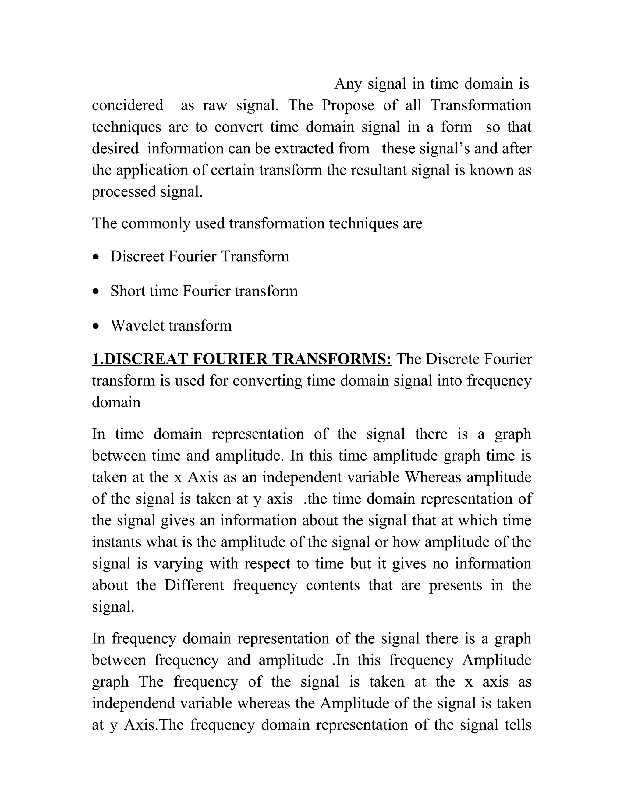
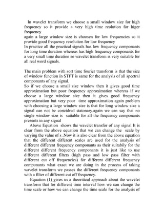
![2 SHOT TIME FOURIER TRANSFORM:
The Short time Fourier Transform is a modified version of Fourier
transform. S.T.F.T. is nothing it is simply the Fourier transform of
any signal multiplied by a window function.
STFTX
(w)
(t, f) = ∫t [x(t). w*( t – t')].e-j2Πf t
dt …….6.3
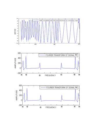
The basic idea behind the STFT is that any non stationary signal
can be considered stationary for a short time interval. So we can
say that the STFT gives an idea about time frequency and
amplitude
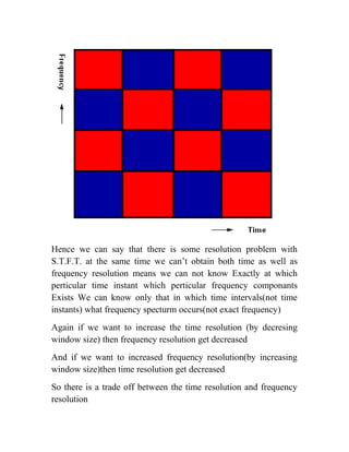
But again the problem with STFT is that how to choose the size of
window (time interval of window) because if we choose
A small size window than it will give good time resolution but
poor frequency resolution i.e. it gives good information about the
time but its frequency information is poor.
Again if we choose large size window than it will provide us a
very good frequency information but the time information is poor
again if we choose the large size of window then the signal can not
be considered stationary(because the signal is stationary only for
the short time interval)
Again at the same time we can’t get good time and frequency
resolution either we get good time resolution or good frequency
resolution
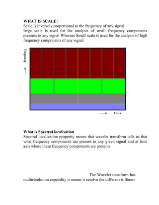
The small window size is suitable for high frequencies whereas
Large window size is suitable for low frequencies](https://image.slidesharecdn.com/bookwavelets-150723101626-lva1-app6892/85/Book-wavelets-10-320.jpg)
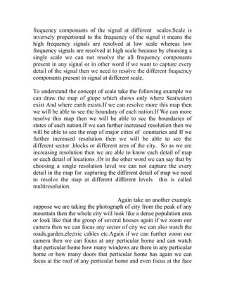
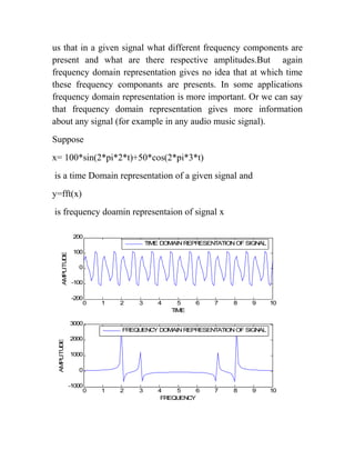
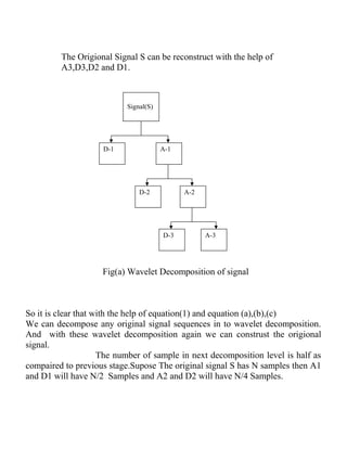
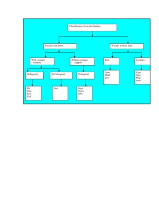
 cofficient of the signal
The output of High pass filter is called Detailed [D1](High freqency
componants) Cofficients Of the signal.
This Approximate cofficient[A1] again passed through a low pass and
high pass filter
And again Decompose the signal into Approximate[A 2] and Detailed
Cofficients[D 2]
Further Approximate Componants[A2] can be decomposed into
Approximate cofficients[A3] And Detailed Cofficients[D3]
The number of Decomposition levels depends on the length of signal and
our requirements
S =A1+D1 [First level Wavelet Decomposition]…(a)
A1=A2+D2 [Second level Wavelet Decomposition]…(b)
A2=A3+D3 [Third level Wavelet Decomposition]…(c)
S=A3+D3+D2+D1 ………………………………….(1)](https://image.slidesharecdn.com/bookwavelets-150723101626-lva1-app6892/85/Book-wavelets-19-320.jpg)
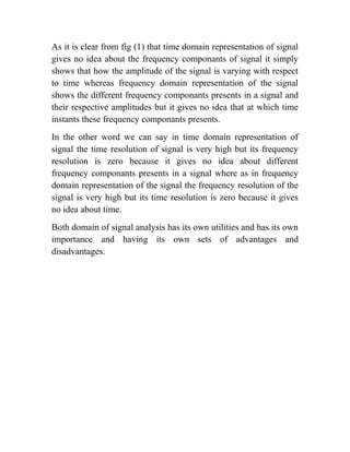
![So wavelet transform is highly suitable for the analysis of local
behaviour of the signal such as spikes or discontinuties. Because at
the point of discontinuty the frequencies changes very fast only for
a very littile time so by choosing suitable time scale we can also
study or analysis these sudden changes.
Again an another advantage of wavelet transform over fourier
transform is that the fourier transform convert the signal into the
different sinusoids of different different frequencies
The shape of sine and cosine waves are predefined and
predectable.wheareas in wavelet transform we convert the signal
into the mother wavelets of different amplitude and scale the local
behavour of any signal can be discribed in better way by using
wavelets
Again with W.T. we have a freedom to choose the shape of
wavelets (mother wavelet).there are lot of standard wavelets
families (wavelet families contain different wavelets of different
orders) suitable for different applications.
Again with wavelet transform we have freedom to design our own
wavelet hence we can define our own wavelet by defining Two
functions
[1]Wavelet function:
[2]Scale function:
[1] Wavelet function: wavelet function capture the details(high
frequencies) present in any signal And the intrgation of wavelet
function should be zero or the mean value of wavelet function
should be zero
∫ Ψ(x).d(x)=0
[2] Scale function: Scale function capture the low frequencies
information(approximate ) presents in any signal.the intregation of
scale function should be one it means its average value is one.
∫Ǿ(x).d(x)=1](https://image.slidesharecdn.com/bookwavelets-150723101626-lva1-app6892/85/Book-wavelets-21-320.jpg)
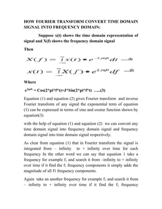
![[1]the support of wavelet function Ψ(t) and scaling function Ǿ(x):-
This is the most important criteria that the wavelet function and
scaling function have compact support or not have compact
support.This properity of wavelet decides the localisation of
wavelet in time and frequency domain.the support of wavelet
function decides
the speed of convergence to 0 of wavelet function (Ψ(t) or Ψ(w))
when the time t or the frequency w goes to infinity.
[2] wavelet with F.I.R. filter or without F.I.R. filter:
[3] Symmetry of wavelets: wavelet is symmetric,near symmetric or
asymetric
[4] Orthogonality or biorthogonality
[5] Regularity of wavelet wich decide the smoothness of
reconstructing signal or image is a very important criteria.
[6] the number of vanishing moment (zero moment)for wavelet
function Ψ or scaling function Ǿ this is very useful for
compression purpose.
[7] the scaling function exist or does not exist
[8] an explict mathamatical expression available or not for scaling
function (if exist) and wavelet function
[9]Continue or discreate](https://image.slidesharecdn.com/bookwavelets-150723101626-lva1-app6892/85/Book-wavelets-24-320.jpg)
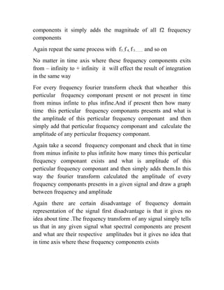
The document discusses various signal transformation techniques, primarily focusing on the Fourier Transform (FT), Short Time Fourier Transform (STFT), and Wavelet Transform (WT) for analyzing signals in time and frequency domains. FT provides frequency information but lacks time resolution, while STFT offers a time-frequency analysis with a trade-off in resolution depending on window size. WT enhances this by using different window sizes for different frequency components, thus allowing better time localization for high frequencies and is deemed more suitable for real-world signals.


![[Deck] What's New in Spark-Iceberg Integration via DSV2.pptx](https://cdn.slidesharecdn.com/ss_thumbnails/deckwhatsnewinspark-icebergintegrationviadsv2-260210005337-25955b12-thumbnail.jpg?width=640&height=640&fit=bounds)


