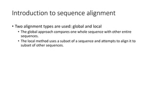
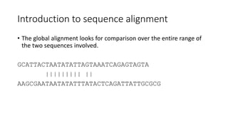
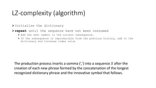


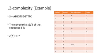
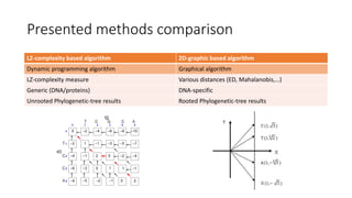
![LZ-complexity based sequence comparison
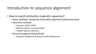
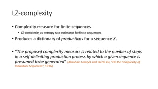
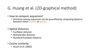
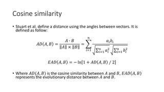
• The sequence similarity matrix 𝑀 is built using the following
formulas:
𝑀 𝑖, 0 = 𝑘=1
𝑖
𝜎 𝑆𝑖, _
𝑀 0, 𝑗 = 𝑘=1
𝑗
𝜎 _, 𝑄𝑗
𝑀[𝑖, 𝑗] = min
𝑀 𝑖 − 1, 𝑗 + 𝜎(𝑆𝑖, _)
𝑀 𝑖 − 1, 𝑗 − 1 + 𝜎(𝑆𝑖, 𝑄𝑖)
𝑀 𝑖, 𝑗 − 1 + 𝜎(_, 𝑄𝑖)
𝑀 𝑖 − 1, 𝑗 − 1 𝑀 𝑖 − 1, 𝑗
𝑀 𝑖, 𝑗 − 1](https://image.slidesharecdn.com/presentazione-150912084416-lva1-app6892/85/Biological-sequences-analysis-29-320.jpg)
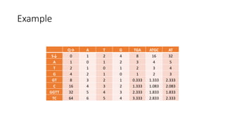
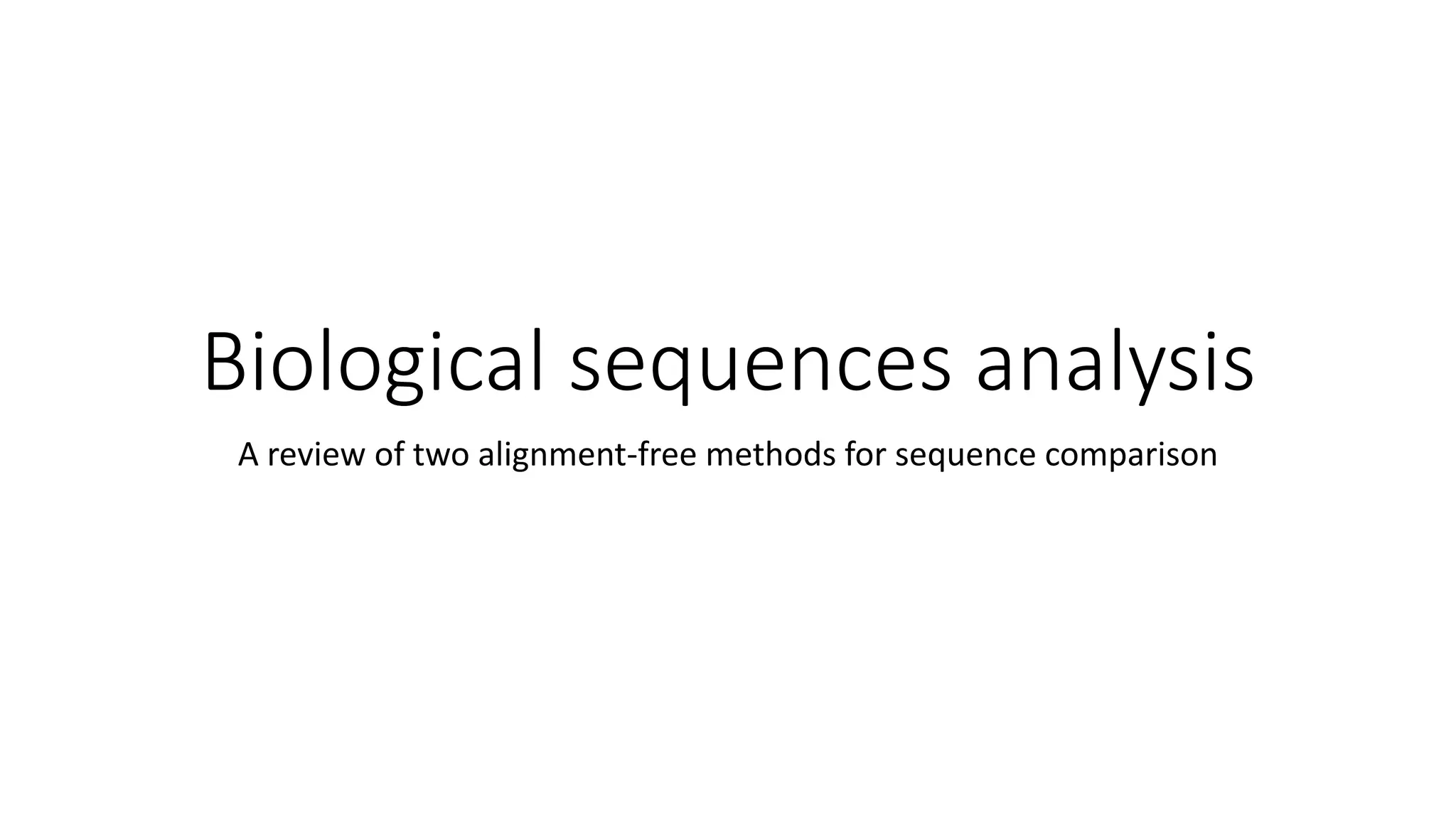
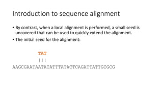
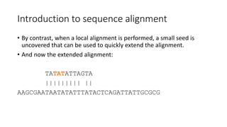
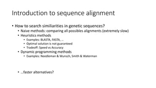
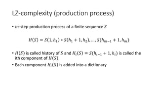
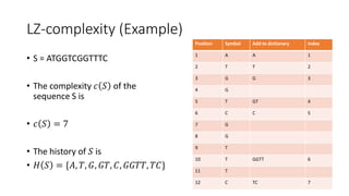
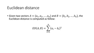
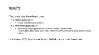
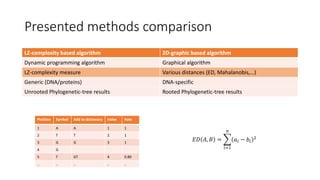
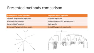
![Example
𝑀[𝑚, 𝑛] is the similarity distance between sequences 𝑆 and 𝑄
Q→ A T G TGA ATGC AT
S↓ 0 1 2 4 8 16 32
A 1 0 1 2 3 4 5
T 2 1 0 1 2 3 4
G 4 2 1 0 1 2 3
GT 8 3 2 1 0.333 1.333 2.333
C 16 4 3 2 1.333 1.083 2.083
GGTT 32 5 4 3 2.333 1.833 1.833
TC 64 6 5 4 3.333 2.833 2.333](https://image.slidesharecdn.com/presentazione-150912084416-lva1-app6892/85/Biological-sequences-analysis-31-320.jpg)
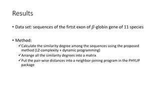
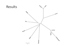
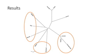
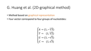
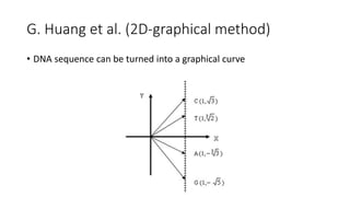
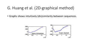
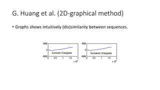
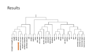
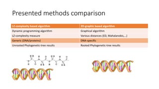


The document reviews two alignment-free methods for biological sequence comparison: an LZ-complexity based method and a 2D graphical method. It highlights the inefficiencies of traditional alignment-based algorithms and presents the advantages of alignment-free approaches, which typically operate in linear time. Additionally, it discusses various distance metrics for sequence comparison, including Euclidean and Mahalanobis distances, demonstrating their applications in analyzing genetic sequences.


![Polymer [ बहुलक ] Chemistry Notes PDF - Irfanullah Mehar - JJ Sir Chemistry.pdf](https://cdn.slidesharecdn.com/ss_thumbnails/polymerchemistrynotespdf-irfanullahmehar-jjsirchemistry-260210172118-3f9b37f7-thumbnail.jpg?width=640&height=640&fit=bounds)


