Logistic regression 3

1. Logistic Regression
Jeff Witmer
30 March 2016

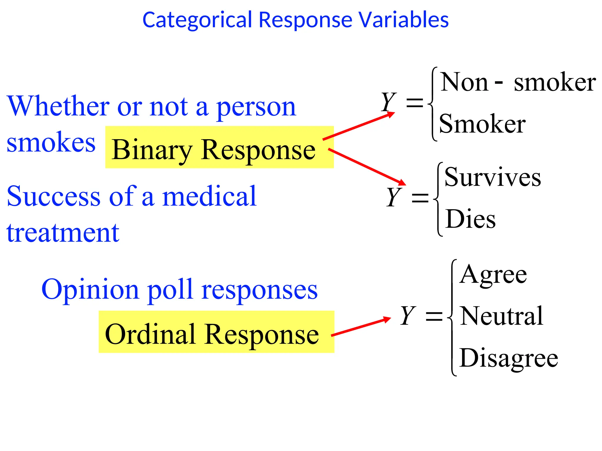
2. Categorical Response Variables
Examples:
Whether or not a person
smokes 

 

Smoker
smoker
Non
Y
Success of a medical
treatment 



Dies
Survives
Y
Opinion poll responses






Disagree
Neutral
Agree
Y
Binary Response
Ordinal Response

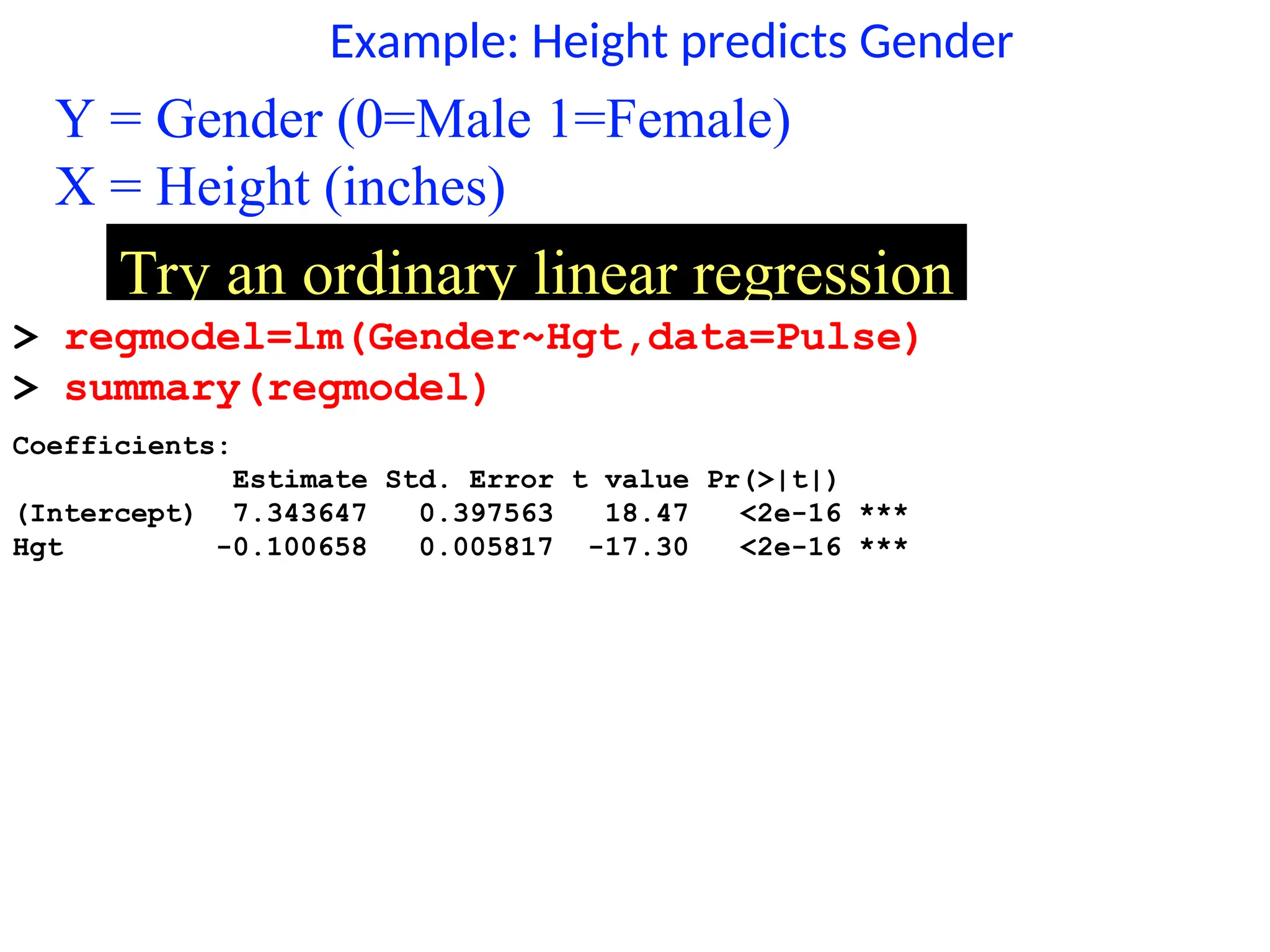
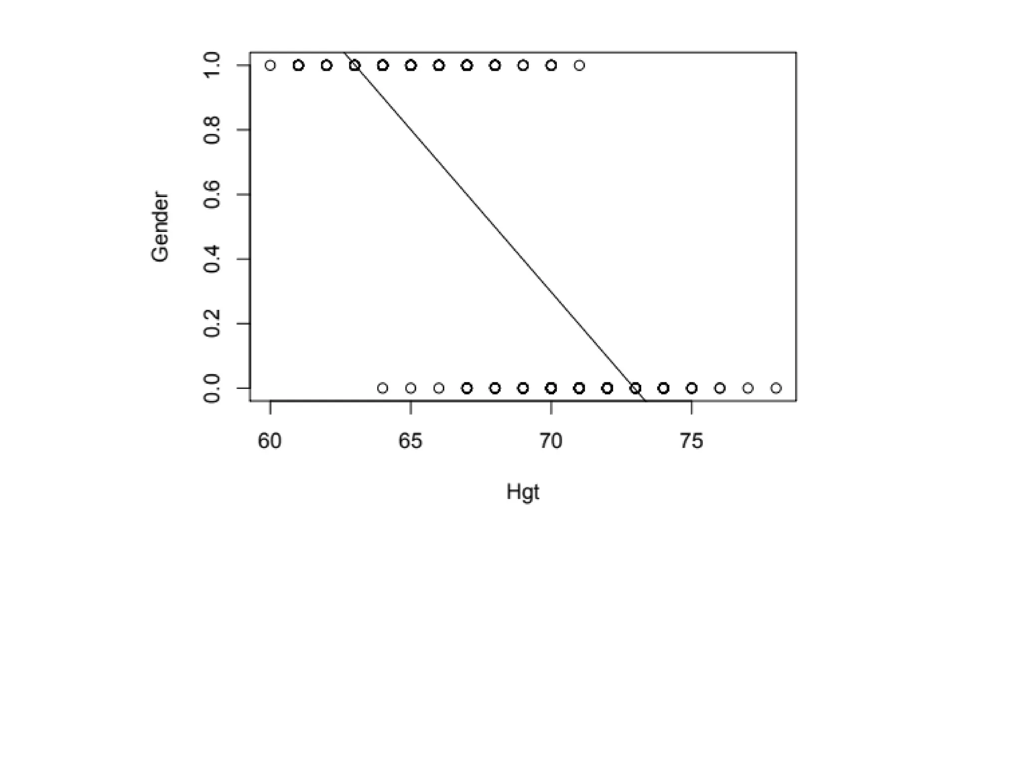
3. Example: Height predicts Gender
Y = Gender (0=Male 1=Female)
X = Height (inches)
Try an ordinary linear regression
> regmodel=lm(Gender~Hgt,data=Pulse)
> summary(regmodel)
Coefficients:
Estimate Std. Error t value Pr(>|t|)
(Intercept) 7.343647 0.397563 18.47 <2e-16 ***
Hgt -0.100658 0.005817 -17.30 <2e-16 ***

5. Ordinary linear regression is used a lot, and is
taught in every intro stat class. Logistic regression
is rarely taught or even mentioned in intro stats,
but mostly because of inertia.
We now have the computing power and
software to implement logistic regression.

6. π = Proportion of “Success”
In ordinary regression the model predicts the
mean Y for any combination of predictors.
What’s the “mean” of a 0/1 indicator variable?
success"
"
of
Proportion
trials
of
#
'
1
of
#




s
n
y
y i
Goal of logistic regression: Predict the “true”
proportion of success, π, at any value of the
predictor.

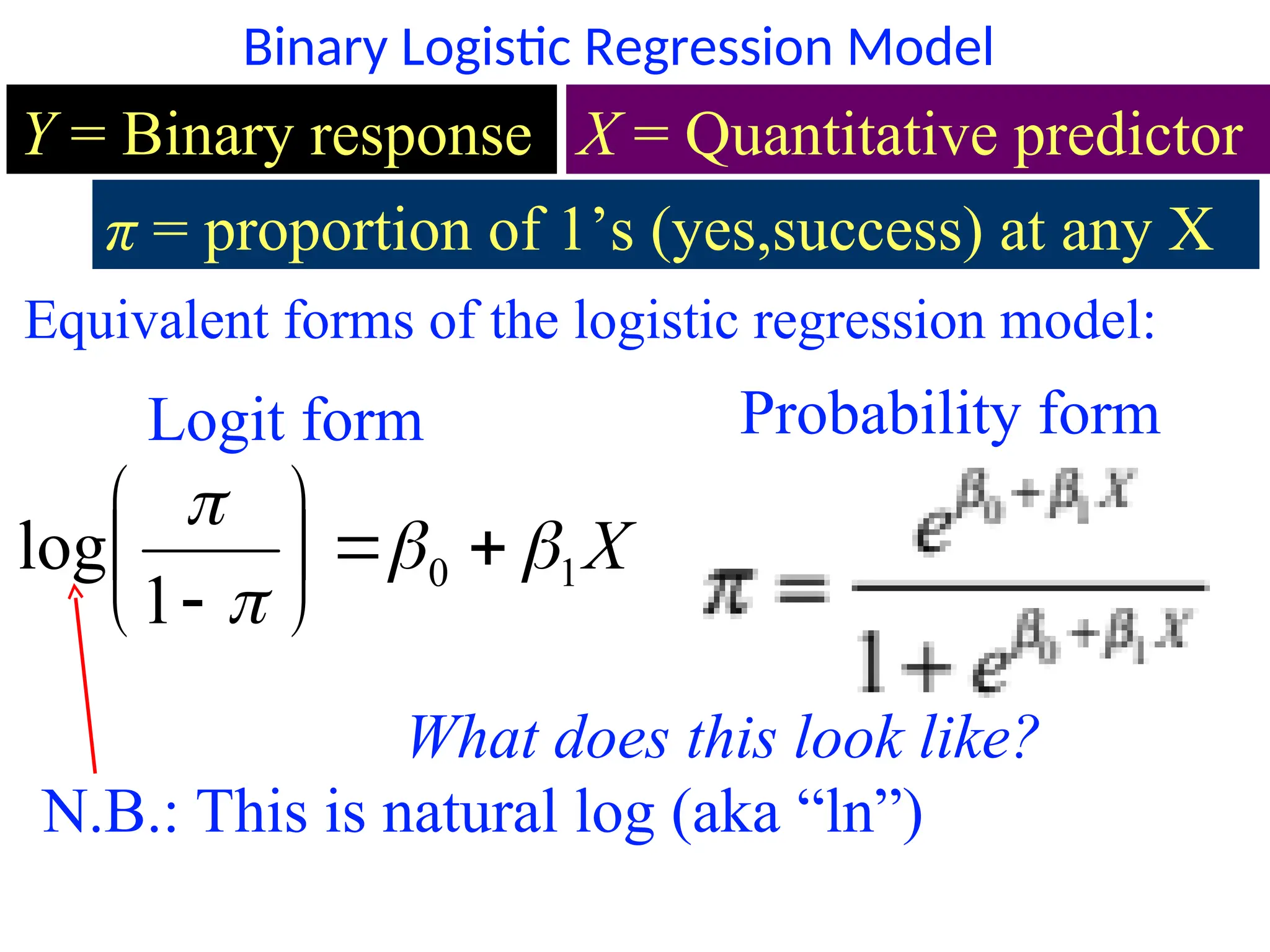
7. Binary Logistic Regression Model
Y = Binary response X = Quantitative predictor
π = proportion of 1’s (yes,success) at any X
Equivalent forms of the logistic regression model:
What does this look like?
X
1
0
1
log 












Logit form Probability form
N.B.: This is natural log (aka “ln”)

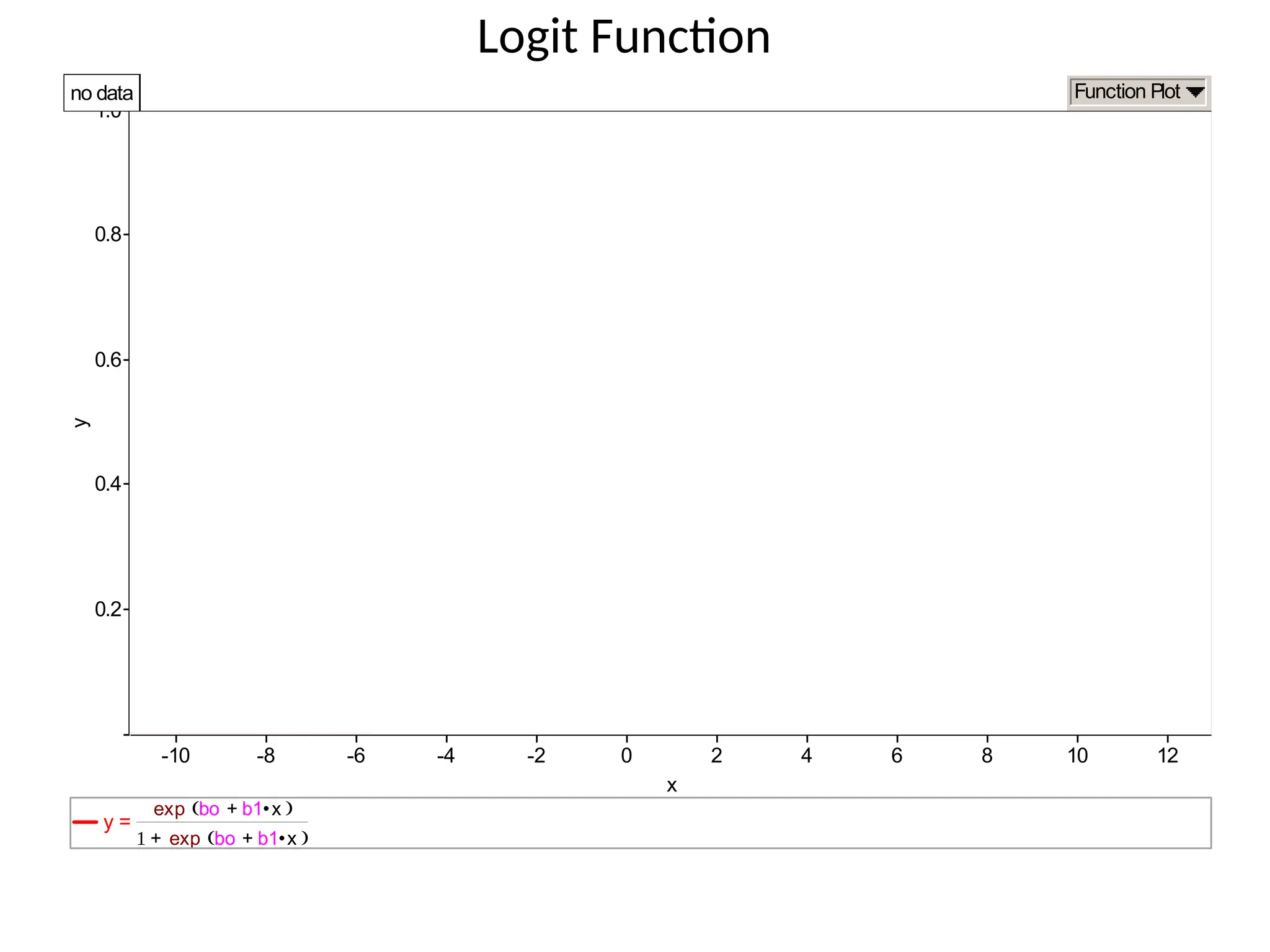
8. y
0.2
0.4
0.6
0.8
1.0
x
-10 -8 -6 -4 -2 0 2 4 6 8 10 12
y =
bo b1 x
•
+
 
exp
 bo b1 x
•
+
 
exp
+
no data Function Plot
Logit Function

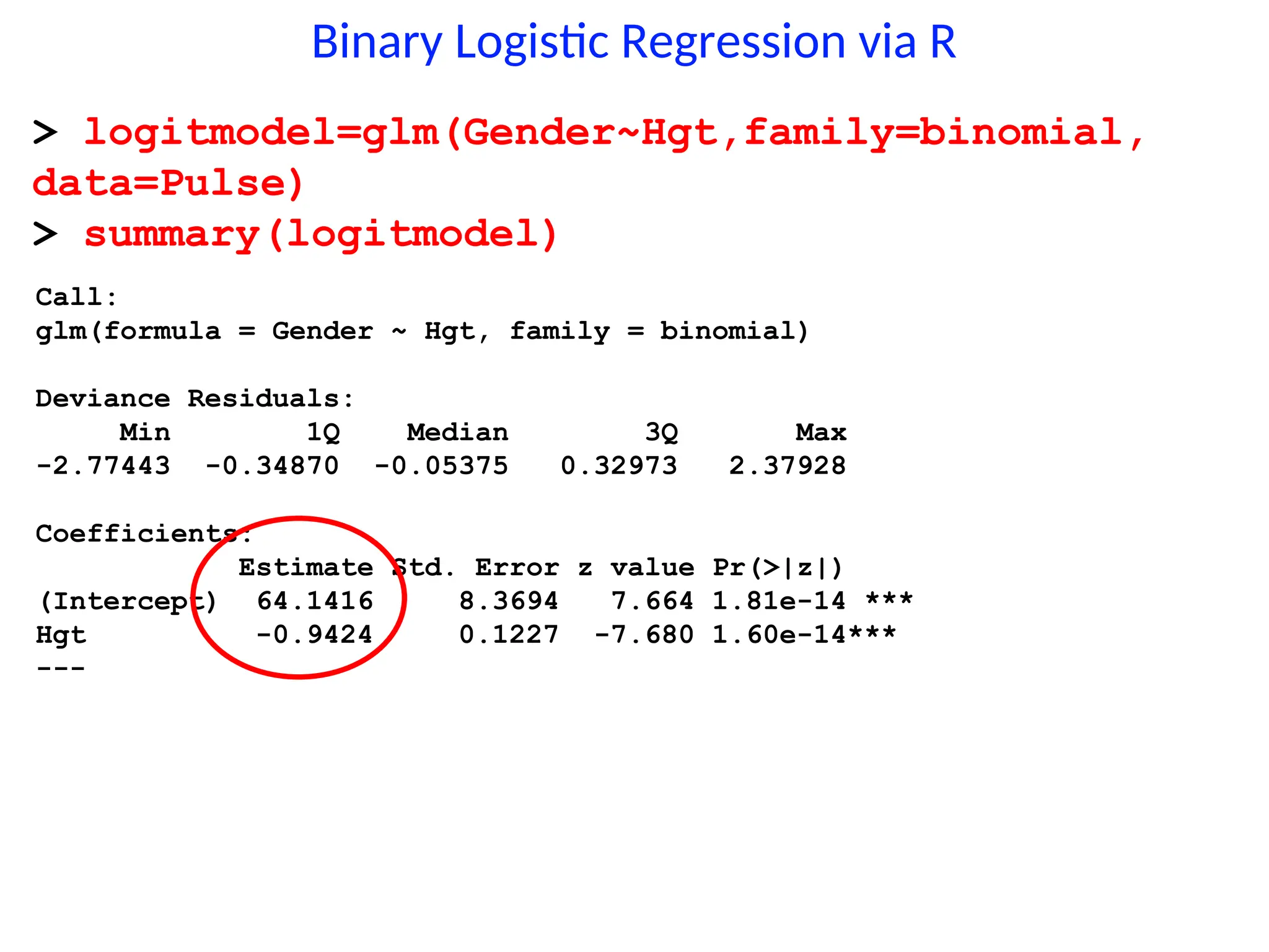
9. Binary Logistic Regression via R
> logitmodel=glm(Gender~Hgt,family=binomial,
data=Pulse)
> summary(logitmodel)
Call:
glm(formula = Gender ~ Hgt, family = binomial)
Deviance Residuals:
Min 1Q Median 3Q Max
-2.77443 -0.34870 -0.05375 0.32973 2.37928
Coefficients:
Estimate Std. Error z value Pr(>|z|)
(Intercept) 64.1416 8.3694 7.664 1.81e-14 ***
Hgt -0.9424 0.1227 -7.680 1.60e-14***
---

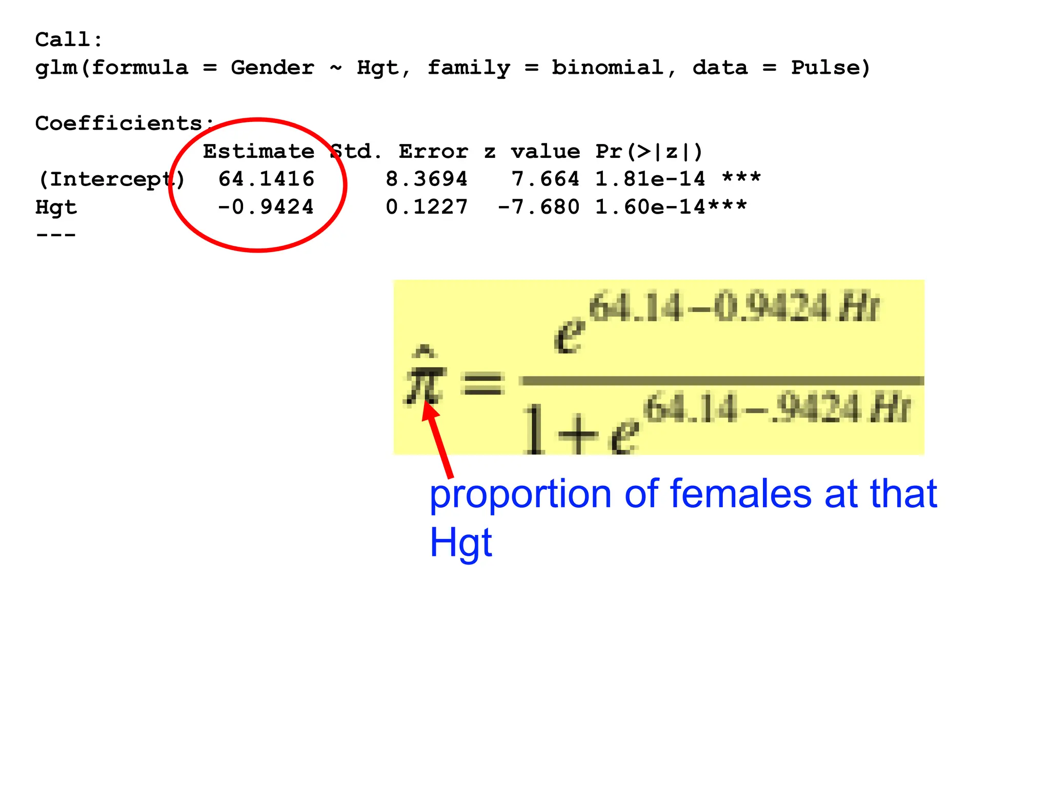
10. proportion of females at that
Hgt
Call:
glm(formula = Gender ~ Hgt, family = binomial, data = Pulse)
Coefficients:
Estimate Std. Error z value Pr(>|z|)
(Intercept) 64.1416 8.3694 7.664 1.81e-14 ***
Hgt -0.9424 0.1227 -7.680 1.60e-14***
---

11. > plot(fitted(logitmodel)~Pulse$Hgt)

12. > with(Pulse,plot(Hgt,jitter(Gender,amount=0.05)))
> curve(exp(64.1-0.94*x)/(1+exp(64.1-0.94*x)), add=TRUE)

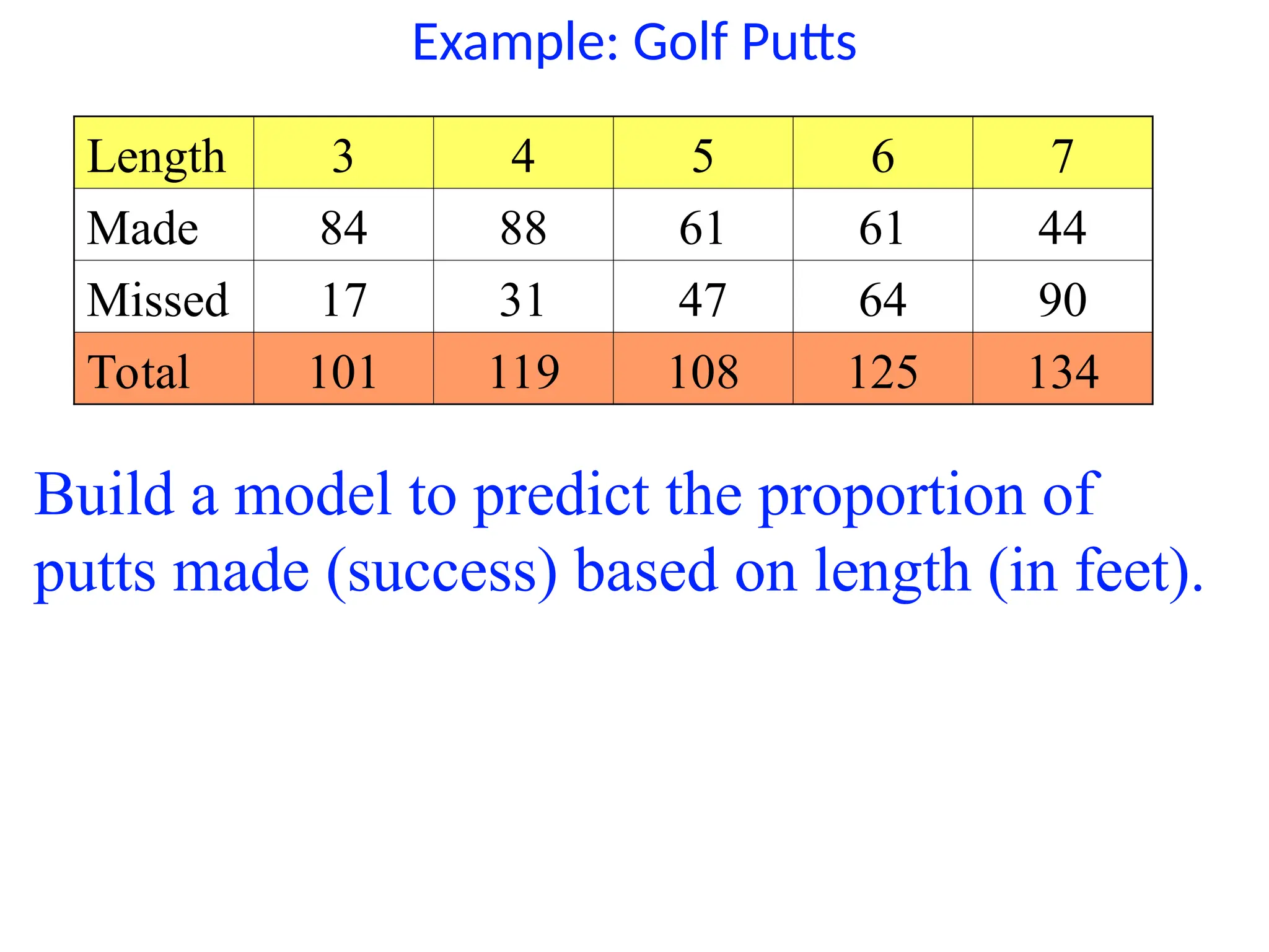
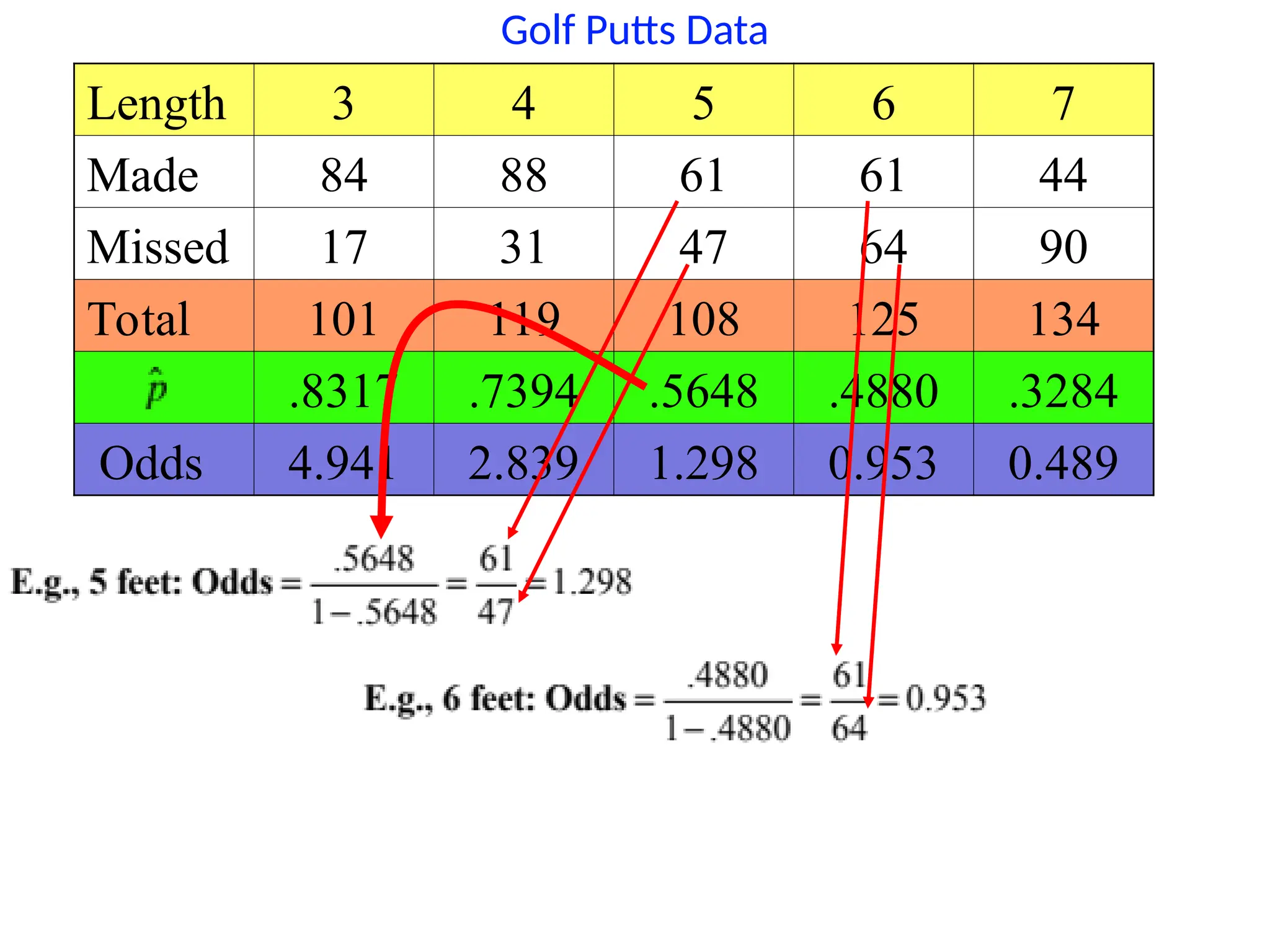
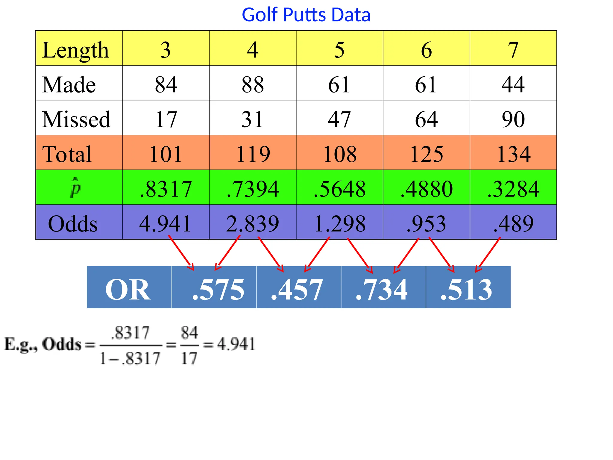
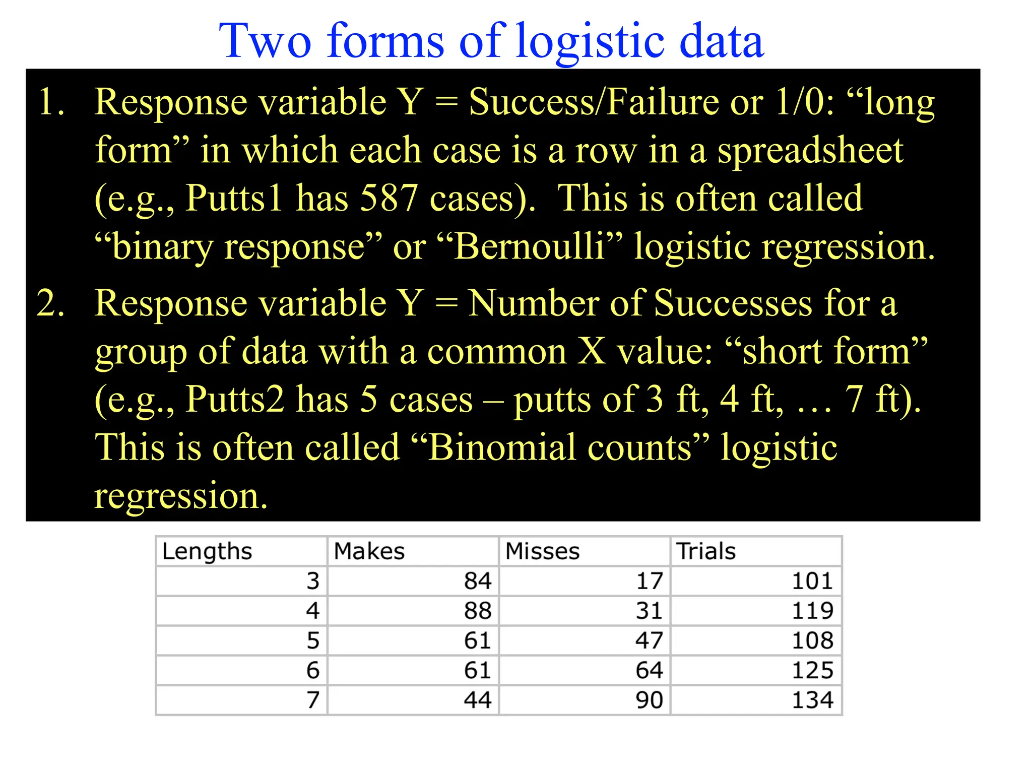
13. Example: Golf Putts
Length 3 4 5 6 7
Made 84 88 61 61 44
Missed 17 31 47 64 90
Total 101 119 108 125 134
Build a model to predict the proportion of
putts made (success) based on length (in feet).

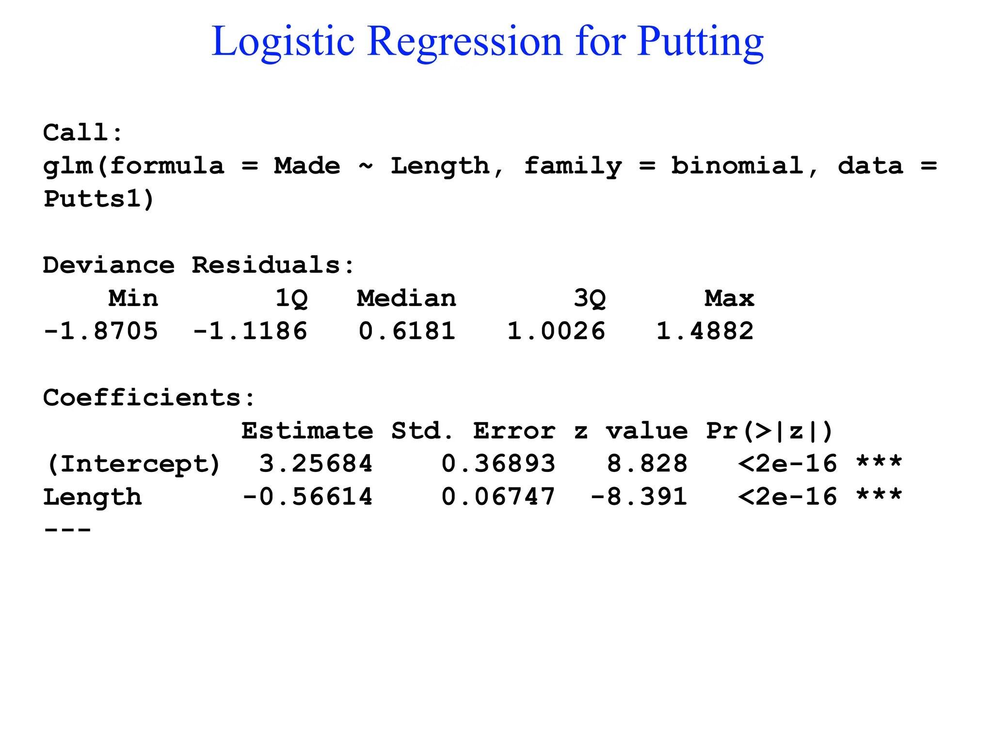
14. Logistic Regression for Putting
Call:
glm(formula = Made ~ Length, family = binomial, data =
Putts1)
Deviance Residuals:
Min 1Q Median 3Q Max
-1.8705 -1.1186 0.6181 1.0026 1.4882
Coefficients:
Estimate Std. Error z value Pr(>|z|)
(Intercept) 3.25684 0.36893 8.828 <2e-16 ***
Length -0.56614 0.06747 -8.391 <2e-16 ***
---

15. 3 4 5 6 7
-0.5
0.0
0.5
1.0
1.5
PuttLength
logitPropMade
Linear part of
logistic fit

16. Probability Form of Putting Model
2 4 6 8 10 12
0.0
0.2
0.4
0.6
0.8
1.0
PuttLength
Probability
Made Length
Length
e
e
566
.
0
257
.
3
566
.
0
257
.
3
1
ˆ 





17. Odds
Definition:



1 )
(
)
(
No
P
Yes
P
 is the odds of Yes.
odds
odds
odds





1
1




18. Fair die
Prob Odds
Event
roll a 2 1/6 1/5 [or 1/5:1 or 1:5]
even # 1/2 1 [or 1:1]
X > 2 2/3 2 [or 2:1]

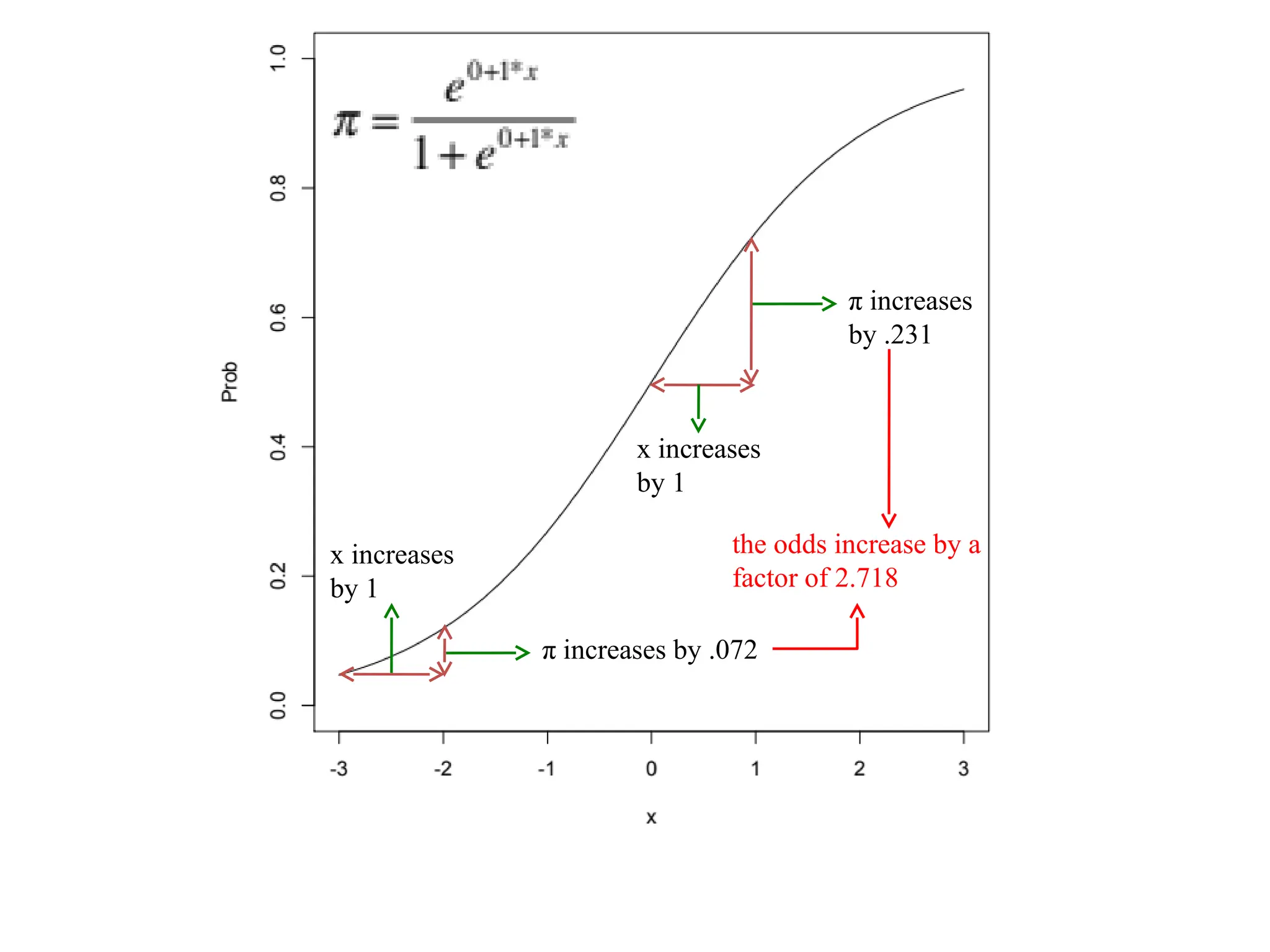
19. x increases
by 1
x increases
by 1
π increases by .072
π increases
by .231
the odds increase by a
factor of 2.718

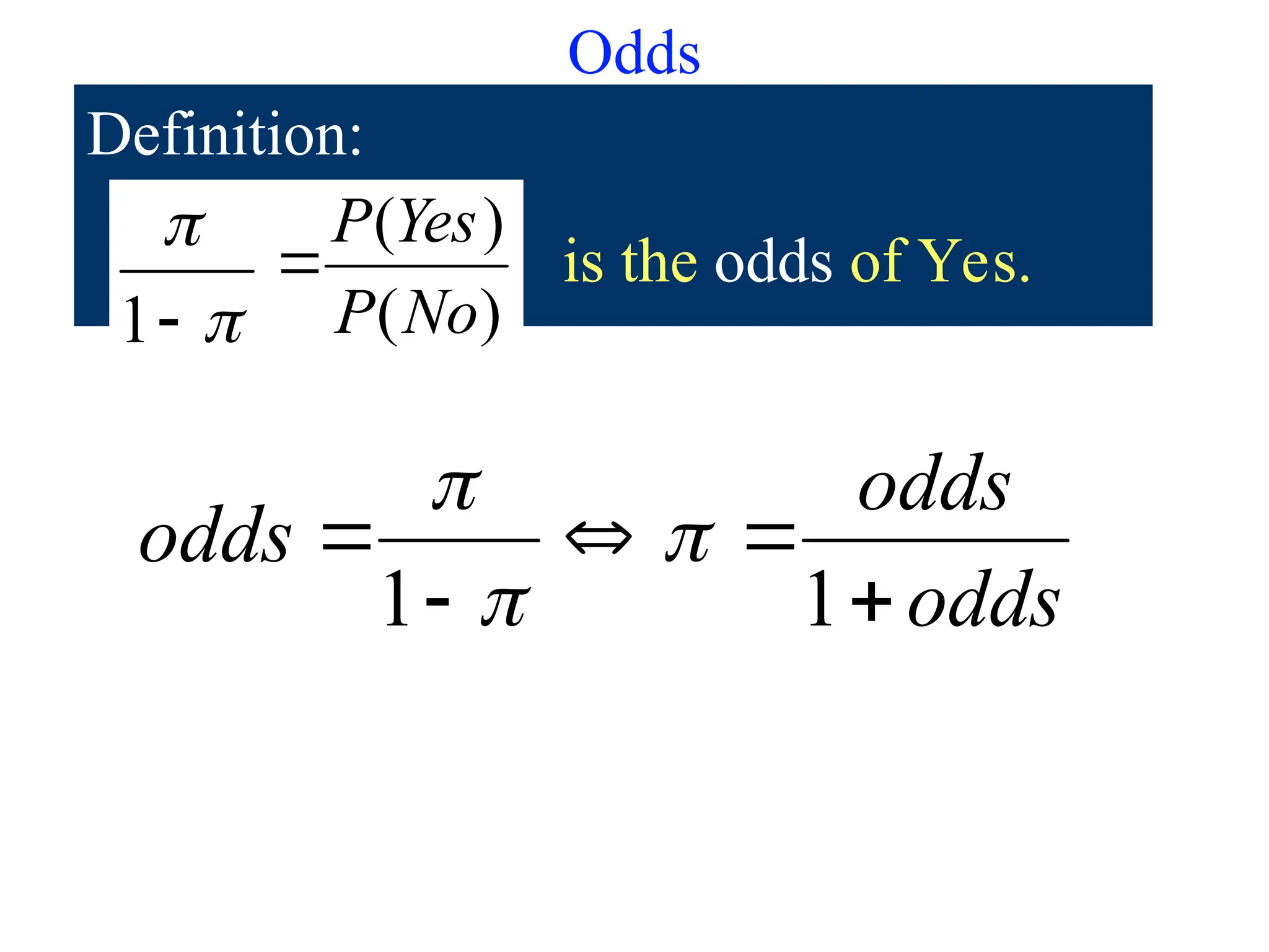
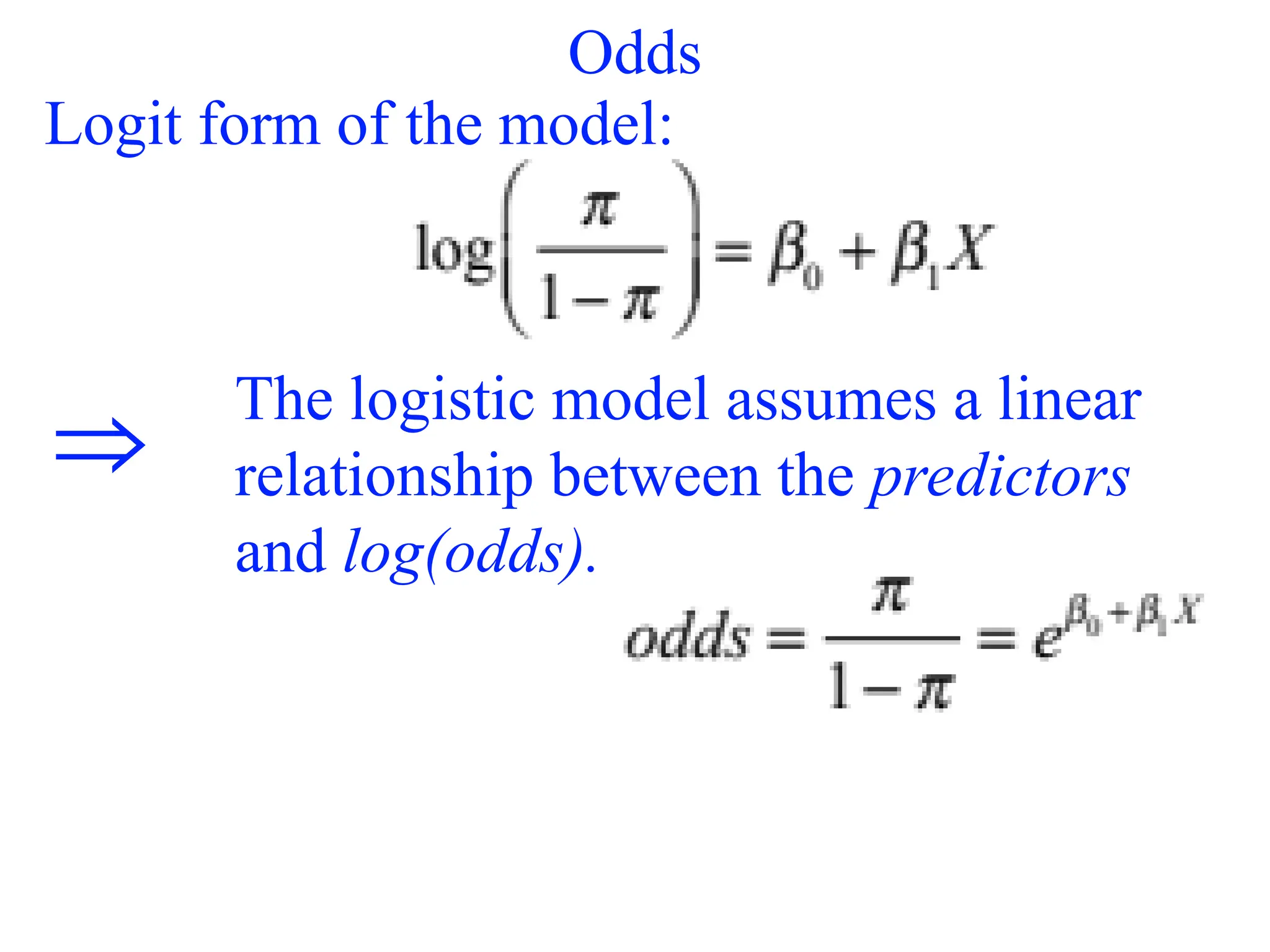
20. Odds
The logistic model assumes a linear
relationship between the predictors
and log(odds).
⇒
Logit form of the model:

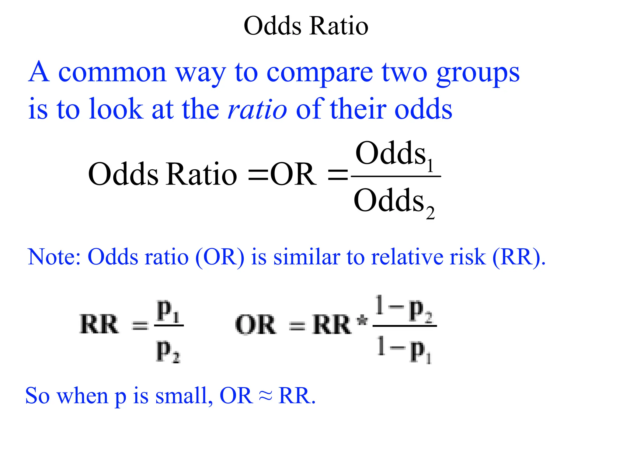
21. Odds Ratio
A common way to compare two groups
is to look at the ratio of their odds
2
1
Odds
Odds
OR
Ratio
Odds 

Note: Odds ratio (OR) is similar to relative risk (RR).
So when p is small, OR ≈ RR.

22. X is replaced by X + 1:
is replaced by
So the ratio is

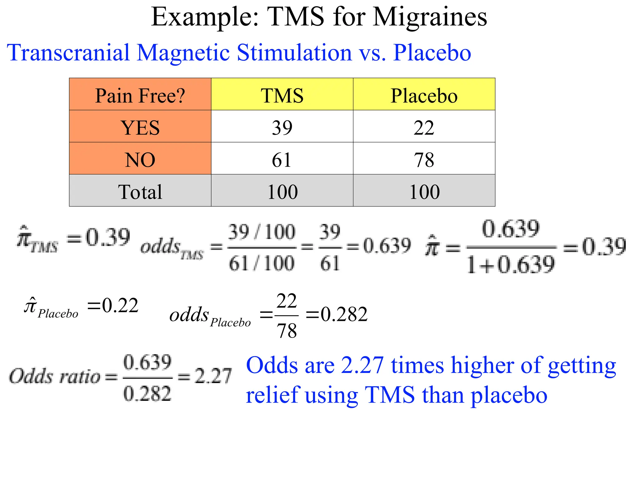
23. Example: TMS for Migraines
Transcranial Magnetic Stimulation vs. Placebo
Pain Free? TMS Placebo
YES 39 22
NO 61 78
Total 100 100
22
.
0
ˆ 
Placebo
 282
.
0
78
22


Placebo
odds
Odds are 2.27 times higher of getting
relief using TMS than placebo

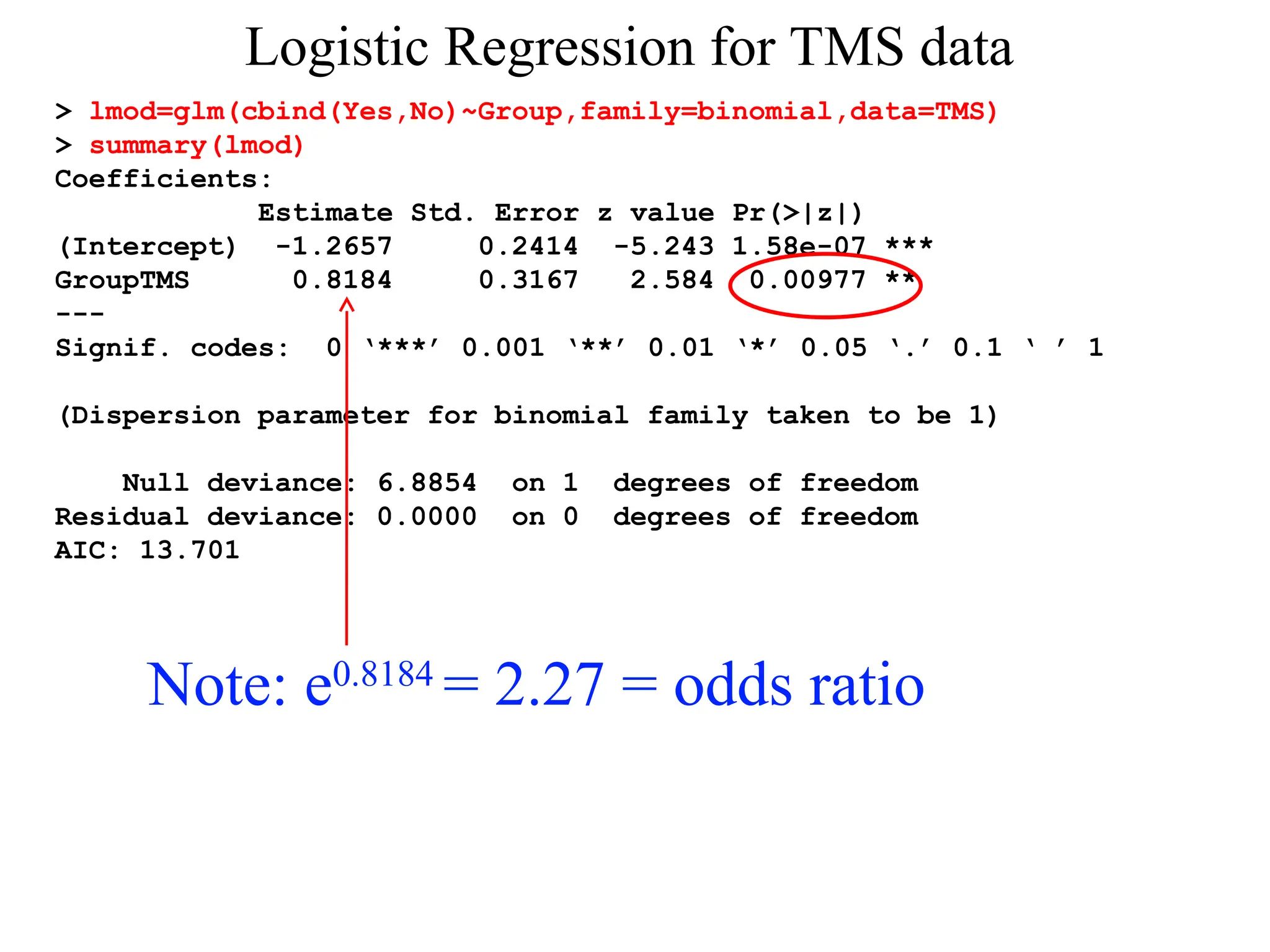
24. Logistic Regression for TMS data
> lmod=glm(cbind(Yes,No)~Group,family=binomial,data=TMS)
> summary(lmod)
Coefficients:
Estimate Std. Error z value Pr(>|z|)
(Intercept) -1.2657 0.2414 -5.243 1.58e-07 ***
GroupTMS 0.8184 0.3167 2.584 0.00977 **
---
Signif. codes: 0 ‘***’ 0.001 ‘**’ 0.01 ‘*’ 0.05 ‘.’ 0.1 ‘ ’ 1
(Dispersion parameter for binomial family taken to be 1)
Null deviance: 6.8854 on 1 degrees of freedom
Residual deviance: 0.0000 on 0 degrees of freedom
AIC: 13.701
Note: e0.8184
= 2.27 = odds ratio

25. > datatable=rbind(c(39,22),c(61,78))
> datatable
[,1] [,2]
[1,] 39 22
[2,] 61 78
> chisq.test(datatable,correct=FALSE)
Pearson's Chi-squared test
data: datatable
X-squared = 6.8168, df = 1, p-value = 0.00903
> lmod=glm(cbind(Yes,No)~Group,family=binomial,data=TMS)
> summary(lmod)
Call:
glm(formula = cbind(Yes, No) ~ Group, family = binomial)Coefficients:
Estimate Std. Error z value Pr(>|z|)
(Intercept) -1.2657 0.2414 -5.243 1.58e-07 ***
GroupTMS 0.8184 0.3167 2.584 0.00977 **
Binary Logistic Regression
Chi-Square Test for
2-way table

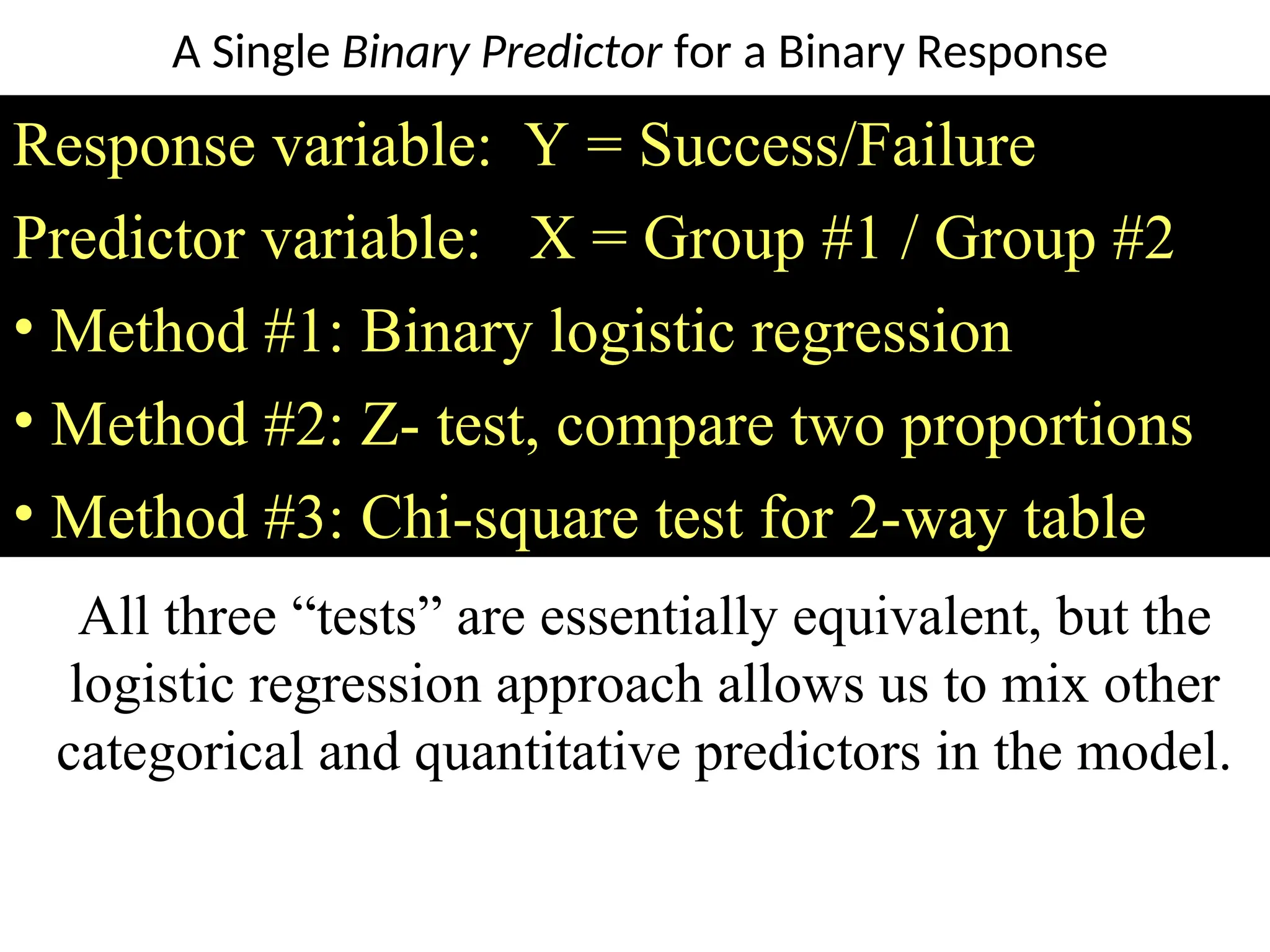
26. Response variable: Y = Success/Failure
Predictor variable: X = Group #1 / Group #2
• Method #1: Binary logistic regression
• Method #2: Z- test, compare two proportions
• Method #3: Chi-square test for 2-way table
All three “tests” are essentially equivalent, but the
logistic regression approach allows us to mix other
categorical and quantitative predictors in the model.
A Single Binary Predictor for a Binary Response

27. Putting Data
Odds using data from 6 feet = 0.953
Odds using data from 5 feet = 1.298
 Odds ratio (6 ft to 5 ft) = 0.953/1.298 = 0.73
The odds of making a putt from 6 feet are
73% of the odds of making from 5 feet.

28. Golf Putts Data
Length 3 4 5 6 7
Made 84 88 61 61 44
Missed 17 31 47 64 90
Total 101 119 108 125 134
.8317 .7394 .5648 .4880 .3284
Odds 4.941 2.839 1.298 0.953 0.489

29. Golf Putts Data
Length 3 4 5 6 7
Made 84 88 61 61 44
Missed 17 31 47 64 90
Total 101 119 108 125 134
.8317 .7394 .5648 .4880 .3284
Odds 4.941 2.839 1.298 .953 .489
OR .575 .457 .734 .513

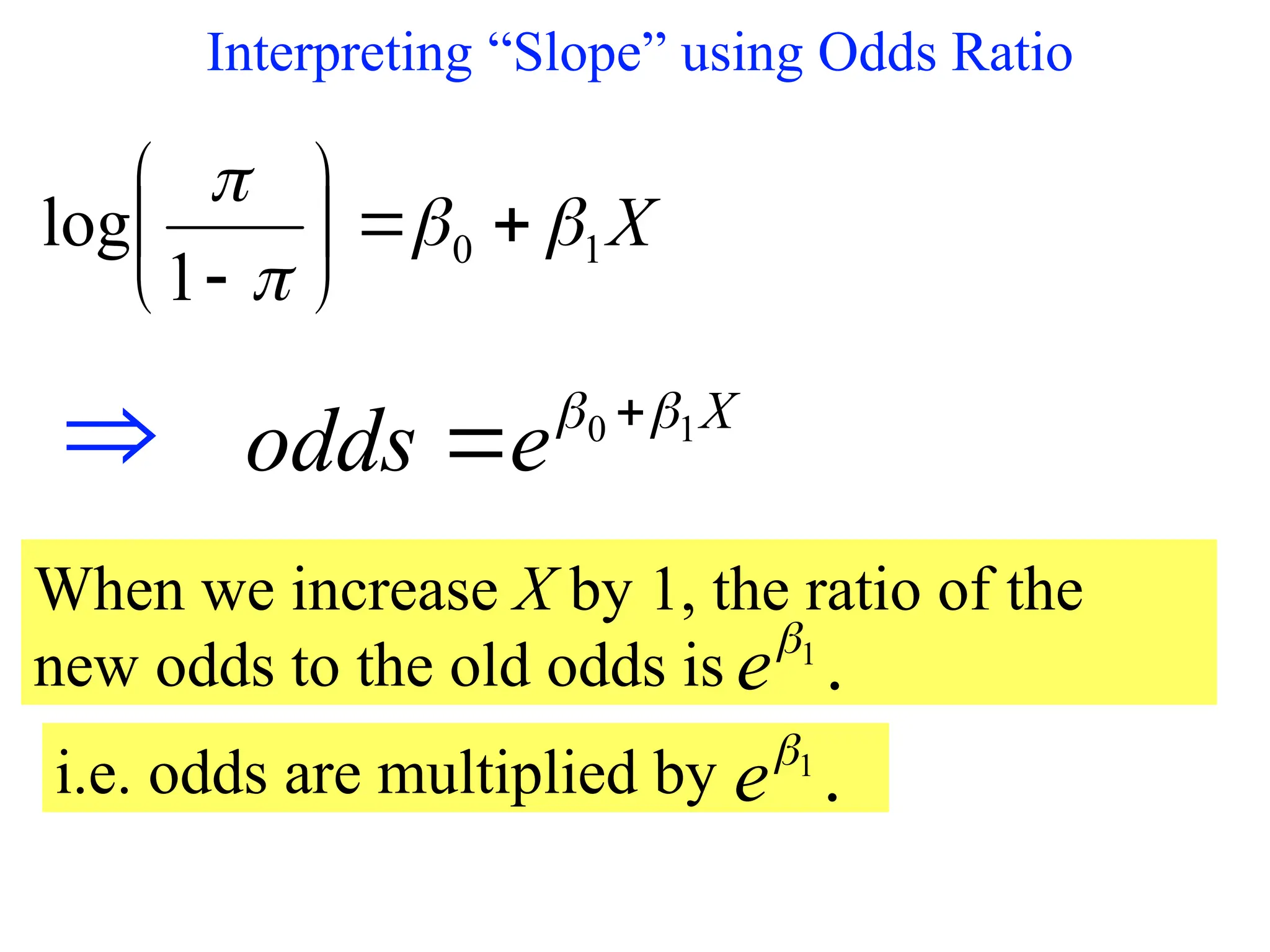
30. Interpreting “Slope” using Odds Ratio
X
1
0
1
log 












When we increase X by 1, the ratio of the
new odds to the old odds is .
1

e
X
e
odds 1
0 
 

⇒
i.e. odds are multiplied by .
1

e

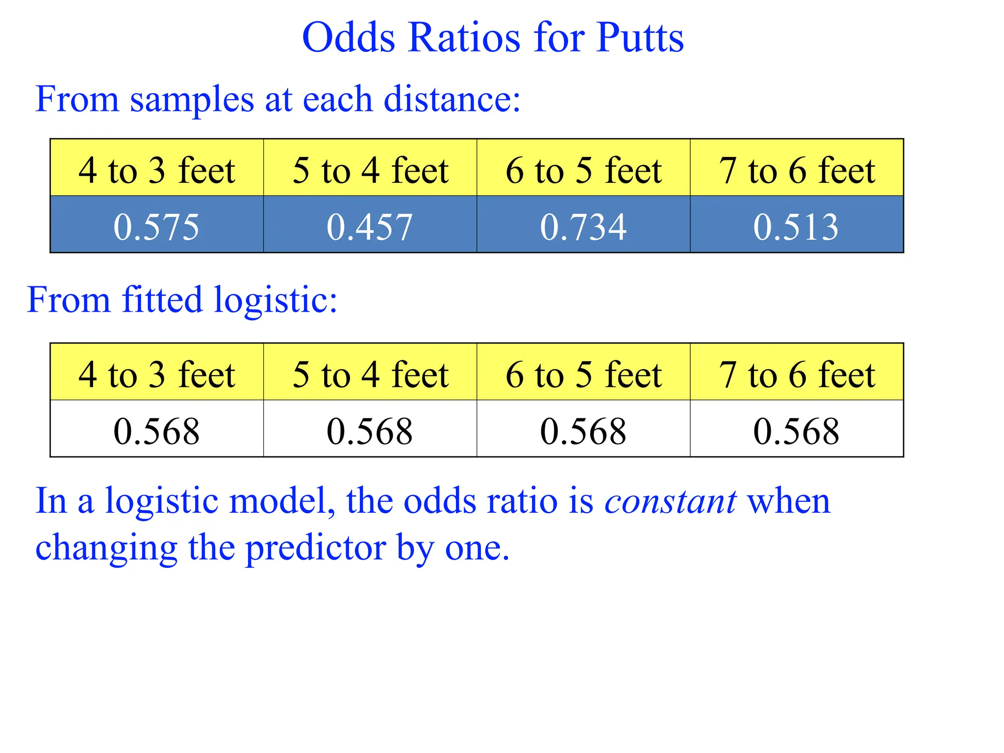
31. Odds Ratios for Putts
4 to 3 feet 5 to 4 feet 6 to 5 feet 7 to 6 feet
0.575 0.457 0.734 0.513
From samples at each distance:
4 to 3 feet 5 to 4 feet 6 to 5 feet 7 to 6 feet
0.568 0.568 0.568 0.568
From fitted logistic:
In a logistic model, the odds ratio is constant when
changing the predictor by one.

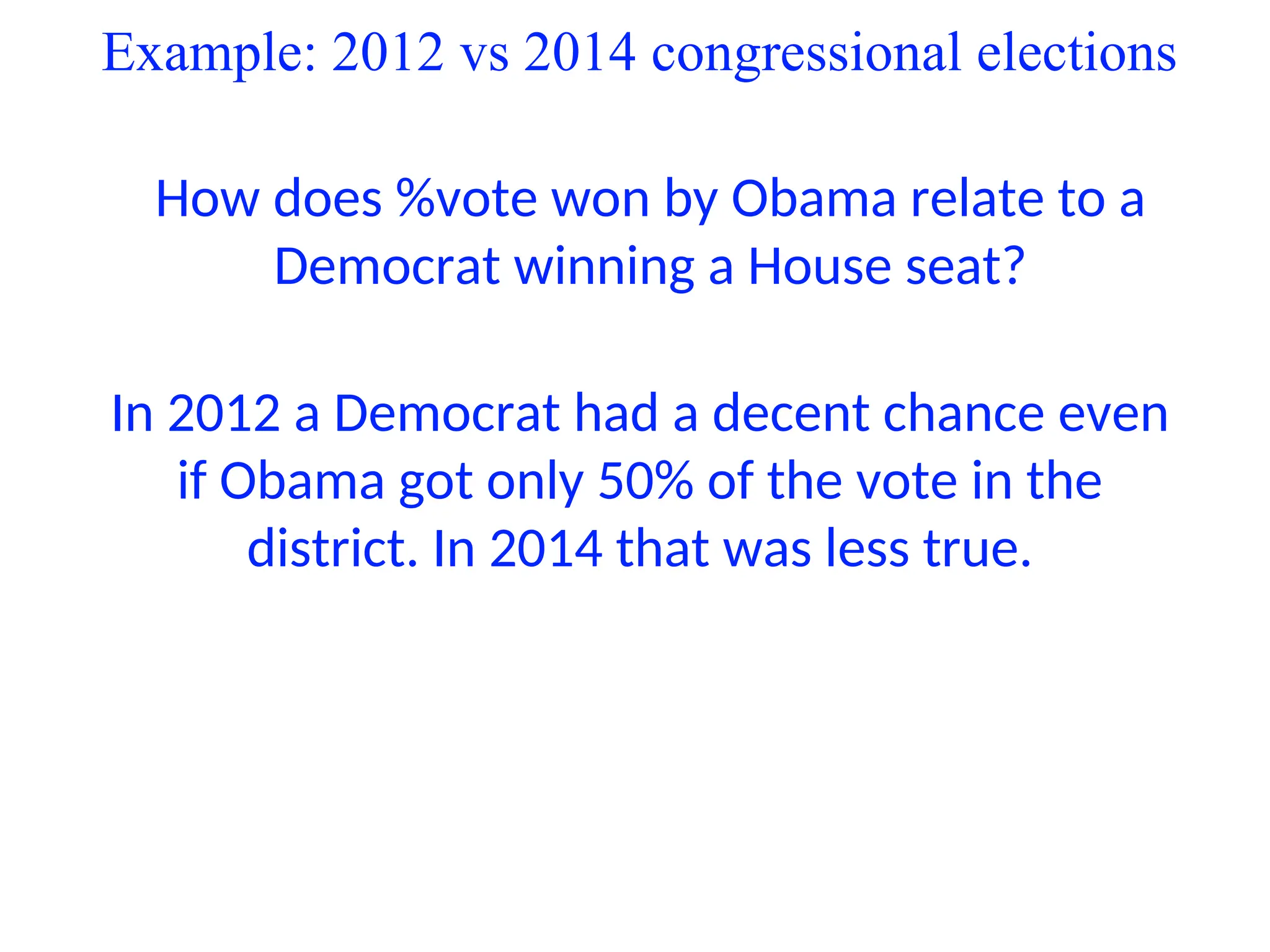
32. Example: 2012 vs 2014 congressional elections
How does %vote won by Obama relate to a
Democrat winning a House seat?
See the script elections 12, 14.R

33. Example: 2012 vs 2014 congressional elections
How does %vote won by Obama relate to a
Democrat winning a House seat?
In 2012 a Democrat had a decent chance even
if Obama got only 50% of the vote in the
district. In 2014 that was less true.

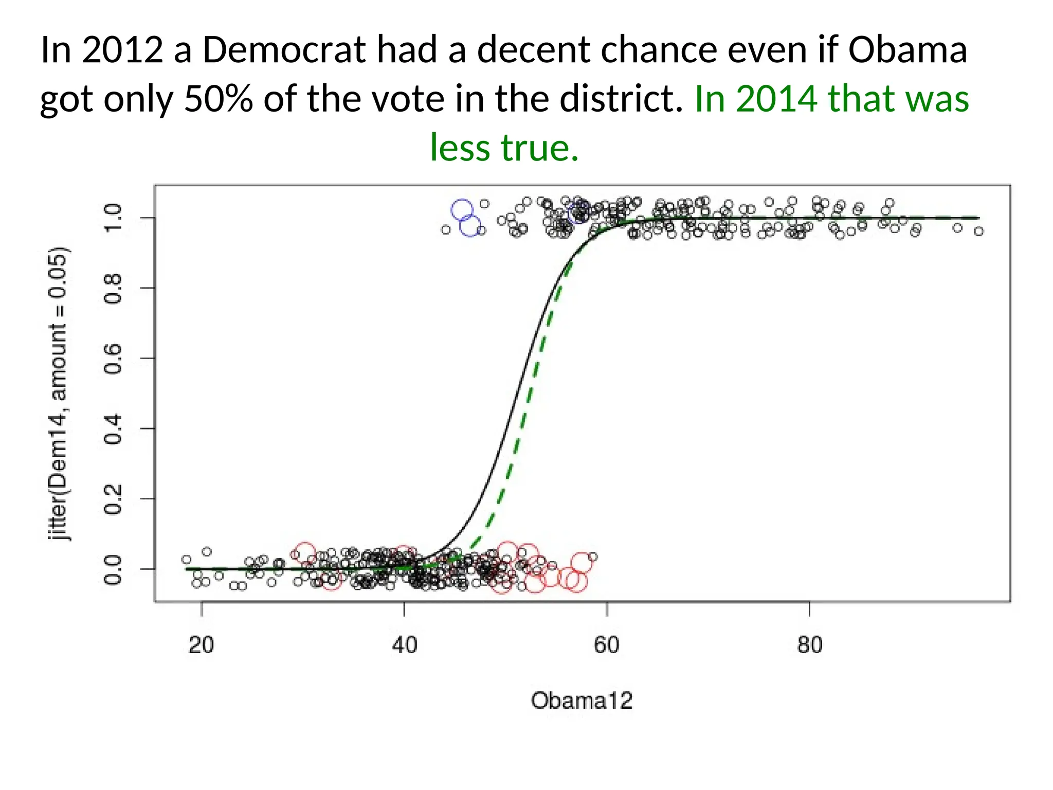
34. In 2012 a Democrat had a decent chance even if Obama
got only 50% of the vote in the district. In 2014 that was
less true.

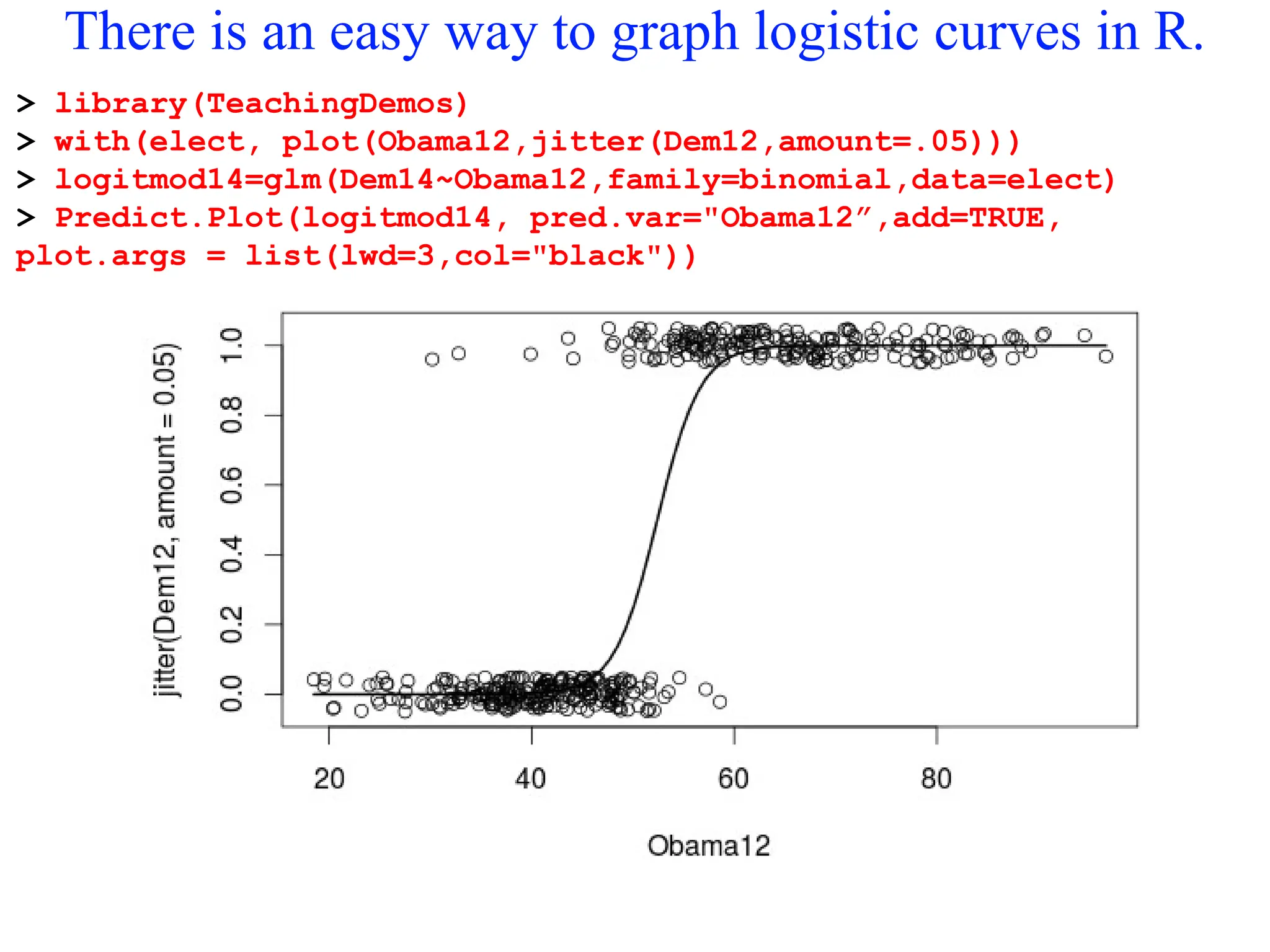
35. There is an easy way to graph logistic curves in R.
> library(TeachingDemos)
> with(elect, plot(Obama12,jitter(Dem12,amount=.05)))
> logitmod14=glm(Dem14~Obama12,family=binomial,data=elect)
> Predict.Plot(logitmod14, pred.var="Obama12”,add=TRUE,
plot.args = list(lwd=3,col="black"))

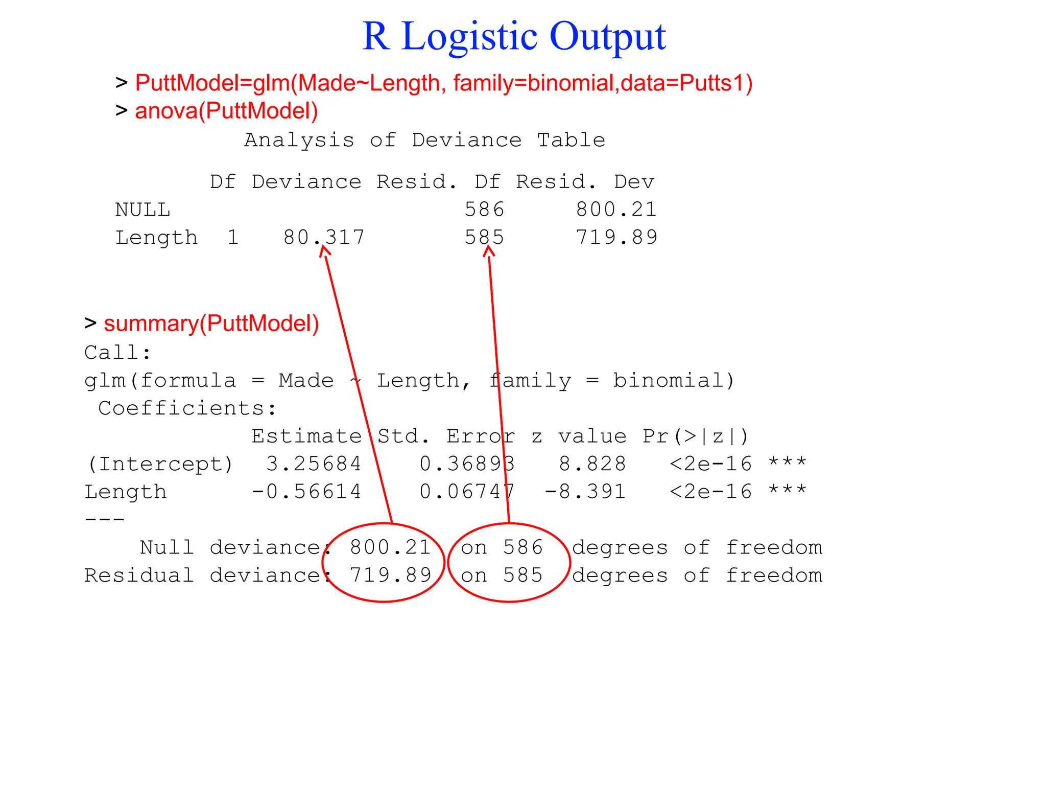
36. > summary(PuttModel)
Call:
glm(formula = Made ~ Length, family = binomial)
Coefficients:
Estimate Std. Error z value Pr(>|z|)
(Intercept) 3.25684 0.36893 8.828 <2e-16 ***
Length -0.56614 0.06747 -8.391 <2e-16 ***
---
Null deviance: 800.21 on 586 degrees of freedom
Residual deviance: 719.89 on 585 degrees of freedom
> PuttModel=glm(Made~Length, family=binomial,data=Putts1)
> anova(PuttModel)
Analysis of Deviance Table
Df Deviance Resid. Df Resid. Dev
NULL 586 800.21
Length 1 80.317 585 719.89
R Logistic Output

37. Two forms of logistic data
1. Response variable Y = Success/Failure or 1/0: “long
form” in which each case is a row in a spreadsheet
(e.g., Putts1 has 587 cases). This is often called
“binary response” or “Bernoulli” logistic regression.
2. Response variable Y = Number of Successes for a
group of data with a common X value: “short form”
(e.g., Putts2 has 5 cases – putts of 3 ft, 4 ft, … 7 ft).
This is often called “Binomial counts” logistic
regression.

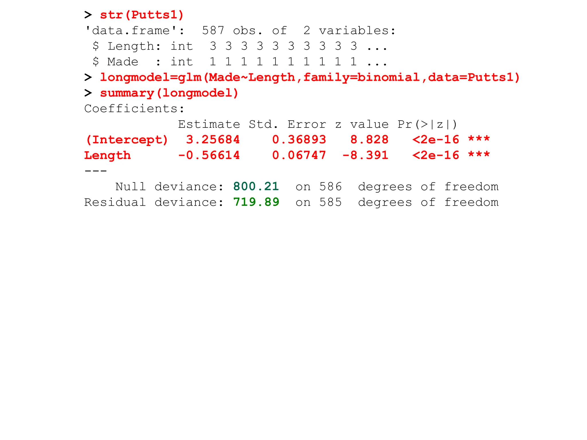
38. > str(Putts1)
'data.frame': 587 obs. of 2 variables:
$ Length: int 3 3 3 3 3 3 3 3 3 3 ...
$ Made : int 1 1 1 1 1 1 1 1 1 1 ...
> longmodel=glm(Made~Length,family=binomial,data=Putts1)
> summary(longmodel)
Coefficients:
Estimate Std. Error z value Pr(>|z|)
(Intercept) 3.25684 0.36893 8.828 <2e-16 ***
Length -0.56614 0.06747 -8.391 <2e-16 ***
---
Null deviance: 800.21 on 586 degrees of freedom
Residual deviance: 719.89 on 585 degrees of freedom

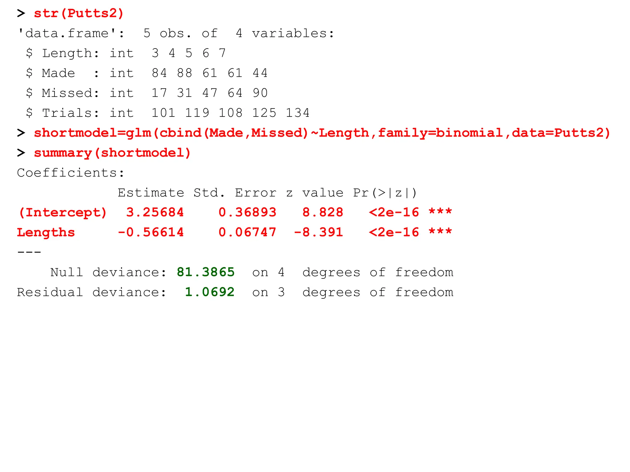
39. > str(Putts2)
'data.frame': 5 obs. of 4 variables:
$ Length: int 3 4 5 6 7
$ Made : int 84 88 61 61 44
$ Missed: int 17 31 47 64 90
$ Trials: int 101 119 108 125 134
> shortmodel=glm(cbind(Made,Missed)~Length,family=binomial,data=Putts2)
> summary(shortmodel)
Coefficients:
Estimate Std. Error z value Pr(>|z|)
(Intercept) 3.25684 0.36893 8.828 <2e-16 ***
Lengths -0.56614 0.06747 -8.391 <2e-16 ***
---
Null deviance: 81.3865 on 4 degrees of freedom
Residual deviance: 1.0692 on 3 degrees of freedom

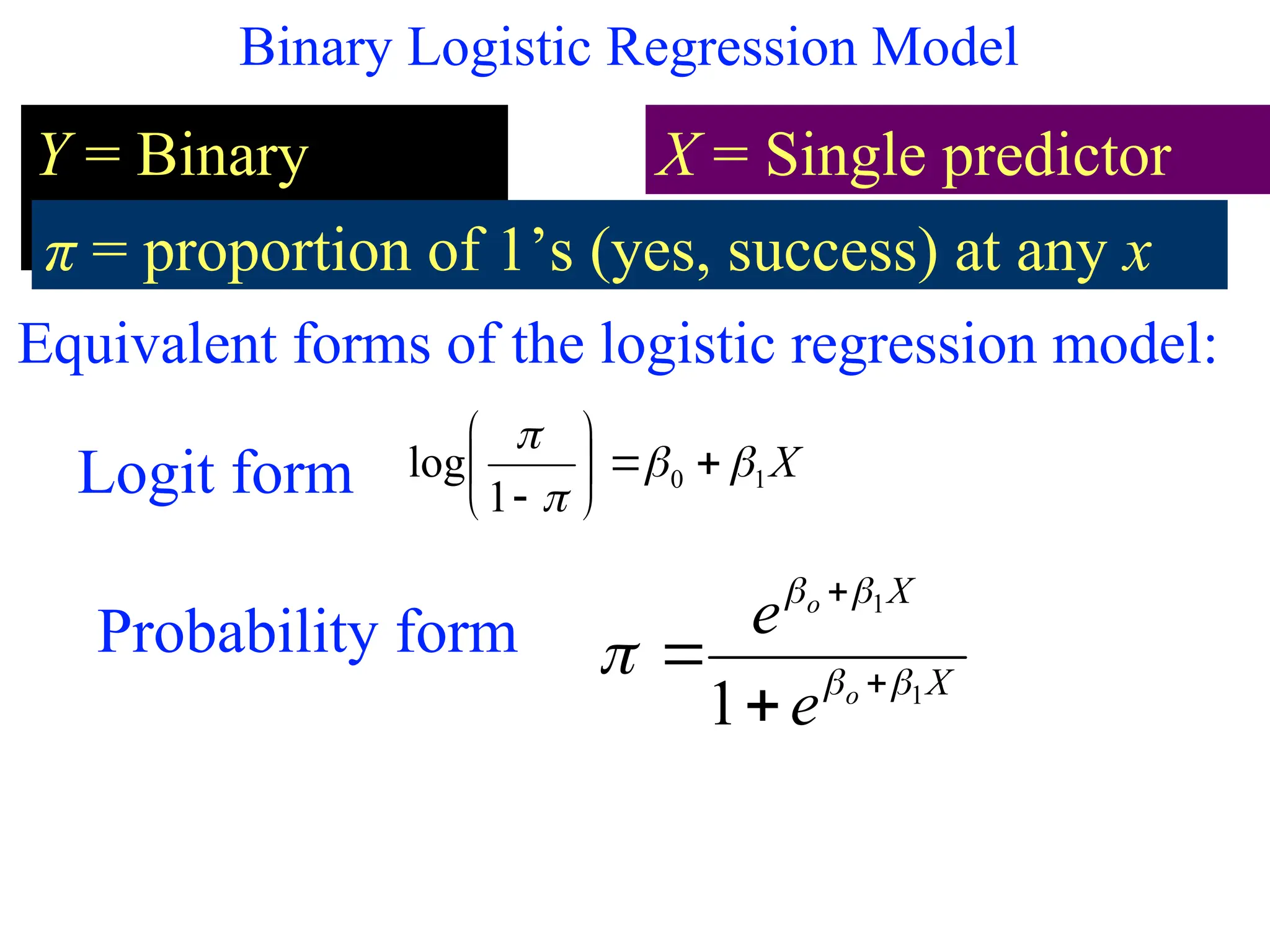
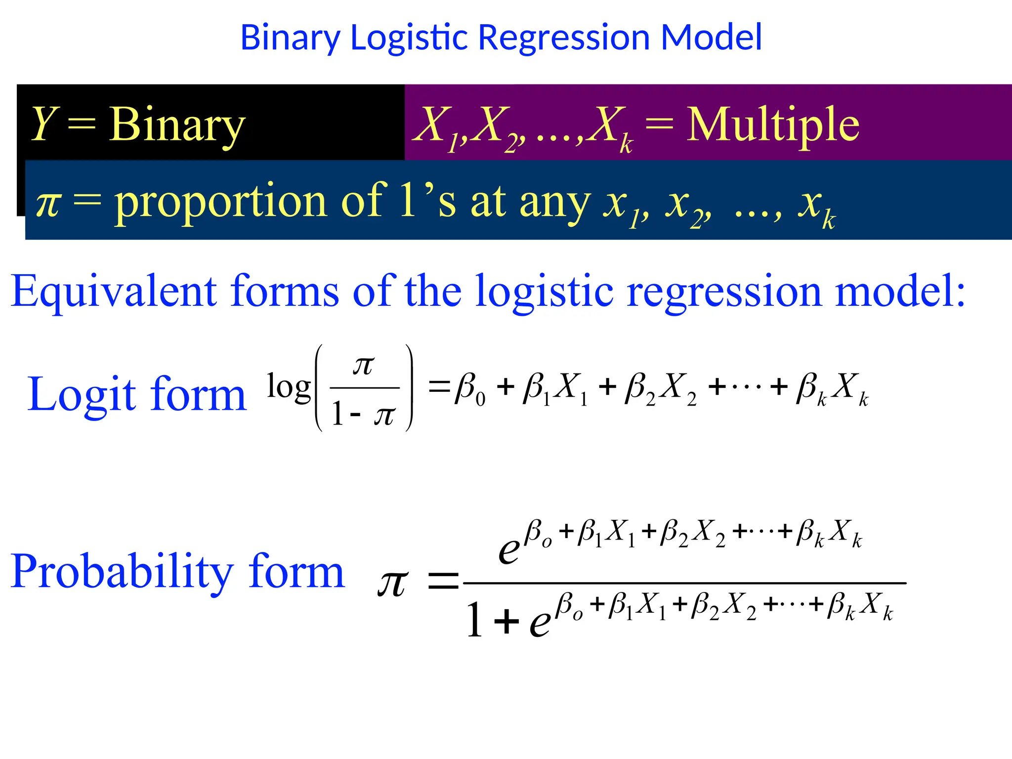
40. Binary Logistic Regression Model
Y = Binary
response
X = Single predictor
π = proportion of 1’s (yes, success) at any x
X
X
o
o
e
e
1
1
1 



 



Equivalent forms of the logistic regression model:
X
1
0
1
log 












Logit form
Probability form

41. Y = Binary
response
X = Single predictor
X
X
o
o
e
e
1
1
1 



 



X
1
0
1
log 












Logit form
Probability form
X1,X2,…,Xk = Multiple
predictors
π = proportion of 1’s (yes, success) at any x
π = proportion of 1’s at any x1, x2, …, xk
k
k X
X
X 


















2
2
1
1
0
1
log
k
k
o
k
k
o
X
X
X
X
X
X
e
e








 








 

2
2
1
1
2
2
1
1
1
Binary Logistic Regression Model
Equivalent forms of the logistic regression model:

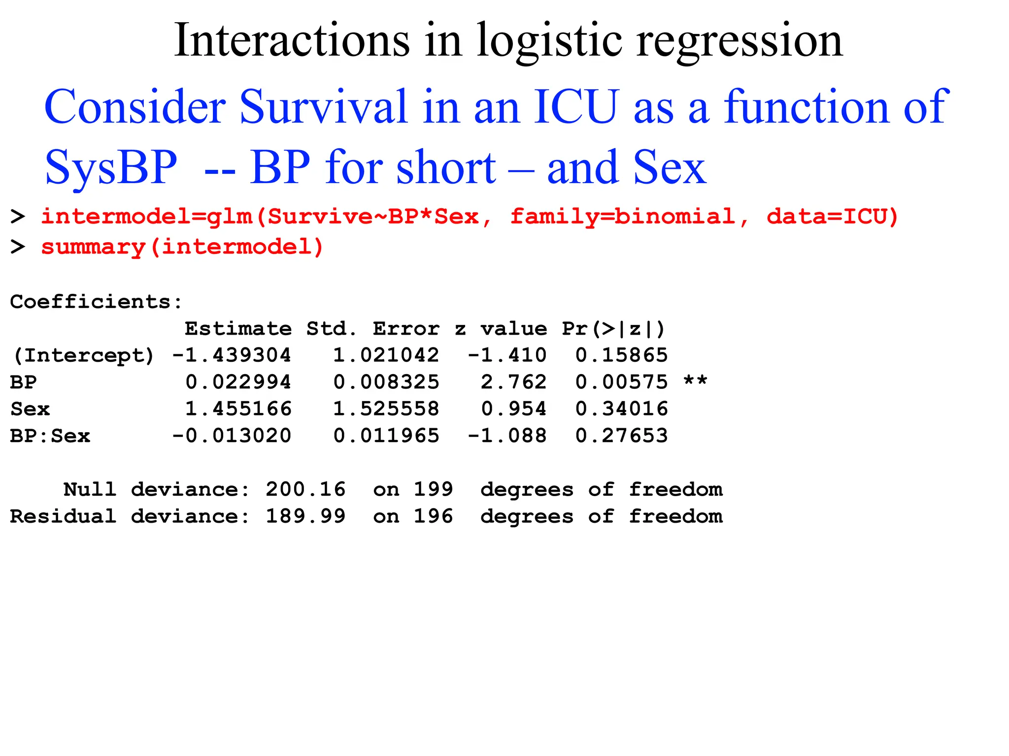
42. Interactions in logistic regression
Consider Survival in an ICU as a function of
SysBP -- BP for short – and Sex
> intermodel=glm(Survive~BP*Sex, family=binomial, data=ICU)
> summary(intermodel)
Coefficients:
Estimate Std. Error z value Pr(>|z|)
(Intercept) -1.439304 1.021042 -1.410 0.15865
BP 0.022994 0.008325 2.762 0.00575 **
Sex 1.455166 1.525558 0.954 0.34016
BP:Sex -0.013020 0.011965 -1.088 0.27653
Null deviance: 200.16 on 199 degrees of freedom
Residual deviance: 189.99 on 196 degrees of freedom

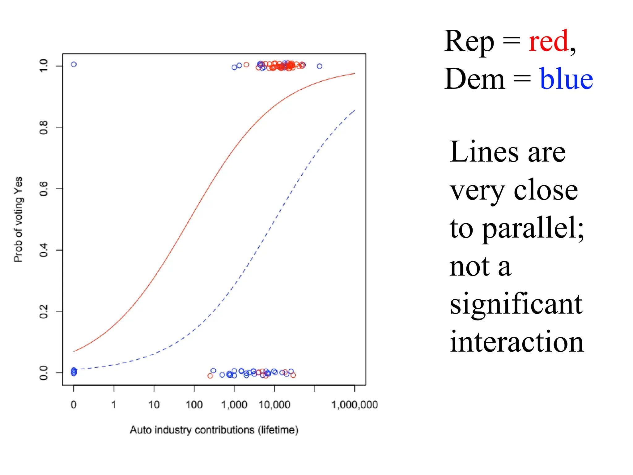
43. Rep = red,
Dem = blue
Lines are
very close
to parallel;
not a
significant
interaction

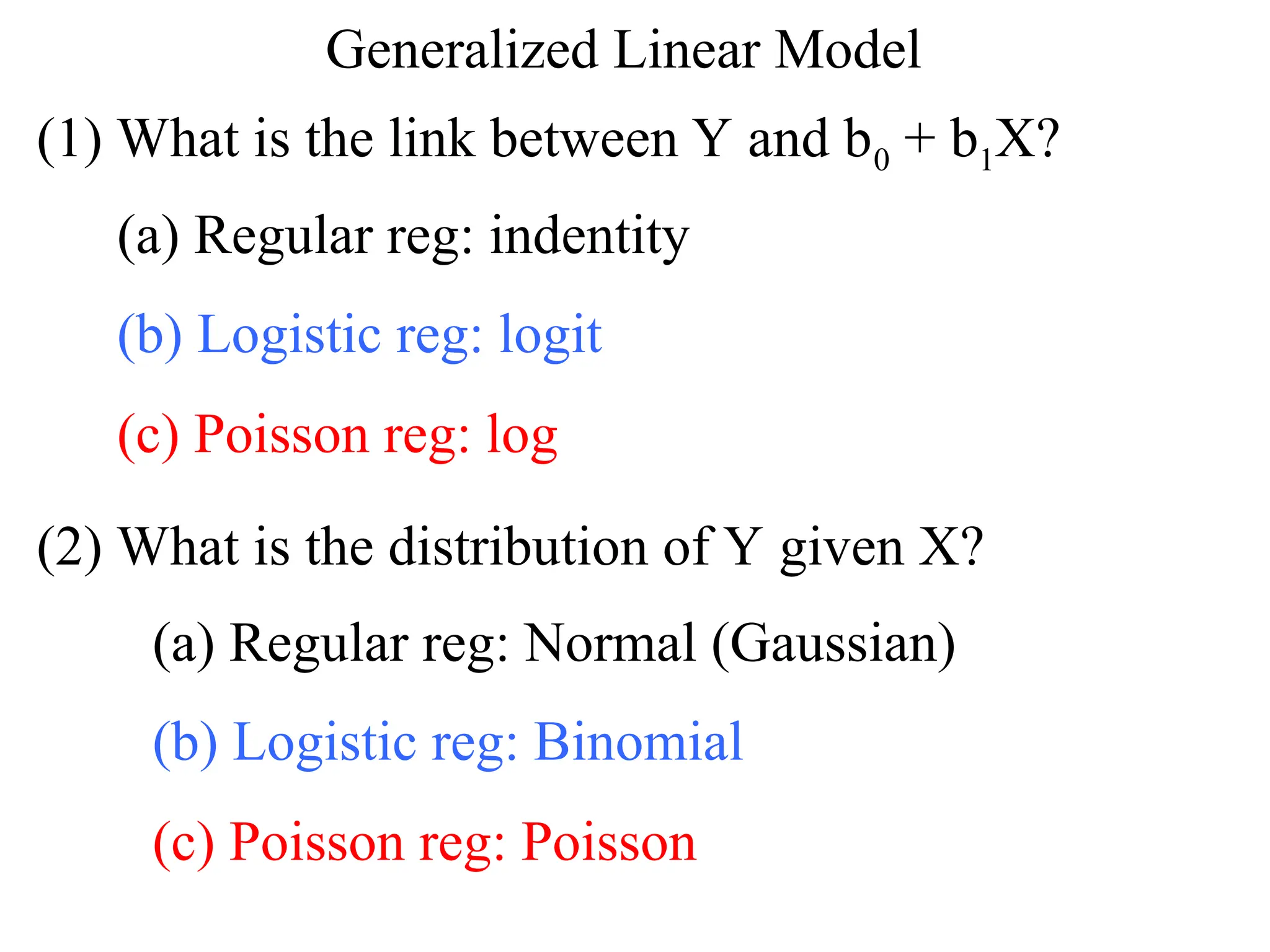
44. Generalized Linear Model
(1) What is the link between Y and b0 + b1X?
(2) What is the distribution of Y given X?
(a) Regular reg: indentity
(b) Logistic reg: logit
(c) Poisson reg: log
(a) Regular reg: Normal (Gaussian)
(b) Logistic reg: Binomial
(c) Poisson reg: Poisson

45. C-index, a measure of concordance
Med school acceptance: predicted by MCAT
and GPA?
Med school acceptance: predicted by coin toss??

46. > library(Stat2Data)
> data(MedGPA)
> str(MedGPA)
> GPA10=MedGPA$GPA*10
> Med.glm3=glm(Acceptance~MCAT+GPA10, family=binomial,
data=MedGPA)
> summary(Med.glm3)
> Accept.hat <- Med.glm3$fitted > .5
> with(MedGPA, table(Acceptance,Accept.hat))
Accept.hat
Acceptance FALSE TRUE
0 18 7
1 7 23
18 + 23 = 41 correct out of 55

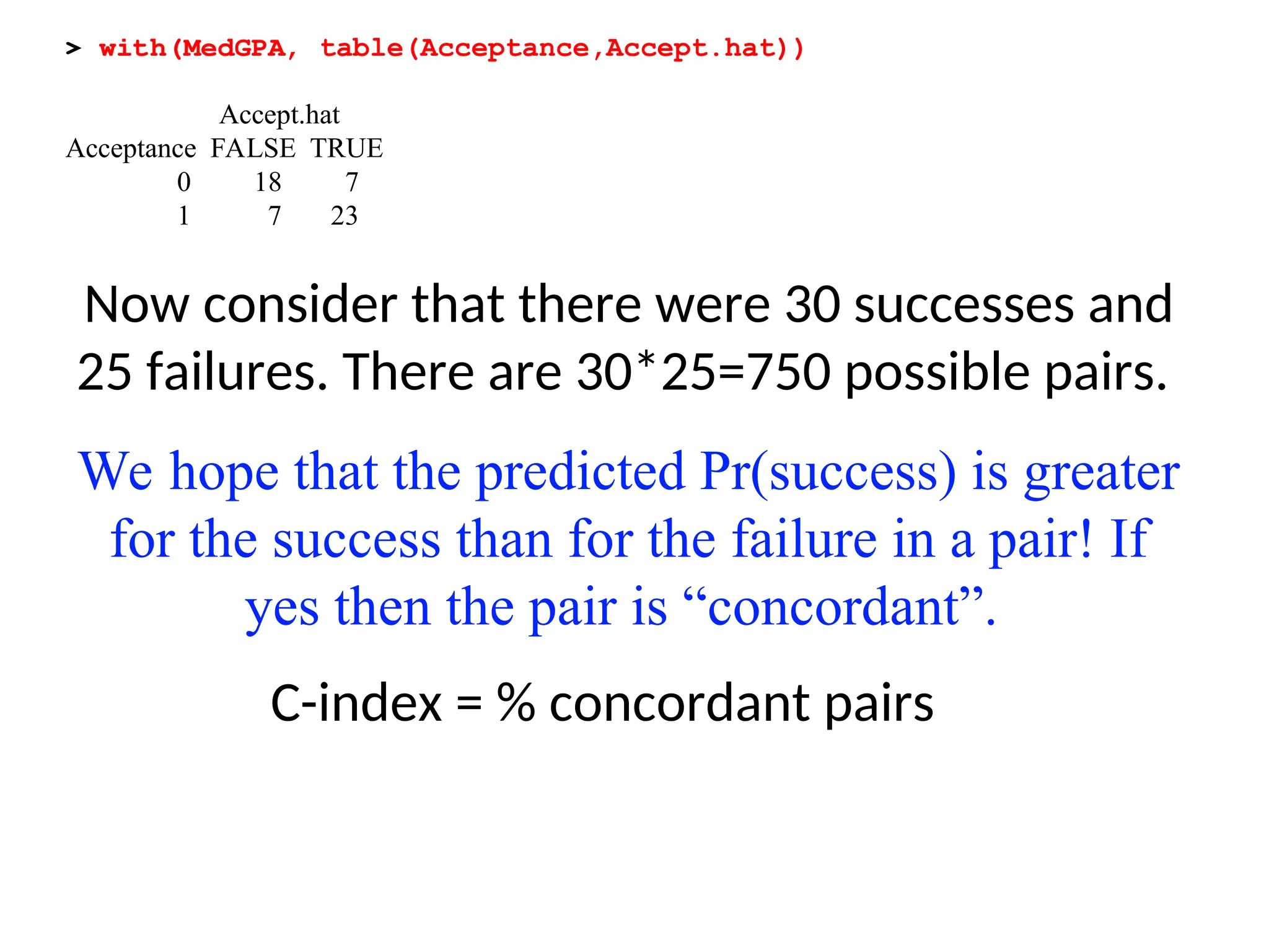
47. Now consider that there were 30 successes and
25 failures. There are 30*25=750 possible pairs.
We hope that the predicted Pr(success) is greater
for the success than for the failure in a pair! If
yes then the pair is “concordant”.
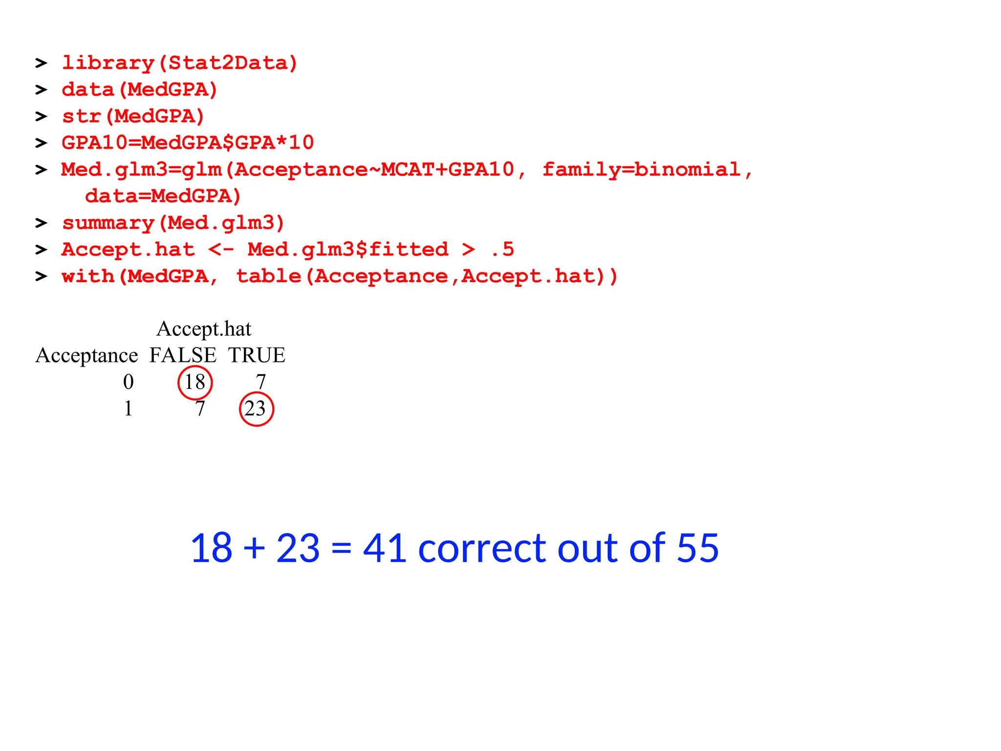
> with(MedGPA, table(Acceptance,Accept.hat))
Accept.hat
Acceptance FALSE TRUE
0 18 7
1 7 23
C-index = % concordant pairs

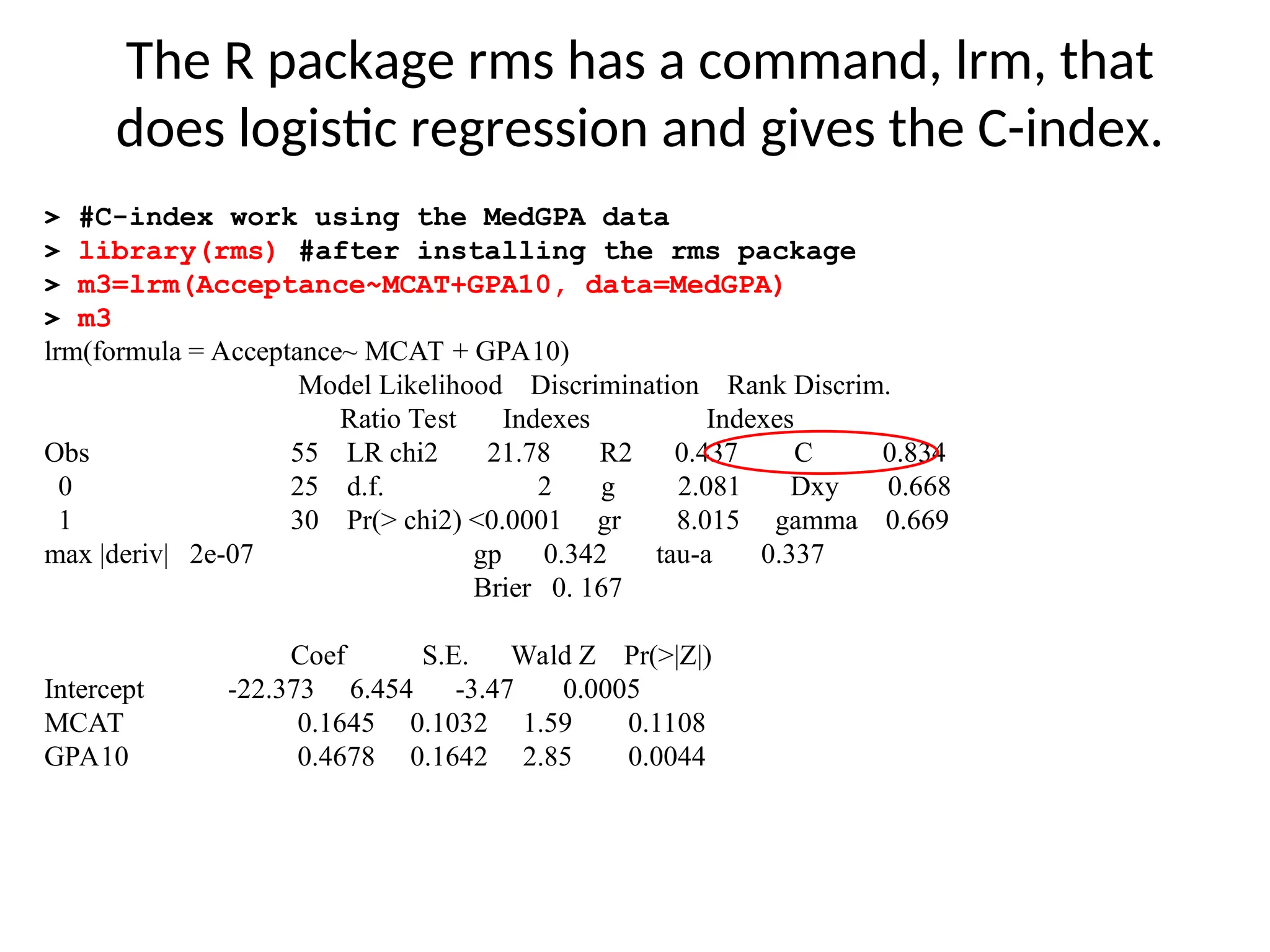
48. > #C-index work using the MedGPA data
> library(rms) #after installing the rms package
> m3=lrm(Acceptance~MCAT+GPA10, data=MedGPA)
> m3
lrm(formula = Acceptance~ MCAT + GPA10)
Model Likelihood Discrimination Rank Discrim.
Ratio Test Indexes Indexes
Obs 55 LR chi2 21.78 R2 0.437 C 0.834
0 25 d.f. 2 g 2.081 Dxy 0.668
1 30 Pr(> chi2) <0.0001 gr 8.015 gamma 0.669
max |deriv| 2e-07 gp 0.342 tau-a 0.337
Brier 0. 167
Coef S.E. Wald Z Pr(>|Z|)
Intercept -22.373 6.454 -3.47 0.0005
MCAT 0.1645 0.1032 1.59 0.1108
GPA10 0.4678 0.1642 2.85 0.0044
The R package rms has a command, lrm, that
does logistic regression and gives the C-index.

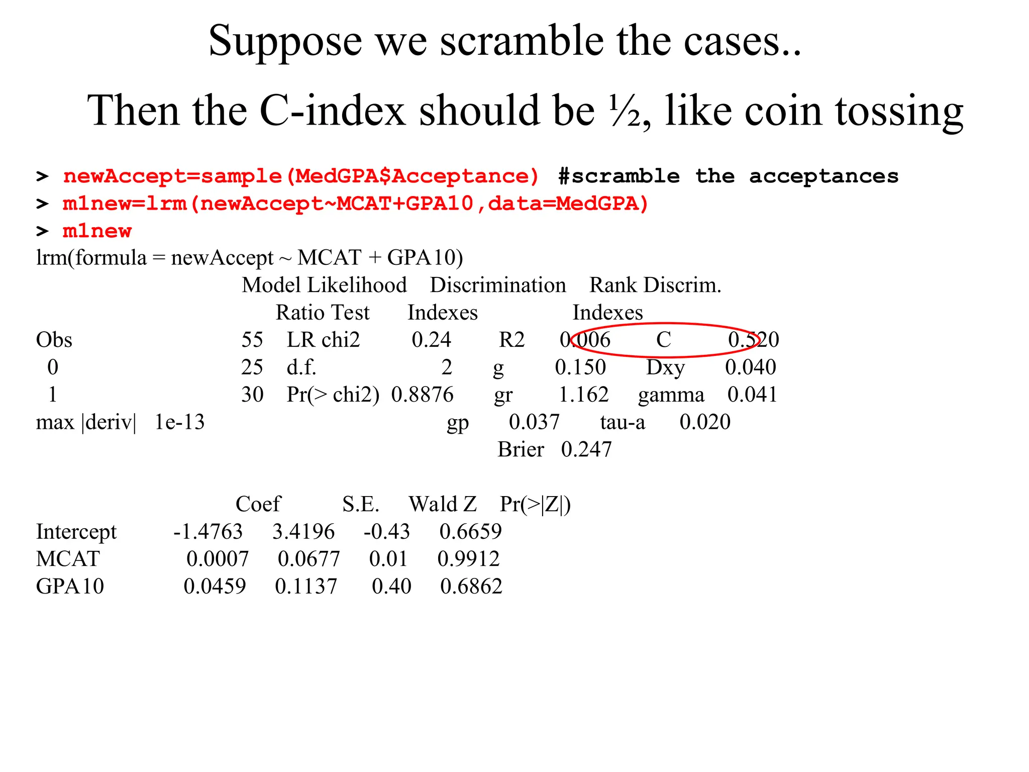
49. > newAccept=sample(MedGPA$Acceptance) #scramble the acceptances
> m1new=lrm(newAccept~MCAT+GPA10,data=MedGPA)
> m1new
lrm(formula = newAccept ~ MCAT + GPA10)
Model Likelihood Discrimination Rank Discrim.
Ratio Test Indexes Indexes
Obs 55 LR chi2 0.24 R2 0.006 C 0.520
0 25 d.f. 2 g 0.150 Dxy 0.040
1 30 Pr(> chi2) 0.8876 gr 1.162 gamma 0.041
max |deriv| 1e-13 gp 0.037 tau-a 0.020
Brier 0.247
Coef S.E. Wald Z Pr(>|Z|)
Intercept -1.4763 3.4196 -0.43 0.6659
MCAT 0.0007 0.0677 0.01 0.9912
GPA10 0.0459 0.1137 0.40 0.6862
Suppose we scramble the cases..
Then the C-index should be ½, like coin tossing