Befa file for ii mid exam

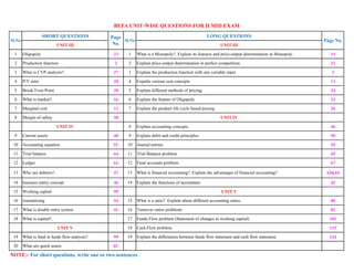
SHORT QUESTIONS LONG QUESTIONS
UNIT III UNIT III
1 Oligopoly 23 1 What is a Monopoly?. Explain its features and price-output determination in Monopoly. 19
2 Production function 2 2 Explain price-output determination in perfect competition. 22
3 What is CVP analysis?. 27 3 Explain the production function with one variable input 3
4 P/V ratio 28 4 Expalin various cost concepts 11
5 Break Even Point 28 5 Explain different methods of pricing. 24
6 What is market?. 16 6 Explain the feature of Oligopoly. 23
7 Marginal cost 13 7 Explain the product life cycle based pricing 26
8 Margin of safety 28 UNIT IV
UNIT IV 8 Explain accounting concepts. 46
9 Current assets 48 9 Explain debit and credit principles. 50
10 Accounting equation 51 10 Journal entries 55
11 Trial balance 64 11 Trial Balance problem 65
12 Ledger 61 12 Final accounts problem 67
13 Who are debtors?. 47 13 What is financial accounting?. Explain the advantages of financial accounting?. 42&44
14 business entity concept 46 14 Explain the functions of accountant. 42
15 Working capital 99 UNIT V
16 Journalizing 54 15 What is a ratio?. Explain about different accounting ratios. 80
17 What is double entry system 41 16 Turnover ratios problems 82
18 What is capital?. 17 Funds Flow problem (Statement of changes in working capital) 101
UNIT V 18 Cash Flow problem 115
19 What is fund in funds flow analysis?. 99 19 Explain the differences between funds flow statement and cash flow statement. 124
20 What are quick assets 81
BEFA UNIT-WISE QUESTIONS FOR II MID EXAM
Page No.Sl.No Sl.No
NOTE:- For short questions, write one or two sentences.
Page
No.

BEFA UNIT III
PRODUCTION
Production is the transformation or conversion of resources into commodities over time. Economists view
production as an activity through which utility is created or enhanced for a product. A firm is a business unit
which undertakes the activity of transforming inputs into output of goods and services.
FACTORS OF PRODUCTION
Factors of production is an economic term that describes the inputs that are used in the production of goods or
services in order to make an economic profit. The factors of production include land, labor, capital and
entrepreneurship. These production factors are also known as management, machines, materials and labor, and
knowledge has recently been talked about as a potential new factor of production.
1. Land
Land is short for all the natural resources available to create supply. It includes raw land and anything that
comes from the land. It can be a non-renewable resource.
That includes commodities such as oil and gold. It can also be a renewable resource, such as timber. Once man
changes it from its original condition, it becomes a capital good. For example, oil is a natural resource, but
gasoline is a capital good. Farmland is a natural resource, but a shopping center is a capital good.
The income earned by owners of land and other resources is called rent.
2. Labour
Labor is the work done by people. The value of labor depends on workers' education, skills, and motivation. It
also depends on productivity. That measures how much each hour of worker time produces in output.
The reward or income for labor is wages.
3. Capital
Capital is short for capital goods. These are man-made objects like machinery, equipment, and chemicals, that
are used in production. That's what differentiates them from consumer goods. For example, capital goods
include industrial and commercial buildings, but not private housing. A commercial aircraft is a capital good
but a private jet is not.
The income earned by owners of capital goods is called interest.
4. Entrepreneurship
1

BEFA UNIT III
Q = Output
f = Function of
L1 = Land
L2 = Labour
C = Capital
O = Organization
T = Technology
Entrepreneurship is the drive to develop an idea into a business. An entrepreneur combines the other three
factors of production to add to supply. The most successful are innovative risk-takers.
The income entrepreneurs earn is profits.
PRODUCTION FUNCTION
The production function expresses a functional relationship between physical inputs and physical outputs of a
firm at any particular time period. The output is thus a function of inputs. So, production function is an input –
output relationship. Mathematically production function can be written as
Q= f (L1,L2 C,O,T)
Here output is the function of inputs. Hence output becomes the dependent variable and
inputs are the independent variables.
Definition :
Samueson defines the production function as “The technical relationship which reveals the maximum
amount of output capable of being produced by each and every set of inputs”
Michael R Baye defines the production function as” That function which defines the maximum amount
of output that can be produced with a given set of inputs.”
Assumptions:
Production function has the following assumptions.
1. The production function is related to a particular period of time.
2. There is no change in technology.
3. The producer is using the best techniques available.
4. The factors of production are divisible.
5. Production function can be fitted to a short run or to long run.
2

BEFA UNIT III
PRODUCTION FUNCTION WITH ONE VARIABLE INPUT
The law of variable proportions which was earlier called as “Law of diminishing returns has
played a vital role in the modern economics theory. Assume that a firms‟ production function consists of fixed
quantities of all inputs (land, equipment, etc.) except labour which is a variable input. If you go on adding the
variable input, say, labor, the total output in the initial stages will increase at an increasing rate, and after
reaching certain level of output the total output will increase at declining rate. If variable factor inputs are added
further to the fixed factor input, the total output may decline. This law is of universal nature and it proved to be
true in agriculture.
Assumptions of the Law: The law is based upon the following assumptions:
1. Only one factor is varied
2. The scale of output is unchanged
3. The technique of production is unchanged
4. All units of factor input varied are homogeneous
Three stages of law:
The behaviour of the Output when the varying quantity of one factor is combined with a fixed quantity of the
other can be divided in to three district stages. The three stages can be better understood by following the table.
3

BEFA UNIT III
From the above graph the law of variable proportions operates in three stages. In the first stage,
total product increases at an increasing rate. The marginal product in this stage increases at an increasing rate
resulting in a greater increase in total product. The average product also increases. This stage continues up to
the point where average product is equal to marginal product. The law of increasing returns is in operation at
this stage. The law of diminishing returns starts operating from the second stage onwards. At the second stage
total product increases only at a diminishing rate. The average product also declines. The second stage comes to
an end where total product becomes maximum and marginal product becomes zero. The marginal product
becomes negative in the third stage. So the total product also declines. The average product continues to
decline.
We can sum up the above relationship thus when „AP‟ is rising, “MP‟ rises more than “AP; When „AP” is
maximum and constant, „MP‟ becomes equal to „AP‟ when „AP‟ starts falling, „MP‟ falls faster than „AP‟.
Thus, the total product, marginal product and average product pass through three phases, viz., increasing
diminishing and negative returns stage. The law of variable proportion is nothing but the combination of the law
of increasing and demising returns.
PRODUCTION FUNCTION WITH TWO VARIABLE INPUTS
Isoquants analyse and compare the different combinations of capital & labour and output. The term isoquant
has its origin from two words “iso” and “quantus”. „iso‟ is a Greek word meaning „equal‟ and „quantus‟ is a
Latin word meaning „quantity‟. Isoquant therefore, means equal quantity. An isoquant curve is therefore called
as iso-product curve or equal product curve or production indifference curve.
Thus, an isoquant shows all possible combinations of two inputs, which are capable of producing equal or a
given level of output. Since each combination yields same output, the producer becomes indifferent towards
these combinations.
Assumptions:
1. There are only two factors of production, viz. labour and capital.
2. The two factors can substitute each other up to certain limit
3. The shape of the isoquant depends upon the extent of substitutability of the two inputs.
4. The technology is given over a period.
For example:- Now the firm can combine labor and capital in different proportions and can maintain specified
level of output say, 10 units of output of a product X. It may combine alternatively as follows:
In the below table, combination „A‟ represent 1 unit of capital and 10 units of labour and produces „10‟ units of
a product. All other combinations in the table are assumed to yield the same given output of a product say „10‟
units by employing any one of the alternative combinations of the two factors labour and capital. If we plot all
these combinations on a paper and join them, we will get a curve called Iso-quant curve as shown below.
4

BEFA UNIT III
Labour is on the X-axis and capital is on the Y-axis. IQ is the Iso-Quant curve which shows all the alternative
combinations A, B, C, D which can produce 10 units of a product.
Features of an ISOQUANT:
1. Downward sloping:-If one of the inputs is reduced, the other input has to be
increased. There is no question of increase in both the inputs to yield a given output.
2. Don’t touch the axes:- The isoquant touches neither X-axis nor Y-axis, as both inputs
are required to produce a given product.If an isoquant is touching the X-axis, it means
output is possible even by using a factor(Ex: Labor alone without using capital). But,
this is unrealistic.
3. Don’t intersect:- Iso-quants representing different levels of output never intersect or
touch or be tangent to each other. If they intersect to each other, they have a common
point on them which means that the same amount of labor and capital produce two
different levels of output.
4. Convex to origin:-Isoquants are convex to the origin. It is because the inputs factor
are not perfect substitutes. One input factor is substituted by other input factor in a
decreasing marginal rate.The convexity of isoquant suggests that MRTS is diminishing
which means that as quantities of one factor-labor is increased , the less of another
factor-capital will be given up, if output level is to be kept constant.
5. Upper isoquants represent higher level of output:- Each isoquant represents a
different quantity of output. Higher isoquants indicate a higher level of output.
LAW OF RETURNS TO SCALE
The concept of variable proportions is a short-run phenomenon as in these period fixed
factors cannot be changed and all factors cannot be changed. On the other hand in the long-term all factors can
be changed as made variable. When we study the changes in output when all factors or inputs are changed, we
5

BEFA UNIT III
study returns to scale. An increase in the scale means that all inputs or factors are increased in the same
proportion. In variable proportions, the cooperating factors may be increased or decreased and one faster (Ex.
Land in agriculture (or) machinery in industry) remains constant so that the changes in proportion among the
factors result in certain changes in output. In returns to scale, all the necessary factors or production are
increased or decreased to the same extent so that whatever the scale of production, the proportion among the
factors remains the same.
Assumptions
1. Technique of production is unchanged
2. All units of factors are homogeneous
3. Returns are measured in physical terms
When a firm expands, its scale increases all its inputs proportionally, then technically there are three
possibilities.
1. Law of increasing returns to scale:- if a proportionate/percentage increase
in the output is larger than the proportionate/percentage increase in inputs, there
are increasing returns.
For example: If a 5% increase in inputs, results in 10% increase in the
output, a firm is said to attain increased returns.
If PFC > 1, it means increasing returns to scale
If PFC = 1, it means constant returns to scale
If PFC < 1, it means decreasing returns to scale
2. Law of constant returns to scale:- if the proportionate increase in all the inputs
is equal to the proportionate increase in output, then situation of constant returns to
scale occurs.
For Example:- If the inputs are increased at 10% and if the resultant output also
increases a 10% then the organization is said to achieve constant returns to scale.
3. Law of decreasing returns to scale:- if the proportionate increase in output is
less than the proportionate increase in input, then a situation of decreasing returns
to scale occurs.
For Example:- If the inputs are increased by 10% and if the resultant output
increases only by 5% then the organization is said to achieve decreasing returns to
6

BEFA UNIT III
Q = Total production/Output
a = Total factor productivity/Multi -factor productivity
(The ratio of output to the sum of associated labor and capital
inputs). Productivity is measure of efficiency of labor/machines etc, in
converting input into output.
L = Index of employment of labor = Labour units
K = Index of employment of capital = Capital units
b = Output elasticity of labor (1% change in labor results in b% change
in output)
c = Output elasticity of capital (1% change in capital results in c% change
in output)
𝐅𝐚𝐜𝐭𝐨𝐫 𝐩𝐫𝐨𝐝𝐮𝐜𝐭𝐢𝐯𝐢𝐭𝐲 =
𝐎𝐮𝐩𝐮𝐭
𝐅𝐚𝐜𝐭𝐨𝐫 𝐢𝐧𝐩𝐮𝐭
𝐓𝐨𝐭𝐚𝐥 𝐅𝐚𝐜𝐭𝐨𝐫 𝐏𝐫𝐨𝐝𝐮𝐜𝐭𝐢𝐯𝐢𝐭𝐲 =
𝐓𝐨𝐭𝐚𝐥 𝐎𝐮𝐩𝐮𝐭
𝐓𝐨𝐭𝐚𝐥 𝐢𝐧𝐩𝐮𝐭𝐬
scale.
the following table illustrates these laws clearly.
From the above table it is clear that with 1 unit of capital and 3 units of labor, the firm produces 50 units of
output. When the inputs are doubled 2 units of capital and 6 units of labor, the output has gone up to 120 units.
Thus when inputs are increased by 100%, the output has increased by 140%. That is , output has increased by
more than double. This is governed by law of increasing returns to scale.
When the inputs are further doubled that is to 4 units of capital and 12 units of labor, the output has gone to 240
units. Thus, when inputs are increased by 100%., the output has increased by 100%. That is, output has
doubled. This governed by law of constant returns to scale.
When the inputs further doubled, that is, to 8 units of capital and 24 units of labor, the output has gone up to
360 units. Thus, when inputs are increased by 100%, the output has increased by only 50%. This is governed by
law of decreasing returns to scale.
DIFFERENT TYPES OF PRODUCTION FUNCTIONS
1. Cobb-Douglas Production Function
This production function was proposed by C. W. Cobb and P. H. Dougles. This famous statistical
production function is known as Cobb-Douglas production function. Originally the function is applied on the
empirical study of the American manufacturing industry from 1899 to 1922. Cobb – Douglas production
function takes the following
mathematical form.
Q = aLb
KC
Q = 1.01L0.75
K0.25
The above production function shows
that 1% change in labor input, capital
remaining the same, is associated with a
0.75 percent change in output.
Similarly, 1% change in capital, labor remaining the same, is associated with a 0.25 percent change in output.
7

BEFA UNIT III
Assumptions:
It has the following assumptions
1. The function assumes that output is the function of two factors viz. capital and labour.
2. It is a linear homogenous production function of the first degree
3. There are constant returns to scale b+c=1
4. All inputs are homogenous
5. There is perfect competition
6. There is no change in technology
7. Both L&K should be positive for to Q to exist. If either of these is zero, Q will be zero. This implies
that both labor and capital will be combined to get output.
2. Leontief Production Function:
Leontief production function, also known as Fixed Proportion Production Function, uses fixed proportion of
inputs having no substitutability between them. It is regarded as the limiting case for constant elasticity of
substitution.
The production function can be expressed as follows:
Where, q = quantity of output produced
Z1 = utilized quantity of input 1
Z2 = utilized quantity of input 2
a and b = constants
For example, tyres and steering wheels are used for producing cars. In such a case, the production function can
be as follows:
Q = min (z1/a, Z2/b)
Q = min (number of tyres used, number of steering wheels used).
8

BEFA UNIT III
Suppose that the inputs "tires" and "steering wheels" are used in the production of a car (for simplicity of the
example, to the exclusion of anything else). Then in the above formula q refers to the number of cars produced
i.e., one in our example, z1 refers to the number of tires used, and z2 refers to the number of steering wheels
used. Assuming that each car is produced with 4 tires and 1 steering wheel, the Leontief production function is
Number of cars = Min{¼ times the number of tires, 1 times the number of steering wheels}.
In the above given figure, OR shows the fixed Tyres-Wheels ratio, if a firm wants to produce 1 car, then 4 tyres
and 1 wheel must be used.
Similarly, for the production of 3 cars and 4 cars, 12 tyres and 3 wheel and 16 tyres and 4 wheel must be
employed respectively.
3. CES Production Function
Definition: The Constant Elasticity of Substitution Production Function or CES implies, that any change in
the input factors, results in the constant change in the output. In CES, the elasticity of substitution is constant
and may not necessarily be equal to one or unity.
In constant elasticity of substitution production function, all the input factors are taken into the consideration
such as raw material, technology, labor, capital, etc. The marginal product of one factor increases with the
increase in the value of the other factors of production. Also, the marginal product of labor and capital will be
positive in case of constant returns to scale.
The constant elasticity of substitution production function can be expressed algebraically as:
𝑸 = 𝑨[𝜶𝑲−𝜷
+ 𝟏 − 𝜶 𝑳−𝜷
]−𝟏/𝜷
Where, Q = output, K = Capital and L = Labor
A = efficiency parameter that shows the organizational aspects of production and the state of technology.
The Constant elasticity of substitution production function shows, that any change in the technology or
organizational aspects, the production function changes with a shift in the efficiency parameter.
9

BEFA UNIT III
α= distribution parameter or capital intensity factor coefficient concerned with relative factors in the total
output.
β = substitution parameter, that determines the elasticity of substitution
The homogeneity of the production function can be determined by the value of the substitution parameter (β), if
it is equal to one, then it is said to be linearly homogeneous i.e. the proportionate change in the input factors
results in the increase in the output in the same proportion.
The homogeneity of the production function can be determined by the value of the substitution parameter (β), if
it is equal to one, then it is said to be linearly homogeneous i.e. the proportionate change in the input factors
results in the increase in the output in the same proportion.
For example:
Consider the following production function.
Q = 5K + 10L
It means 1 unit K produces 5 units and 2 units of L produce 10 units.
If we assume that, initially K = 1, L = 2, the total output may be obtained by substituting 1 for K and 2 for L in
the below equation. Thus,
Qx1 = 5(1) + 10(2)
25 = 5 + 20
when inputs are doubled (i.e., K =2 and L = 4). Then,
Qx2 = 5(1x2) + 10(2x2)
50 = 10 + 40
Thus, the given production functions, when inputs are doubled, the output is also doubled.
10

BEFA UNIT III
TYPES OF COSTS
Profits are the difference between selling price and cost of production. In general the selling price is not within
the control of a firm but many costs are under its control. The firm should therefore aim at controlling and
minimizing cost. The various relevant concepts of cost are:
1. Opportunity costs and Outlay costs:
Opportunity costs refer to the „costs of the next best alternative foregone‟. We have scarce resources
and all these have alternative uses. Where there is an alternative, there is an opportunity to reinvest the
resources. In other words, if there are no alternatives, there are no opportunity costs. It is necessary that we
should always consider the cost of the next best alternative foregone before committing the funds on a given
option. In other words, the benefits from the present option should be more than the benefits of the next best
alternative. Opportunity cost is said to exist when the resources are scarce and there are alternative uses for
these resources. If there is no alternative, Opportunity cost is zero.
For example: if a firm owns a land, there is no cost of using the land (i.e., the rent) in firm‟s account.
Bust the firm has an opportunity cost of using this land, which is equal to the rent foregone by not letting the
land out on (the return of second best alternative is regarded as the cost of first best alternative) rent.
Out lay costs are as actual costs which are actually incurred by the firm. these are the payments made
for labour, material, plant, building, machinery traveling, transporting etc., These are all those expenses
appearing in the books of account, hence based on accounting cost concept.
2. Explicit costs and Implicit costs:
Explicit costs are also called as out-of-pocket cost that involve cash payments. These are the actual or
business costs that appear in the books of accounts. These costs include payment of wages and salaries,
payment for raw-materials, interest on borrowed capital funds, rent on hired land, Taxes paid etc.
Implicit costs are also called as imputed costs which don‟t involve payment of cash as they are not
actually incurred. They would have been incurred had the owner not been in possession of the facilities. Ex:
Interest on own capital, saving in terms of salary due to own supervision and rent of own building etc.
3. Historical costs and Replacement costs:
Historical cost is the original cost that has been originally spent to acquire the asset. of an asset.
Historical valuation is the basis for financial accounts.
A replacement cost is the price that is to be paid currently to replace the same asset. A replacement cost
is a relevant cost concept when financial statements have to be adjusted for inflation.
4. Short – run costs and Long – run costs:
Short-run is a period during which the physical capacity of the firm remains fixed. Any increase in
output during this period is possible only by using the existing physical capacity more extensively. So short run
cost is that which varies with output when the plant and capital equipment are constant.
11

BEFA UNIT III
Long run is defined as a period of adequate length during which a company may alter all factors of
production with high degree of flexibility.
5. Out-of pocket costs and Books costs:
Out-of pocket costs also known as explicit costs are those costs that involve current cash payment
such as purchase of raw material, payment of salary rents payment, interest on loan etc.
Book costs also called implicit costs do not require current cash payments. Depreciation, unpaid
interest, salary of the owner is examples of back costs.
6. Fixed costs, Variable costs and Semi-variable costs:
Fixed cost is that cost which remains constant for a certain level to output. It is not affected by the
changes in the volume of production but fixed cost per unit decreases, when the production is increased. Fixed
cost includes salaries, Rent, Administrative expenses depreciations etc.
Variable is that which varies directly with the variation in output. An increase in total output results in
an increase in total variable costs and decrease in total output results in a proportionate deccease in the total
variables costs. The variable cost per unit will be constant. Ex: Raw materials, labour, direct expenses, etc.
Semi-variable costs refer to such costs that are fixed to some extent beyond which they are variable. Ex:
telephone charges, Electricity charges, etc.
7. Past costs and Future costs:
Past costs also called historical costs are the actual cost incurred and recorded in the book of account
these costs are useful only for valuation and not for decision making.
Future costs are costs that are expected to be incurred in the futures. They are not actual costs. They are
the costs forecasted or estimated with rational methods. Future cost estimate is useful for decision making
because decision are meant for future.
8. Separable costs and Joint costs:
The costs which can be traced or identified directly with a particular unit, department, or a process of
production are called separable costs or direct costs or traceable costs.
The costs which cannot be identified directly with a particular unit, department or a process of the
production are called joint costs or indirect costs or common costs. These costs are apportioned among various
departments. Ex: Rent, Electricity, Administration salaries, Research and Development expenses etc.
9. Avoidable costs and Unavoidable costs:
Avoidable costs are those costs, which can be reduced if the business activities of a concern are
curtailed. For example, if some workers can be retrenched with a drop in production, the wages of the
retrenched workers are escapable costs.
12

BEFA UNIT III
Unavoidable costs are those that are essential for the sustenance of the business activity and hence they
have to be incurred.
10. Controllable costs and Uncontrollable costs:
Controllable costs are ones, which can be regulated by the executive who is in charge of it. Direct
expenses like material, labour etc. are controllable costs.
Some costs are not directly identifiable with a process of product. They are apportioned to various
processes or products in some proportion. These apportioned costs are called uncontrollable costs.
11. Incremental costs and Sunk costs:
Incremental cost also known as differential cost is the additional cost due to a change in the level or
nature of business activity. The change may be caused by adding a new product, adding new machinery,
replacing a machine by a better one etc.
Sunk costs are those which are not altered by any change – They are the costs incurred in the past. This
cost is the result of past decision, and cannot be changed by future decisions. Investments in fixed assets are
examples of sunk costs. Once an asset is bought, the funds are blocked forever. They can neither be changed
nor controlled.
12. Total costs, Average costs and Marginal costs:
Total cost is the total expenditure incurred for the input needed for production. It may be explicit or
implicit. It is the sum total of the fixed and variable costs.
Average cost is the cost per unit of output. It is obtained by dividing the total cost (TC) by the total
quantity produced (Q)
Marginal cost is the additional cost incurred to produce an additional unit of output.
13. Accounting costs and Economic costs:
Accounting costs are the costs recorded for the purpose of preparing the profit & loss account and
balance sheet to meet the legal, financial and tax purpose of the company. The accounting concept is a historical
concept and records what has happened in the post.
Economic cost refers to cost of economic resources used in production including opportunity cost.
Economics concept considers future costs and future revenues, which help future planning, and choice, while
the accountant describes what has happened, the economics aims at projecting what will happen.
14. Urgent costs and Postponable costs:
Urgent cost are those costs such as raw materials, wages and son, necessary to sustain the productivity.
Postponable costs are those costs which can be conveniently postponed. For example, white washing
the building etc.
13

BEFA UNIT III
COST-OUTPUT RELATIONSHIP
The cost-output relationship plays an important role in determining the optimum level of production.
Knowledge of the cost-output relationship helps the manager in cost control, profit prediction, pricing,
promotion etc. Output is an important factor, which influences the cost. Considering the period the cost function
can be classified as (a) short-run cost function and (b) long-run cost function. In the short run, the costs can be
classified into fixed costs and variable costs. The cost-output relationship in the short run is governed by certain
restrictions in terms of fixed costs whereas in the long run, the cost-output relationship studies the effect of
varying the size of plants upon its cost.
I. Short-run Cost Function:
Under short run cost-output relation, costs in short run are classified into fixed costs and variable costs.
Labour is the variable factor while capital is the fixed factor. Total fixed cost remains constant while variable
cost changes with the variation in units if labour. The fixed costs may be ascertained in terms of total fixed cost
and average fixed cost per unit. The variable cost can be determined in terms of average variable cost, total
variable cost. The below table explains the behavior of costs in the short run. From the below it is clear that:
 Total fixed costs remain fixed irrespective of increase or decrease in production activity.
 Average fixed cost per unit declines as the volume of production increases. As production increases, the
fixed costs are spread over a great number of units. There is inverse relationship between average fixed
cost and volume of production.
 The total variable cost increases proportionately with production. But, the rate of increase is not
constant.
 The total cost increases with the volume of production.
 The average total cost decreases up to certain level of
production. After this level, it rises steeply. It results in flat
U-shaped curve. The lowest point of AFC curve denotes the
ideal level of production.
 Marginal cost is the change in total cost due to one unit
change in output.
Total
cost
14

BEFA UNIT III
The short-run cost-output relationship can be shown graphically as follows.
 From this graph, it is noticed that as the production increases, the AFC will continue to decrease. Hence,
the AFC curve will slope downwards and it appears to meet the X axis but it never meets the X axis.
 The AVC curve is U-shaped curve indicating that the AVC curve tends to fall in the beginning when
output increases but after a particular level of output, it rises because of the application of law of returns
or law of variable proportions or law of diminishing returns.
 The ATC curve initially declines and then rises upward. As long as AVC declines the ATC will also
decline.
 MC is the change in total cost resulting from a unit change in output. It decreases up to certain level of
output but later rises steeply.
II. Long-run Cost Function:
Long run refers to that period of time over which all factors are variable. It has no fixed cost. Over
a long period, the size of the plant can be changed, unwanted buildings can be sold staff can be increased or
reduced. The long run enables the firms to expand and scale of their operation by bringing or purchasing larger
quantities of all the inputs. Thus in the long run all factors become variable.
In the long run a firm has a number of alternatives in regards to the scale of operations. For each
scale of production or plant size, the firm has an appropriate short-run average cost curves. The short-run
average cost (SAC) curve applies to only one plant whereas the long-run average cost (LAC) curve takes in to
consideration many plants.
If we assume that there are many plant sizes, each suitable for a certain level of output, we will get many SAC
curves intersecting each other. As the number of plant sizes increases, the points of intersection of SAC curve
will come closer. And, if we assume that there are large number (say, infinite number) of plant sizes the
intersection points will be so near to each other that we get almost a continuous curve. Thus continuous curve is
known as the Long-run Average Cost (LAC) curve or the Envelope curve (as it envelopes the family of short-
run Average Cost Curves).
The long-run cost-output relationship is shown graphically with the help of “LCA‟ curve.
The above figure shows how LAC curve envelopes
several short-run average cost (SAC) curves. Suppose, the
firm is producing an output of OQ1 units on a plant of
SAC1, if it wants to produce O Q2 units of output, either
it can operate on SAC1 by over utilizing SAC1 plant or by
acquiring a bigger size palntSAC2 and operate on it. It
will be less costly to operate on SAC2. If it wants to
produce O Q3 units of output, it can operate on the
bigger size plant SAC3 at least cost. Q3A3 is the least
cost at the output OQ3 and the firm attains optimum
15

BEFA UNIT III
output in the long-run at OQ3 level of output. If it operates on SAC2 to produce OQ3 units of output, the cost
will be prohibitively high being Q3A33. It is to be notes that there is only one short-run average cost curve
SAC3 which is tangential to the long-run average cost curve at its minimum point. All other SAC curves are
tangential to the LAC curves at higher than their minimum average cost points.
MARKET
Market is a place where buyer and seller meet, goods and services are offered for the sale and transfer of
ownership occurs. A market may be also defined as the demand made by a certain group of potential buyers for
a good or service. The former one is a narrow concept and later one is a broader concept. Economists describe a
market as a collection of buyers and sellers who transact over a particular product or product class (the housing
market, the clothing market, the grain market etc.). For business purpose we define a market as people or
organizations with wants (needs) to satisfy, money to spend, and the willingness to spend it. Broadly, market
represents the structure and nature of buyers and sellers for a commodity/service and the process by which the
price of the commodity or service is established. In this sense, we are referring to the structure of competition
and the process of price determination for a commodity or service. The determination of price for a commodity
or service depends upon the structure of the market for that commodity or service (i.e., competitive structure of
the market). Hence the understanding on the market structure and the nature of competition are a pre-requisite
in price determination.
Different Market Structures
Market structure describes the competitive environment in the market for any good or service. A market
consists of all firms and individuals who are willing and able to buy or sell a particular product. This includes
firms and individuals currently engaged in buying and selling a particular product, as well as potential entrants.
The determination of price is affected by the competitive structure of the market. This is because the firm
operates in a market and not in isolation. In making decisions concerning economic variables it is affected, as
are all institutions in society by its environment.
16

BEFA UNIT III
PERFECT COMPETITION
Perfect competition refers to a market structure where competition among the sellers and buyers prevails in its
most perfect form. In a perfectly competitive market, a single market price prevails for the commodity, which is
determined by the forces of total demand and total supply in the market.
Characteristics Of Perfect Competition
The following features characterize a perfectly competitive market:
a) A large number of buyers and sellers: The number of buyers and sellers is large and the share of each
one of them in the market is so small that none has any influence on the market price.
b) Homogeneous product: The product of each seller is totally undifferentiated from those of the others.
c) Free entry and exit: Any buyer and seller is free to enter or leave the market of the commodity.
d) Perfect knowledge: All buyers and sellers have perfect knowledge about the market for the
commodity.
e) Indifference: No buyer has a preference to buy from a particular seller and no seller to sell to a
particular buyer.
f) Non-existence of transport costs: Perfectly competitive market also assumes the non-existence of
transport costs.
g) Perfect mobility of factors of production: Factors of production must be in a position to move freely
into or out of industry and from one firm to the other.
Perfect competition: The individual firm
AR(Average revenue) curve and MR(Marginal Revenue) curve under perfect competition becomes equal to
D(Demand) curve and it would be a horizontal line or parallel to the X-axis. The curve simply implies that a
firm under perfect competition can sell as much quantity as it likes at the given price determined by the industry
i.e. a perfectly elastic demand curve.
Perfect competition: The firm and the industry
Price is determined by the market forces, that is, demand and supply for a given product or service. As
discussed above, firms have no control over the prices they charge for their products. The ultimate price that
determines the quantity demanded is equal to the quantity supplied. This price is also called equilibrium price,
as it balances the forces of demand and supply. The figure shows how the price is determines. DD is the
demand curve and SS is the supply curve. Rs. 6 is the price at which DD and SS intersect each other. At Rs. 6,
60 units are supplied and demanded.
If the price increases to Rs.8, supply will also increase and hence the price is likely to fall down.
17

BEFA UNIT III
If the price decreases to Rs. 4, supply will decrease and hence the price is likely to go up.
Price-Output Determination Under Perfect Competition
In this market, the price is determined by supply and demand forces. Marshal who propounded the theory says
that the price is determined by the equilibrium between demand and supply.
The pricing of commodity under perfect competition can be determined
in three periods of time.
a) Very short period (Market Period)
Market period is too short period to increase the supply. The market
period is so short that supply of the commodity is limited to existing stock.
During the market period, say a single day, the supply of a commodity is
perfectly inelastic.
In this figure quantity is represented along X-axis and price is
represented along Y-axis. MS is the very short period supply curve. DD is
demand curve. It intersects supply curve at E. The price is OP. The quantity is OM. D1 D1 represents increased
demand. This curve cuts the supply curve at E1. Even at the new equilibrium, supply is OM only. But price
increases to OP1. So, when demand increases, the price will increase but not the supply. If demand decreases
new demand curve will be D2 D2. This curve cuts the supply curve at E2. Even at this new equilibrium, the
supply is OM only. But price falls to OP2. Hence in very short period, given the supply, it is the change in
demand that influences price. The price determined in a very short period is called Market Price.
b) Short Period
Short period is not too long period to install new capital
equipments. It is also not sufficient period to permit the new firms to enter
the industry to increase the supply of the commodity in the market. Hence
the firm can increase the supply of a commodity in the short period only
by making intensive use of the given plants and equipments and
increasing the units of variable factors.
As a result of this, the short period supply of a commodity will be
relatively less elastic.
18

BEFA UNIT III
In the diagram MS is the market period supply curve. DD is the initial demand curve. It intersects MS curve at
E. The price is OP and output OM. Suppose demand increases, the demand curve shifts upwards and becomes
D1D1. In the very short period, supply remains fixed on OM. The new demand curve D1D1 intersects MS at
E1. The price will rise to OP1. This is what happened in the very short-period.
As the price rises from OP to OP1, firms expand output. As firms can vary some factors but not all, the law of
variable proportions operates. This results in new short-run supply curve SS. It interests D1 D1 curve at E2. The
price will fall from OP1 to OP2.
c) Long Period
In Long run, the Firm‟s output (supply) can be changed by both the
variable factors and fixed factors i.e. all factors become variable.
There is enough time for new Firms to enter the Industry. Further, if
the demand is increased, the supply can be increased or decreased
according to the demand. For Long run equilibrium, long run marginal
cost (LMC) is equal to MR and LMC curve cut the MR curve from
below. In case of long run equilibrium, all the firms will earn only
normal profits.
Take the case when the Firm earn super-normal profit-Then the existing Firm will increase their production and
new Firm will enter the Industry. Consequently, the total supply will increase and price fall down and further
results in normal profit for the firm
On the contrary, if the firm is incurring losses, Then some Firm will leave the Industry which will reduce the
total supply. And due to decrease in supply, price will rise and once again Firm will begin to earn normal profit.
Firm equilibrium is at the minimum point of its LAC and at this point the Firm will get the normal profits. If
AR (price) rises to OP1, then Firm‟s LMC cuts its MR1 at E1 and the firm gets super-normal profit but again
come to OP yielding normal profits as stated before. And at price OP2, firm incurs losses but again rise to level
OP to maintain the equilibrium at normal profit
Firm‟s equilibrium: MC=MR=AR= min LAC
MONOPOLY
„mono‟ means single and „poly‟ means seller. The term monopoly refers to that market in which a single firm
controls the whole supply of a particular product which has no close substitutes. Monopoly emerges in firms
such as transport, water and electricity supply etc.
Features:
1. Single person or a firm: A single person or a firm controls the total supply of the commodity. There
will be no competition for monopoly firm. The monopolist firm is the only firm in the whole industry.
2. No close substitute: The goods sold by the monopolist shall not have close substitutes. Even if price of
monopoly product increases, people will not go in far substitute. For example: If the price of electric
bulb increases slightly, consumer will not go in for kerosene lamp.
3. Large number of Buyers: Under monopoly, there may be a large number of buyers in the market who
compete among themselves.
4. Price Maker: Since the monopolist controls the whole supply of a commodity, he is a price-maker, and
then he can alter the price.
19

BEFA UNIT III
5. Supply and Price: The monopolist can fix either the supply or the price. He cannot fix both. If he
charges a very high price, he can sell a small amount. If he wants to sell more, he has to charge a low
price. He cannot sell as much as he wishes for any price he pleases.
6. Downward Sloping Demand Curve: The demand curve (average revenue curve) of monopolist slopes
downward from left to right. It means that he can sell more only by lowering price.
Monopoly refers to a market situation where there is only one seller. He has complete control over the supply of
a commodity. He is therefore in a position to fix any price. Under monopoly there is no distinction between a
firm and an industry. This is because the entire industry consists of a single firm.
Being the sole producer, the monopolist has complete control over the supply of the commodity. He has also the
power to influence the market price. He can raise the price by reducing his output and lower the price by
increasing his output. Thus he is a price-maker. He can fix the price to his maximum advantages. But he cannot
fix both the supply and the price, simultaneously. He can do one thing at a time. If he fixes the price, his output
will be determined by the market demand for his commodity. On the other hand, if he fixes the output to be
sold, its market will determine the price for the commodity. Thus his decision to fix either the price or the
output is determined by the market demand.
The market demand curve of the monopolist (the average revenue curve) is downward sloping. Its
corresponding marginal revenue curve is also downward sloping. But the marginal revenue curve lies below the
average revenue curve as shown in the figure. The monopolist faces the down-sloping demand curve because to
sell more output, he must reduce the price of his product. The firm‟s demand curve and industry‟s demand
curve are one and the same. The average cost and marginal cost curve are U shaped curve. Marginal cost falls
and rises steeply when compared to average cost.
Under monopoly, demand curve is average revenue curve.
Price-Output Determination Under Monopoly
The monopolistic firm attains equilibrium when its marginal cost becomes
equal to the marginal revenue. The monopolist always desires to make
maximum profits. He makes maximum profits when MC=MR. He does not
increasing his output if his revenue exceeds his costs. But when the costs
exceed the revenue, the monopolist firm incur loses. Hence the monopolist
curtails his production. He produces up to that point where marginal cost is
equal to the marginal revenue (MR=MC). Thus, the point is called equilibrium
point. The price output determination under monopoly may be explained with
the help of a diagram.
20

BEFA UNIT III
In the diagram, the quantity supplied or demanded is shown along X-axis. The cost or revenue is shown along
Y-axis. AC and MC are the average cost and marginal cost curves respectively. AR and MR curves slope
downwards from left to right. AC and MC are U shaped curves. The monopolistic firm attains equilibrium
when its marginal cost is equal to marginal revenue (MC=MR). Under monopoly, the MC curve may cut the
MR curve from below or from a side. In the diagram, the above condition is satisfied at point E. At point E,
MC=MR. The firm is in equilibrium. The equilibrium output is OM. Up to OM output, MR is greater than MC
and beyond OM, MR is less than MC. Therefore, the monopolist is will be in equilibrium at output OM where
MR=MC and profits are maximized.
The above diagram (Average revenue) = MQ or OP
Average cost = MR
Profit per unit = Average Revenue-Average cost=MQ-MR=QR
Total Profit = QR x SR=PQRS
If AR > AC; Abnormal or super normal profits.
If AR = AC; Normal Profit
If AR < AC ; Loss
MONOPOLISTIC COMPETITION
Perfect competition and pure monopoly are rare phenomena in the real world. Instead, almost every market
seems to exhibit characteristics of both perfect competition and monopoly. Hence, in the real world, it is the
state of imperfect competition lying between these two extreme limits that work. Edward. H. Chamberlain
developed the theory of monopolistic competition, which presents a more realistic picture of the actual market
structure and the nature of competition.
Features/Characteristics
The important characteristics of monopolistic competition are:
1. Existence of Many firms: Industry consists of a large number of sellers, each one of whom does not
feel dependent upon others. Every firm acts independently without bothering about the reactions of its
rivals. The size is so large that an individual firm has only a relatively small part in the total market, so
that each firm has very limited control over the price of the product. As the number is relatively large, it
is difficult for these firms to determine its price- output policies without considering the possible
reactions of the rival forms. A monopolistically competitive firm follows an independent price policy.
2. Product Differentiation: product differentiation is the essential feature of monopolistic competition.
Products can be differentiated by means of unique facilities, advertising, brand loyalty, packing,
pricing, terms of credit, superior maintenance service, convenient location and so on. Through heavy
advertisement budgets, Pepsi and Coca-Cola make it very expensive for a third competitor to enter the
cola market on such a big scale. The following example illustrate how the firms differentiate
themselves from others in a monopolistic environment.
 In hotel industry, some hotels have spacious swimming pools, gyms, cultural programs etc. The
customers who value these facilities don‟t bother about price changes.
 The colleges who provide best infrastructure and placements in various reputed companies
have demand from the student community irrespective of an increase in tuition fee.
 Cell phones which have unique features have demand from the public even price increases.
21

BEFA UNIT III
3. Large Number of Buyers: There are large number of buyers in the market. But the buyers have their
own brand preferences. So, the sellers are able to exercise a certain degree of monopoly over them.
Each seller has to plan various incentive schemes to retain the customers who patronize his products.
4. Free Entry and Exist of Firms: As in the perfect competition, in the monopolistic competition too,
there is freedom of entry and exit. That is, there is no barrier as found under monopoly.
5. Selling costs: Since the products are close substitutes, much effort is needed to retain the existing
consumers and to create new demand. So, each firm has to spend a lot on selling cost, which includes
cost on advertising and other sale promotion activities.
6. Imperfect Knowledge: Imperfect knowledge about the product leads to monopolistic competition. If
the buyers are fully aware of the quality of the product, they cannot be influenced much by
advertisement or other sales promotion techniques.
7. The Group: Under perfect competition, the term industry refers to all collection of firms producing a
homogenous product. But under monopolistic competition, the products of various firms are not
identical though they are close substitutes.
Price – Output Determination Under Monopolistic Competition
Under monopolistic competition, Since different firms produce different varieties of products, different
prices for them will be determined in the market depending upon the demand and cost conditions. Each firm
will set the price and output of its own product. Here also the profit will be maximized when marginal revenue
is equal to marginal costMR=MC. The demand curve for the firm in case of monopolistic competition is just
similar to that of monopoly.
The degree of elasticity of demand of a firm in monopolistic competition depends upon the extent to
which the firm can resorts to product differentiation. The greater the ability of the firm to differentiate the
product, the less elastic the demand is. The firm‟s influence to increase the price depends upon the extent to
which it can differentiate the product.
a) Short-run
In the short-run, the firm is in equilibrium when marginal Revenue =
Marginal Cost. In the figure, AR is the average revenue curve. MR
marginal revenue curve, MC marginal cost curve, AC average cost curve,
MR and MC interest at point E where output is OM and price MQ (i.e.
OP). Thus, the equilibrium output is OM and the price is MQ or OP. When
the price (average revenue) is above average cost, a firm will be making
supernormal profit. From the figure it can be seen that AR is above AC in
the equilibrium point. As AR is above AC, this firm is making abnormal
profits in the short-run. The abnormal profit per unit is QR, i.e., the
difference between AR and AC at equilibrium point and the total supernormal profit is OR x OM. This total
abnormal profits is represented by the rectangle PQRS. The firm may make supernormal profits in the short-run
if it satisfies the following two conditions.
a) MR = MC
b) AR > AC
b Long–run
22

BEFA UNIT III
More and more firms will be entering the market having been attracted by
supernormal profits enjoyed by the existing firms in the industry. As a result,
competition become s intensive on one hand, forms will compete with one
another for acquiring scare inputs pushing up the prices of factor inputs. On
the other hand, on the entry of several firms, the supply in the market will
increase, pulling down the selling price of the products. In order to cope with
the competition, the firms will have to increase the budget on advertising. The
entry of new firms continue till the supernormal profits of the firms completely eroded and ultimately firms in
the industry will earn only normal profits. Those firms which are not able to earn at least normal profits will get
closed. Thus in the long-run, every firm in the monopolistic competitive industry will earn only normal profits,
which are just sufficient to stay in the business. It is be noted that normal profits are part of average costs.
In the long-run, in order to achieve equilibrium position, the firm has to fulfill the following conditions:
a) MR = MC
b) AR = AC at the level of equilibrium level of output.
OLIGOPOLY
The term oligopoly is derived from two Greek words, oligos meaning a few, and pollen meaning to sell.
Oligopoly is the form of imperfect competition where there are a few sellers in the market, producing either a
homogeneous product or producing products, which are close but not perfect substitute of each other.
Features
1. Monopoly Power:
There is a clement of monopoly power in oligopoly. Since there are only a few firms and each firm has
a large share of the market. In its share of the market, it controls the price and output. Thus an
oligopoly has some monopoly power.
2. Interdependence of Firms:
Under oligopoly, there are only a few firms, each producing a homogeneous or slightly differentiated
product. Since the number of firms is small, each firm enjoys a large share of the market and has a
significant influence on the price and output decisions. Thus, there is interdependence of firms. No firm
can ignore the actions and reactions of rival firms under oligopoly.
3. Conflicting Attitude of Firms:
Under oligopoly, two types of conflicting attitudes are found in the firms. On the one hand, firms
realize the disadvantages of mutual competition and desire to combine to maximize their joint profits.
This tendency leads to the formation of collusion. On the other hand, the desire to maximize one‟s
individual profit may lead to conflict and antagonism; the firms come into clash with one another on
the question of distribution of profits and allocation of markets. Thus, there is an existence of two
opposing attitudes among the firms.
4. Few firms. In this market, only few sellers are found:
For example, the market for automobiles in India exhibits oligopolistic structure as there are only few
producers of automobiles. If there are only two firms, it is called „duopoly‟.
23

BEFA UNIT III
5. Nature of product:
If the firms product homogeneous product, it becomes pure oligopoly. The firms with product
differentiation constitute impure oligopoly.
6. Interdependence among firms:
In oligopoly market, each firm treats the other as its rival firm. It is for this reason that each firm while
determining price of its product, takes into account the reaction of the other firms to its own action.
7. Large number of consumers:
In this market, there are large numbers of consumers to demand the product.
TYPES OF PRICING
Firms set prices for their products through several alternative means. The important pricing methods followed
in practice are shown in the chart.
A. Cost Based Pricing
1. Full cost pricing:-Under this method, price is just equal to the average cost.
2. Cost plus pricing:- Here, the average cost is ascertained and then a conventional margin added to the
cost to arrive at the price. In other words, find out the product unit‟s total cost and add a percentage of
profit to arrive at the selling price. It is commonly followed in departmental stores and other retail
shops. This method is simple to be administered. It may be very difficult to find the selling price in
advance due to complexity of the nature of the project.
3. Marginal cost pricingBreak even pricing or Target profit pricing:- In this method, selling price is
fixed in such a way that it covers full variable or marginal cost and contributes towards recovery of
fixed costs. in the stiff competition, marginal cost offers a guidelines as to how far the selling price can
be lowered.
B. Competition based pricing
Here the price of product is set based on what the competitor charges for a similar product. In other words, a
reduction in the price of products by the competitor will force us to follow suit. In such a case, how far we can
go on reducing the price?. Here the marginal cost concept comes handy. As long as the price covers the
marginal cost, continue to sell. If not, better stop selling. It is because, every unit sold at less than marginal cost
results in loss.
24

BEFA UNIT III
1. Sealed bid pricing:- This method is more popular in tenders and contracts. Each contracting firm
quotes its price in a sealed cover called “tender”. All the tenders are opened on a scheduled date and the
person who quotes the lowest price is awarded the contract.
2. Going rate pricing:- Here the prevailing market price is charged. Suppose, when one wants to buy or
sell gold, the prevailing market rate at a given point of time is taken as the basis to determine the price.
C. Demand Based Pricing
1. Perceived value pricing:- This method considers the buyer‟s perception of the value of the product as
the basis of pricing. Here the pricing rule is that the firm must develop procedures for measuring the
relative value of the product as perceived by consumers.
2. Price discriminationDifferential pricing:- Price discrimination refers to the practice of charging
different prices to customers for the same good. In involves selling a product or service for different
prices in different market segments. Price differentiation depends on geographical location of the
consumers, type of consumer, purchasing quantity, season, time of the service etc. E.g. Telephone
charges, APSRTC charges.
D. Strategy based pricing
1. Skimming pricing:- The company follows this method when the product is for the first time
introduced in the market. Under this method, the company fixes a very high price for the product. this
strategy is mostly found in case of technology products. When Samsung introduces a new cell phone
model, it fixes a high price because of the uniqueness of the product.
2. Penetration pricing:- This is exactly opposite to the market skimming method. Here, a low price is
fixed for the product in order to catch the attention of consumers, once the product image and
credibility is established, the seller slowly starts jacking up the price to reap good profits in future. The
Rin washing soap perhaps falls into this category. This soap was sold at a rather low price in the
beginning and the firm even distributed free samples. Today, it is quite an expensive brand and yet it is
selling very well.
3. Two-part pricing:- Under this strategy, a firm charges a fixed fee for the right to purchase its goods,
plus a per unit charge for each unit purchased. Entertainment houses such as country clubs, athletic
clubs, etc, usually adopt this strategy. They charge a fixed initiation fee or membership fee plus a
charge, per month or per visit, to use the facilities.
4. Block pricing:- We see block pricing in our day-to-day life very frequently. Four Santhoor soaps in a
single pack with nice looking soap box or five Maggi packets in a single pack with an attractive bowl
indicate this pricing method. The total value of the goods includes consumer‟s surplus as the consumer
is given soap box and bowl along with the products freely. By selling certain number of units of a
product as one package, the firm earns more than by selling unit wise.
5. Commodity bundling:- Commodity bundling means the practice of bundling two or more different
products together and selling them at single „bundle price‟. For example tourist companies offer the
package that includes the travelling charges, hotel, meals and sight-seeing etc, at a bundle price instead
of pricing each of these services separately.
25

BEFA UNIT III
6. Peak load pricing:- Under this method, high price is charged during the peak times than off-peak
times. RTC increases charges during festivals, Railways charge more fares during tatkal time. During
seasonal period when demand is likely to be higher, a firm may increase profits by peak load pricing.
7. Cross subsidization:- The process of charging high price for one group of customers in order to
subsidize another group.
8. Transfer pricing:- Transfer pricing means a price at which one process forwards their outputwork-in-
progress to the next process for further processing. It is an internal pricing technique.
PRODUCT LIFE CYCLE BASED PRICING
Companies must adapt to the stages of the product life cycle to effectively sell and promote their products.
Depending on the product life cycle stage, a company will develop branding techniques and an appropriate
pricing model. Understanding each stage helps businesses increase profits.
The stages of a product life cycle govern how a product is priced, distributed, and promoted. A new product
goes through multiple stages during the course of its life cycle, including an introduction stage, growth stage,
maturity stage and a decline stage. As a product ages, companies look for new ways to brand it, and
also explore pricing changes. Market and competitor research help businesses assess the proper course of action
to maintain product profitability.
Introduction Stage
A new product may simply be either another brand name added to the existing ones or an altogether new
product. Pricing a new brand for which there are many substitutes available in market is not a big problem as
pricing a new product for which close substitutes are not available.
There are two type of pricing strategies for new product.
1. Skimming price policy:- Selling a product at a high price, sacrificing high sales to gain a high profit,
therefore „skimming‟ the market. Usually employed to reimburse the cost of investment of the original
research into the product - commonly used in electronic markets when a new range, such as DVD players,
are firstly dispatched into the market at a high price.
2. Penetration price policy:- This pricing policy is adopted generally in the case of new product for which
substitutes are available. This policy requires fixing a lower initial price designed to penetrate the market as
quickly as possible.
Growth Stage
26

BEFA UNIT III
During the growth stage, a company aims to develop brand recognition and increase their customer base. The
quality of their product is often improved based on early reviews, and technical support is usually enhanced.
Pricing remains generally stable as demand continues with minimal competition. A larger distribution network
is formed to keep up with the pace of demand.
Maturity Stage
In the maturity stage, the steady sales start to decline and companies face greater challenges in the marketplace.
Competitors will often introduce rival products with the intent of grabbing some of the market share. This is the
product life cycle stage in which the customer base is heavily fought over and price decreases most often occur.
Additional features are added to distinguish a product from its competitors. Companies run promotions during
this stage that highlight the primary differences between their product and their competitor‟s products.
Decline Stage
In the decline stage, a company will make important decisions regarding the future of their product. They can
choose to create new iterations of the product with new features, or they can reduce the price and offer it at a
discount. A company may choose to discontinue the product altogether, either disposing of their inventory or
selling it to another company who is willing to manufacture and market it. Promotion at this stage will depend
on whether a company chooses to continue its product, and how they plan to re-market it.
BREAK EVEN ANALYSIS
BEP analysis is also called as CVP analysis. The BEP can be defined as that level of sales at which total
revenues equals total costs and the net income is equal to zero. This is also known as no-profit no-loss point.
Break-even analysis refers to analysis of costs and their possible impact on revenues and volume of the firm.
Hence, it is also called the cost-volume-profit (CVP) analysis. A firm is said to attain the BEP when its total
revenue is equal to total cost(TR=TC).
The main objective of the Break Even Analysis is not only to spot the BEP but also to develop an understanding
of the relationships of cost, volume and price within a company‟s practical range of operations.
Assumptions of Break-Even Analysis
1. All cost are divided into fixed and variable
2. Fixed costs remain constant whereas variable costs vary
3. Selling price remains constant
4. There will be no change in the operating efficiency
Key terms used in Break-even Analysis
1. Fixed cost(FC):- Fixed cost remains fixed in the short-run. These costs must be borne by the firm ever there
is no production. Example: Rent, Insurance, Depreciation, permanent employees‟ salaries. Etc. Fixed cost
per units varies.
27

BEFA UNIT III
2. Variable costs(VC):- The costs which vary in direct proportion to the production/sales volume are called as
variable costs. variable cost per unit is fixed. Examples for variable costs: cost of direct material, cost direct
labor, direct expenses, operating supplies such as oil, grease etc.
3. Total cost(TC):- The total of fixed cost and variable costs. TC=FC+VC
4. Total revenue:- The sales amount of goods sold in the market.(Selling Price per unit x No of units sold).
5. Contribution:- The excess of sales revenue over variable cost(C=S-V).
6. P/V Ratio(Profit/Volume Ratio):- The ratio between the contribution and sales:
7. Margin of Safety sales(M/S sales):- The excess of actual total sales over break even sales.
8. Break-even pointBEP:- The point where total revenue is just equal to the total cost is called Break-even
point. At break-even point, there is not profit or no loss to the business. Break-even point can be calculated
in units as well as in sales.
𝐵𝐸𝑃 𝑖𝑛 𝑢𝑛𝑖𝑡𝑠 =
𝐹
𝐶 𝑝𝑒𝑟 𝑢𝑛𝑖𝑡
𝐵𝐸𝑃 𝑖𝑛 𝑠𝑎𝑙𝑒𝑠 =
𝐹
𝑃/𝑉𝑅𝑎𝑡𝑖𝑜
𝑈𝑛𝑖𝑡𝑠 𝑓𝑜𝑟 𝑎 𝑑𝑒𝑠𝑖𝑟𝑒𝑑 𝑝𝑟𝑜𝑓𝑖𝑡 =
𝐹+𝐷𝑃
𝑆𝑎𝑙𝑒𝑠 𝑓𝑜𝑟 𝑎 𝑑𝑒𝑠𝑖𝑟𝑒𝑑 𝑝𝑟𝑜𝑓𝑖𝑡 =
𝐹 + 𝐷𝑃
𝑃/𝑉𝑅𝑎𝑡𝑖𝑜
= 𝑈𝑛𝑖𝑡𝑠 𝑓𝑜𝑟 𝑑𝑒𝑠𝑖𝑟𝑒𝑑 𝑝𝑟𝑜𝑓𝑖𝑡 𝑥 𝑆𝑃 𝑝𝑒𝑟 𝑢𝑛𝑖𝑡
Important notes:
 At BEP sales, Total sales=Total costF+V. At this stage, total contributionS-V is equal to fixed cost.
So, there is no profit or no loss. Hence, C=F.
 Below the BEP sales, total contribution is not equal to total fixed cost. Hence, C˂F.
 Beyond BEP salesM/S sales, since fixed cost is recovered at BEP sales, C=P.
 In total sales, C=F+P
F
28

BEFA UNIT III
 In BEP sales, C=F
 Below the BEP sales, C=F-P; C˂F
 In M/S sales, C=P
 M/S sales =Total sales-BEP sales
 BEP sales=Total sales-M/S sales
 Total sales=BEP sales+M/S sales
We understood from the above BEP graph that:
 In the above figure, units of products/sales are shown on the horizontal axis OX and costs and revenues
are shown on vertical axis OY.
 The variable cost line is drawn first. It increases along with volume of production and sales.
 The total cost line is parallel to variable cost line. It is derived by adding total fixed costs line to the
total variable cost line.
 The total revenue line (TR) starts from point (0) and increases along with volume of production or sales
intersecting total cost line at point BEP.
 To the right of the BEP is profit zone and to the left of the BEP is the loss zone.
 A perpendicular from the BEP to the horizontal axis at point „M‟ shows „OM‟ is the quantity produced
at „ OP‟ the cost at BEP.
 The angle formed by the point of intersection of total revenue and total cost line at BEP is called angle
of incidence. The greater the angle of incidence, the higher is the magnitude of profit once the fixed
costs are observed.
 Margin of safety refers to the excess of production or sales over and above the BEP. The margin of
safety „MN‟ is the difference between ON and OM (ON-OM=MN). The sales value at ON is OQ.
SIGNIFICANCE OF BREAK-EVEN ANALYSIS
1) To ascertain the profit on a particular level of sales volume or a given capacity of production.
2) To calculate sales required to earn a particular desired level of profit.
3) To compare the product lines, sales area, method of sale for individual company.
4) To compare the efficiency of the different firms.
5) To decide whether to add a particular product to the existing product line or drop one from it.
6) To decide to „make or buy‟ a given component or spare part.
7) To decide what promotion mix will yield optimum sales.
29

BEFA UNIT III
8) To assess the impact of changes in fixed cost, variable cost or selling price on BEP and profits during a
given period.
LIMITATIONS OF BREAK-EVEN ANALYSIS
1) Break-even point is based on fixed cost, variable cost and total revenue. A change in one variable is
going to affect the BEP.
2) All costs cannot be classified into fixed and variable costs. we have semi-variable costs also.
3) In case of multi-product firm, a single chart cannot be of any use. Series of charts have to be made use
of .
4) It is based on fixed cost concept and hence-holds good only in the short-run.
5) Total cost and total revenue lines are not always straight as shown in the figure. The quantity and price
discounts are the usual phenomena affecting the total revenue line.
6) Where the business conditions are volatile, BEP cannot give stable results.
PROBLEMS AND SOLUTIONS:
1. A firm has a fixed cost of Rs. 10,000, selling price per unit is Rs.5 and variable cost per unit is Rs. 3.
a. Determine break-even point in terms of volume and also sales value.
b. Calculate the margin of safety considering that the actual production is 8000 units.
Solution:
𝒂. 𝐵𝐸𝑃 (𝑖𝑛 𝑢𝑛𝑖𝑡𝑠) =
𝐹
Note: BEP in units can be calculated only when unit sales price and unit variable cost are given.
𝐶𝑜𝑛𝑡𝑟𝑖𝑏𝑢𝑡𝑖𝑜𝑛 𝑝𝑒𝑟 𝑢𝑛𝑖𝑡 = 𝑆𝑒𝑙𝑙𝑖𝑛𝑔 𝑝𝑟𝑖𝑐𝑒 𝑝𝑒𝑟 𝑢𝑛𝑖𝑡 − 𝑉𝑎𝑟𝑖𝑎𝑏𝑙𝑒 𝑐𝑜𝑠𝑡 𝑝𝑒𝑟 𝑢𝑛𝑖𝑡 = 𝑆 − 𝑉 = 5 − 3 = 2
𝐵𝐸𝑃 𝑖𝑛 𝑢𝑛𝑖𝑡𝑠 =
𝐹
=
10000
2
= 5000 𝑢𝑛𝑖𝑡𝑠
𝐹
𝑃 𝑉 𝑟𝑎𝑡𝑖𝑜
𝑃 𝑉 𝑟𝑎𝑡𝑖𝑜 =
𝐶
𝑆
𝑋 100 =
2
5
𝑋 100 = 40%
𝐹
=
10000
40%
= 𝑅𝑠. 25000
(or)
𝐵𝐸𝑃 𝑖𝑛 𝑠𝑎𝑙𝑒𝑠 = 𝐵𝐸𝑃 𝑢𝑛𝑖𝑡𝑠 𝑥 𝑆𝑒𝑙𝑙𝑖𝑛𝑔 𝑃𝑟𝑖𝑐𝑒 𝑝𝑒𝑟 𝑢𝑛𝑖𝑡 = 5000 𝑥 5 = 25000
30

BEFA UNIT III
𝒃. 𝑀𝑎𝑟𝑔𝑖𝑛 𝑜𝑓 𝑠𝑎𝑓𝑒𝑡𝑦 𝒔𝒂𝒍𝒆𝒔 =
𝑃
Profit = Total Sales – (Total Variable cost + Fixed cost)
Profit = Contribution – Fixed cost
Contribution = Sales – Variable cost
Total Sales = Total Units sold x Selling price per unit = 8000 x 5 = Rs. 40000
Total variable cost x Variable cost per unit = 8000 x 3 = Rs. 24000
Profit = Total Sales – (Total Variable cost + Fixed cost) = 40000 – (24000+10000) = Rs. 6000
𝑀𝑎𝑟𝑔𝑖𝑛 𝑜𝑓 𝑠𝑎𝑓𝑒𝑡𝑦 𝑠𝑎𝑙𝑒𝑠 =
𝑃
=
6000
40%
= 𝑅𝑠. 15000
(or)
Margin of safety sales = Margin of safety units x Selling price per unit
Margin of safety unit = Total units – BEP units = 8000 – 5000 = 3000
Margin of safety sales = Margin of safety units x Selling price per unit = 3000 x 5 = Rs.15000
2. A high-tech rail can carry a maximum of 36,000 passengers per annum at a fare of Rs. 400. The variable cost
per passenger is Rs. 150 while the fixed costs are Rs.25,00,000 per year. Find the break-even point in terms
of number of passengers and also in terms of fare collections.
Solution:
𝒂. 𝐵𝐸𝑃 (𝑖𝑛 𝑛𝑢𝑚𝑏𝑒𝑟 𝑜𝑓 𝑝𝑎𝑠𝑠𝑒𝑛𝑔𝑒𝑟𝑠) =
𝐹
𝐶𝑜𝑛𝑡𝑟𝑖𝑏𝑢𝑡𝑖𝑜𝑛 𝑝𝑒𝑟 𝑝𝑎𝑠𝑠𝑒𝑛𝑔𝑒𝑟 = 𝑆𝑒𝑙𝑙𝑖𝑛𝑔 𝑝𝑟𝑖𝑐𝑒 𝑝𝑒𝑟 𝑝𝑎𝑠𝑠𝑒𝑛𝑔𝑒𝑟 − 𝑉𝑎𝑟𝑖𝑎𝑏𝑙𝑒 𝑐𝑜𝑠𝑡 𝑝𝑒𝑟 𝑝𝑎𝑠𝑠𝑒𝑛𝑔𝑒𝑟
= 𝑆 − 𝑉 = 400 − 150 = 250
𝐵𝐸𝑃 𝑖𝑛 𝑛𝑢𝑚𝑏𝑒𝑟 𝑜𝑓 𝑝𝑎𝑠𝑠𝑒𝑛𝑔𝑒𝑟𝑠 =
𝐹
=
2500000
250
= 10000 𝑝𝑎𝑠𝑠𝑒𝑛𝑔𝑒𝑟𝑠
𝒃. 𝐵𝐸𝑃 𝑖𝑛 𝐹𝑎𝑟𝑒 𝑐𝑜𝑙𝑙𝑒𝑐𝑡𝑖𝑜𝑛 =
𝐹
𝐶
𝑆
𝑋 100 =
250
400
𝑋 100 = 62.50%
𝐵𝐸𝑃 𝑖𝑛 𝐹𝑎𝑟𝑒 𝑐𝑜𝑙𝑙𝑒𝑐𝑡𝑖𝑜𝑛 =
𝐹
=
2500000
62.50%
= Rs. 4000000
3. Srikanth Enterprises deals in the supply of hardware parts of computer. The following cost data is available
for two successive periods.
Year I Rs Year II Rs
Sales 50,000 1,20,000
Fixed costs 10,000 20,000
Variable cost 30,000 60,000
Determine 1. Break-even point, 2. Margin of safety
Solution:
31

BEFA UNIT III
𝟏. 𝐵𝐸𝑃 𝑖𝑛 𝑠𝑎𝑙𝑒𝑠 =
𝐹
P 𝑉 𝑟𝑎𝑡𝑖𝑜 =
𝐶
𝑆
𝑋 100 =
𝑆 − 𝑉
𝑆
𝑋 100
𝑌𝑒𝑎𝑟 𝐼. 𝑃 𝑉 𝑟𝑎𝑡𝑖𝑜 =
𝐶
𝑆
𝑋 100 =
𝑆 − 𝑉
𝑆
𝑋 100 =
50000 − 30000
50000
𝑋 100 = 40%
𝑌𝑒𝑎𝑟 𝐼𝐼. 𝑃 𝑉 𝑟𝑎𝑡𝑖𝑜 =
𝐶
𝑆
𝑋 100 =
𝑆 − 𝑉
𝑆
𝑋 100 =
120000 − 60000
120000
𝑋 100 = 50%
𝑌𝑒𝑎𝑟 𝐼. 𝐵𝐸𝑃 𝑖𝑛 𝑠𝑎𝑙𝑒𝑠 =
𝐹
=
10000
40%
= 𝑅𝑠. 25000
𝑌𝑒𝑎𝑟 𝐼𝐼. 𝐵𝐸𝑃 𝑖𝑛 𝑠𝑎𝑙𝑒𝑠 =
𝐹
=
20000
50%
= 𝑅𝑠. 40000
2. 𝑀𝑎𝑟𝑔𝑖𝑛 𝑜𝑓 𝑠𝑎𝑓𝑒𝑡𝑦 𝒔𝒂𝒍𝒆𝒔 =
𝑃
Profit = Total Sales – (Total Variable cost + Fixed cost) = S – (V + F)
Year I. Profit = S – (V + F) = 50000 – (30000+10000) = Rs. 10000
Year II. Profit = S – (V + F) = 120000 – (60000+20000) = Rs. 40000
𝑌𝑒𝑎𝑟 𝐼. 𝑀𝑎𝑟𝑔𝑖𝑛 𝑜𝑓 𝑠𝑎𝑓𝑒𝑡𝑦 𝒔𝒂𝒍𝒆𝒔 =
𝑃
=
10000
40%
= 𝑅𝑠. 25000
𝑌𝑒𝑎𝑟 𝐼𝐼. 𝑀𝑎𝑟𝑔𝑖𝑛 𝑜𝑓 𝑠𝑎𝑓𝑒𝑡𝑦 𝒔𝒂𝒍𝒆𝒔 =
𝑃
=
40000
50%
= 𝑅𝑠. 80000
4. From the following data, calculate,
a. P/V Ratio, b. Profit when sales are Rs. 20,000
Fixed expenses Rs. 4,000, Break-even point Rs. 10,000
Solution:
𝒂. 𝑃 𝑉 𝑟𝑎𝑡𝑖𝑜 =
𝐶
𝑆
=
𝑆 − 𝑉
𝑆
=
𝐹 + 𝑃
𝑇𝑜𝑡𝑎𝑙 𝑆𝑎𝑙𝑒𝑠
=
𝐹
𝐵𝐸𝑃 𝑠𝑎𝑙𝑒𝑠
=
𝑃
𝑀 𝑆 𝑠𝑎𝑙𝑒𝑠
= 1 −
𝑉
𝑆
=
𝐷𝑖𝑓𝑓𝑒𝑟𝑒𝑛𝑐𝑒 𝑖𝑛 𝑝𝑟𝑜𝑓𝑖𝑡𝑠
𝐷𝑖𝑓𝑓𝑒𝑟𝑒𝑛𝑐𝑒 𝑖𝑛 𝑠𝑎𝑙𝑒𝑠
32

BEFA UNIT III
𝐹
=
4000
10000
𝑥100 = 40%
b. What is profit when total sales are Rs. 20000?.
Total sales = BEP sales + Margin of safety sales
Note:- Contribution of total sales includes profit and fixed cost. = C = (P+F)
Contribution of total sales = Total sales x P/V ratio
= 20000 x 40% = 8000
C = (P+F)
P = C – F = 8000-4000 = Rs. 4000
5. A company shows the trading results for two periods:
Period Sales Profit
Period I Rs. 20,000 Rs. 1000
Period II Rs. 10,000 Rs. 400
Calculate P/V Ratio.
Solution:
𝐶
𝑆
=
𝑆 − 𝑉
𝑆
=
𝐹 + 𝑃
𝑇𝑜𝑡𝑎𝑙 𝑆𝑎𝑙𝑒𝑠
=
𝐹
=
𝑃
𝑀 𝑆 𝑠𝑎𝑙𝑒𝑠
= 1 −
𝑉
𝑆
=
=
1000 − 400
20000 − 10000
=
600
10000
𝑥100 = 6%
ADDITIONAL INFORMATION
ISOCOST
Iso-cost means the line which will show the various combinations of two inputs which can be purchased with a
given amount of total money. Suppose total amount is Rs 1000, labor cost is Rs 40 per unit, capital cost is Rs
200 per unit. Alternative combinations are as follows:
33

BEFA UNIT III
Plotting these values on a graph, joining the points A, B, C, D, then, we will have an isocost line. If the level of
production changes, the total cost changes and thus the isocost curve moves upwards, and vice versa.
When outlay is increased, price of factors unchanged, factor combination will change. For each
increase in outlay, the isocost lines will be different and shifted to upward and they are parallel till
prices of factors are unchanged.
The slope of isocost line vary when factor prices vary. AB is the original isocost line. Total
outlay remaining the same, when capital price is lowered, labor price remaining unchanged, the
new isocost line A1B is drawn. Similarly, AB1 represents new isocost line when labor price is
reduced, capital price being unchanged. AB, A1B and AB1 alternative cost lines corresponding
to varying factor prices.
MARGINAL RATE OF TECHNICAL SUBSTITUTION (MRTS)
The marginal rate of technical substitution (MRTS) refers to the rate at which one input factor can be
substituted with the other to attain a given level of output. The slope of isoquant has a technical name called
MRTS.
MRTS =
Change in one input
Change in another input
=
ΔK
ΔL
Where ΔK is change in capital and ΔL is change in labor.
MRTS =
2 − 1
20 − 15
= 5: 1
LEAST COST COMBINATION OF INPUTS
The manufacturer has to produce at lower costs to attain higher profits. The isocosts and isoquants can be used
to determine the inputs usage that minimizes the cost of production.
For example: Here are two input combinations for production of 100 pens. The price of capital and labor are Rs
7 and 10 respectively.
The following table clarifies the combination which has least cost. The combination no. 3 with a total cost of
102 represents the least cost.
34

BEFA UNIT III
In our two input, one output production function, the cost equation for inputs can be written as C = LPL + KPK
where,
C = Total cost of inputs
L = Quantity of labor
PL = Price of labor
K = Quantity of capital
PK = Price of capital
Thus a linear equation can be obtained for a given level of expenditure and prevailing
prices of inputs. For labor costing Rs 10 per unit and capital costing Rs 7 per unit, the
cost equation becomes C=10L+7K. If the company has budget of Rs 70, 10L+7K=70
i.e., it can buy7 units of labor with no capital or 10 units of capital with no labor or some in between
combination of labor and capital. By joining the two extreme points, we get an isocost.
Once the isocost has been developed for a particular budget, we can draw the isoquant for the required output
level on the same graph.
When the isoquant curve is superimposed on the isocost line, the point of tangency
between the isoquant and the isocost is the point of the least cost combination of inputs. At
that point A, labor and capital are combined in a proportion that maximizes the output for a
given budget
.
When a family of isoquants is superimposed on the various
possible budget lines(isocost lines), all the isocosts will be
tangential. We will thus have a number of least cost
combinations one each for every output level. If all the points
of tangency between the isocosts and isoquants, representing
different output levels are joined, the resultant curve is known
as an “Expansion Path”. Thus, expansion path is the locus of
all possible least cost combinations of inputs for a production
function.
The points of tangencies a,b,c, on the isoquant curves represent the least cost combination of inputs yielding
maximum level of output.
35

BEFA UNIT III
ECONOMIES OF SCALE
Production may be carried on a small scale or o a large scale by a firm. When a firm expands its size of
production by increasing all the factors, it secures certain advantages known as economies of production.
Marshall has classified these economies of large-scale production into internal economies and external
economies.
Internal economies result from an increase in the scale of output of a firm and cannot be achieved unless
output increases. Hence internal economies depend solely upon the size of the firm and are different for
different firms.
External economies are those benefits, which are shared in by a number of firms or industries when the scale
of production in an industry or groups of industries increases. Hence external economies benefit all firms within
the industry as the size of the industry expands.
I. Internal Economies:
A). Technical Economies.
Technical economies arise to a firm from the use of better machines and superior techniques of
production. As a result, production increases and per unit cost of production falls. A large firm, which employs
costly and superior plant and equipment, enjoys a technical superiority over a small firm. This increases the
productive capacity of the firm and reduces the unit cost of production.
B). Managerial Economies:
These economies arise due to better and more elaborate management, which only the large size firms
can afford. There may be a separate head for manufacturing, assembling, packing, marketing, general
administration etc. Each department is under the charge of an expert. Hence the appointment of experts,
division of administration into several departments, functional specialization and scientific co-ordination of
various works make the management of the firm most efficient.
C). Marketing Economies:
The large firm reaps marketing or commercial economies in buying its requirements and in selling its
final products. The large firm generally has a separate marketing department. It can buy and sell on behalf of
the firm, when the market trends are more favorable. In the matter of buying, they could enjoy advantages like
preferential treatment, transport concessions, cheap credit, prompt delivery and fine relation with dealers.
Similarly it sells its products more effectively for a higher margin of profit.
D). Financial Economies:
The large firm is able to secure the necessary finances either for fixed capital purposes or for working
capital needs more easily and cheaply. It can barrow from the public, banks and other financial institutions at
relatively cheaper rates.
E). Risk bearing Economies:
36

BEFA UNIT III
As there is growth in the size of the firm, there is increase in the risk also. The firm can insure its assets
against the hazards of fire, theft and other risks. More often, they deal in more than one product to offset the
losses by the profits from the sale of others.
F). Economies of Research:
A large firm possesses larger resources and can establish its own research laboratory and employ
trained research workers. The firm may even invent new production techniques for increasing its output and
reducing cost.
G). Economies of welfare:
A large firm can provide better working conditions in-and out-side the factory. Facilities like subsidized
canteens, crèches for the infants, recreation room, cheap houses, educational and medical facilities tend to
increase the productive efficiency of the workers, which helps in raising production and reducing costs.
II. External Economies.
A). Economies of Concentration:
When an industry is concentrated in a particular area, all the member firms reap some common
economies like skilled labour, improved means of transport and communications, banking and financial
services, supply of power and benefits from subsidiaries. All these facilities tend to lower the unit cost of
production of all the firms in the industry.
B). Economies of Information
The industry can set up an information centre which may publish a journal and pass on information
regarding the availability of raw materials, modern machines, export potentialities and provide other
information needed by the firms. It will benefit all firms and reduction in their costs.
C). Economies of Welfare:
An industry is in a better position to provide welfare facilities to the workers. It may get land at
concessional rates and procure special facilities from the local bodies for setting up housing colonies for the
workers. It may also establish public health care units, educational institutions both general and technical so that
a continuous supply of skilled labour is available to the industry. This will help the efficiency of the workers.
D). Economies of Disintegration:
The firms in an industry may also reap the economies of specialization. When an industry expands, it
becomes possible to split up some of the processes which are taken over by specialist firms. For example, in the
cotton textile industry, some firms may specialize in manufacturing thread, others in printing, still others in
dyeing, some in long cloth, some in dhotis, some in shirting etc. As a result, the efficiency of the firms
specializing in different fields increases and the unit cost of production falls.
Thus internal economies depend upon the size of the firm and external economies depend upon the size of
industry.
37

BEFA UNIT III
DISECONOMIES OF SCALE
Internal and external diseconomies are the limits to large-scale production. It is possible that expansion of a
firm‟s output may lead to rise in costs and thus result diseconomies instead of economies. When a firm expands
beyond proper limits, it is beyond the capacity of the manager to manage it efficiently. This is an example of an
internal diseconomy. In the same manner, the expansion of an industry may result in diseconomies, which may
be called external diseconomies.
A). Financial Diseconomies:
For expanding business, the entrepreneur needs finance. But finance may not be easily available in the
required amount at the appropriate time. Lack of finance retards the production plans thereby increasing costs
of the firm.
B). Managerial diseconomies:
There are difficulties of large-scale management. Supervision becomes a difficult job. Workers do not
work efficiently, wastages arise, decision-making becomes difficult, coordination between workers and
management disappears and production costs increase.
C). Marketing Diseconomies:
As business is expanded, prices of the factors of production will rise. The cost will therefore rise. Raw
materials may not be available in sufficient quantities due to their scarcities. Additional output may depress the
price in the market. The demand for the products may fall as a result of changes in tastes and preferences of the
people. Hence cost will exceed the revenue.
D). Technical Diseconomies:
There is a limit to the division of labour and splitting down of production processes. The firm may fail
to operate its plant to its maximum capacity. As a result cost per unit increases. Internal diseconomies follow.
E). Diseconomies of Risk-taking:
As the scale of production of a firm expands, risks also increase with it. Wrong decision by the
management may adversely affect production. If large firms are affected by any disaster, natural or human, the
economy will be put to strains.
38

BEFA UNIT IV
INTRODUCTION TO ACCOUNTING
The purpose of any business is to make profits for that some business activities are to be conducted.
You may involve in transactions daily. Any human activity directed at making profit is called business.
Business is of different types. It may be trading activity or manufacturing activity. Business may require
capital which may be owner‟s capital and borrowed capital. Transactions involve exchange of value like
purchase of goods, sale of goods for cash or credit and payment of expenses in the course of production
and distribution.
History of Accounting:
Accounting is as old as civilization itself. From the ancient relics of Babylon, it can be will
proved that accounting did exist as long as 2600 B.C. However, in modern form accounting based on
the principles of Double Entry System came into existence in 17th
Century. Fra Luka Paciolo, a
mathematician published a book De computic et scripturies in 1494 at Venice in Italy. This book was
translated into English in 1543. In this book he covered a brief section on „book-keeping‟.
Origin of Accounting in India:
Accounting was practiced in India thousand years ago and there is a clear evidence for this. In
his famous book Arthashastra Kautilya dealt with not only politics and economics but also the art of
proper keeping of accounts. However, the accounting on modern lines was introduced in India after
1850 with the formation joint stock companies in India.
Accounting in India is now a fast developing discipline. The two premier Accounting Institutes in India
viz., chartered Accountants of India and the Institute of Cost and Works Accountants of India are
making continuous and substantial contributions. The international Accounts Standards Committee
(IASC) was established as on 29th
June. In India the „Accounting Standards Board (ASB) is formulating
„Accounting Standards‟ on the lines of standards framed by International Accounting Standards
Committee.
BOOK-KEEPING AND ACCOUNTING
Book – Keeping: Book – Keeping involves the chronological recording of financial transactions in a
set of books in a systematic manner.
39

BEFA UNIT IV
Accounting: Accounting is concerned with the maintenance of accounts giving stress to the design of
the system of records, the preparation of reports based on the recorded date and the interpretation of the
reports.
DIFFERENCE BETWEEN BOOK-KEEPING AND ACCOUNTING:
BOOK-KEEPING ACCOUNTING
Concerned with recording of
transactions
1
Concerned with classifying, summarizing, analyzing and
interpreting the data and communicating to the end users
Book-keeper maintains the
accounts of particular section
2 Accountant maintains the accounts of whole organization
He works under an accountant 3 He directs and reviews the work of book-keeper
He has limited knowledge 4
He has higher level of knowledge, conceptual
understanding, analytical skills
His work is clerical in nature 5 His work is executive in nature
40

BEFA UNIT IV
SYSTEMS OF BOOK-KEEPING:
1. Single entry system
 It is incomplete system of double entry system.
 Only cash and personal accounts are maintained.
2. Double entry system
 It is only the system that records two aspects of a transaction.
 In this system, the transactions are recorded with the help of “Debit-Credit rules”.
Definition of Accounting:
American Institute of Certified Public Accountants (AICPA): “The art of recording, classifying and
summarizing in a significant manner and in terms of money transactions and events, which are in part at
least, of a financial character and interpreting the results thereof.”
Thus, accounting is an art of identifying, recording, summarizing and interpreting business transactions
of financial nature. Hence accounting is the Language of Business.
1. Cash system: Only cash related transactions are recorded. Usually, Government and some
professionals use this type of accounting system. Receipts and payments account is prepared. It does not
present true picture of the financial position of a company.
2. Accrual system: It is also known as mercantile system of accounting. It considers outstanding
expenses and incomes It provides clear picture of financial position of a firm. Company‟s Act
recommended this system to all companies.
41

BEFA UNIT IV
BRANCHES OF ACCOUNTING
The important branches of accounting are:
1. Financial Accounting: The purpose of Accounting is to ascertain the financial results i.e. profit or
loass in the operations during a specific period. It is also aimed at knowing the financial position, i.e.
assets, liabilities and equity position at the end of the period. It also provides other relevant information
to the management as a basic for decision-making for planning and controlling the operations of the
business.
2. Cost Accounting: The purpose of this branch of accounting is to ascertain the cost of a product /
operation / project and the costs incurred for carrying out various activities. It also assist the
management in controlling the costs. The necessary data and information are gatherr4ed form financial
and other sources.
3. Management Accounting : Its aim to assist the management in taking correct policy decision and to
evaluate the impact of its decisions and actions. The data required for this purpose are drawn accounting
and cost-accounting.
FUNCTIONS OF AN ACCOUNTANT
The job of an accountant involves the following types of accounting works :
1. Designing Work : It includes the designing of the accounting system, basis for identification and
classification of financial transactions and events, forms, methods, procedures, etc.
2. Recording Work : The financial transactions are identified, classified and recorded in appropriate
books of accounts according to principles. This is “Book Keeping”. The recording of transactions tends
to be mechanical and repetitive.
3. Summarizing Work : The recorded transactions are summarized into significant form according to
generally accepted accounting principles. The work includes the preparation of profit and loss account,
balance sheet. This phase is called „preparation of final accounts‟
4. Analysis and Interpretation Work: The financial statements are analysed by using ratio analysis,
break-even analysis, funds flow and cash flow analysis.
5. Reporting Work: The summarized statements along with analysis and interpretation are
communicated to the interested parties or whoever has the right to receive them. For Ex. Share holders.
42

BEFA UNIT IV
In addition, the accou8nting departments has to prepare and send regular reports so as to assist the
management in decision making. This is „Reporting‟.
6. Preparation of Budget : The management must be able to reasonably estimate the future
requirements and opportunities. As an aid to this process, the accountant has to prepare budgets, like
cash budget, capital budget, purchase budget, sales budget etc. this is „Budgeting‟.
7. Taxation Work : The accountant has to prepare various statements and returns pertaining to income-
tax, sales-tax, excise or customs duties etc., and file the returns with the authorities concerned.
8. Auditing : It involves a critical review and verification of the books of accounts statements and reports
with a view to verifying their accuracy. This is „Auditing‟.
USERS OF ACCOUNTING INFORMATION
1. Managers : These are the persons who manage the business, i.e. management at the top, middle and
lower levels. Their requirements of information are different because they make different types of
decisions.
Accounting information also helps the managers in appraising the performance of subordinates.
As such Accounting is termed as “ the eyes and ears of management.”
2. Investors : Those who are interested in buying the shares of company are naturally interested in the
financial statements to know how safe the investment already made is and how safe the proposed
investments will be.
3. Creditors : Lenders are interested to know whether their load, principal and interest, will be paid when
due. Suppliers and other creditors are also interested to know the ability of the firm to pay their dues in
time.
4. Workers : In our country, workers are entitled to payment of bonus which depends on the size of
profit earned. Hence, they would like to be satisfied that he bonus being paid to them is correct. This
knowledge also helps them in conducting negotiations for wages.
5. Customers : They are also concerned with the stability and profitability of the enterprise. They may be
interested in knowing the financial strength of the company to rent it for further decisions relating to
purchase of goods.
43

BEFA UNIT IV
6. Government: Governments all over the world are using financial statements for compiling statistics
concerning business which, in turn, helps in compiling national accounts. The financial statements are
useful for tax authorities for calculating taxes.
7. Public : The public at large interested in the functioning of the enterprises because it may make a
substantial contribution to the local economy in many ways including the number of people employed
and their patronage to local suppliers.
8. Researchers: The financial statements, being a mirror of business conditions, is of great interest to
scholars undertaking research in accounting theory as well as business affairs and practices.
ADVANTAGES OF ACCOUNTING
1. Provides for systematic records: Since all the financial transactions are recorded in the books, one
need not rely on memory. Any information required is readily available from these records.
2. Facilitates the preparation of financial statements: Profit and loss accountant and balance sheet can
be easily prepared with the help of the information in the records. This enables the trader to know the
net result of business operations (i.e. profit / loss) during the accounting period and the financial
position of the business at the end of the accounting period.
3. Provides control over assets: Book-keeping provides information regarding cash in had, cash at bank,
stock of goods, accounts receivables from various parties and the amounts invested in various other
assets. As the trader knows the values of the assets he will have control over them.
4. Provides the required information: Interested parties such as owners, lenders, creditors etc., get
necessary information at frequent intervals.
5. Comparative study: One can compare the present performance of the organization with that of its
past. This enables the managers to draw useful conclusion and make proper decisions.
6. Less Scope for fraud or theft: It is difficult to conceal fraud or theft etc., because of the balancing of
the books of accounts periodically. As the work is divided among many persons, there will be check and
counter check.
7. Tax matters: Properly maintained book-keeping records will help in the settlement of all tax matters
with the tax authorities.
44

Befa file for ii mid exam

Recommended

Recommended

More Related Content

What's hot

What's hot (20)

Similar to Befa file for ii mid exam

Similar to Befa file for ii mid exam (20)

Recently uploaded

Recently uploaded (20)

Befa file for ii mid exam