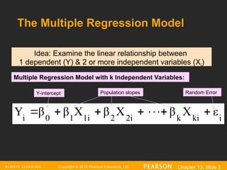
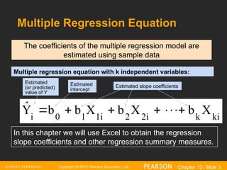
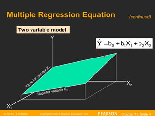
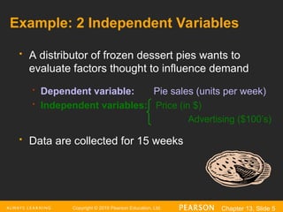
Copyright © 2016 Pearson Education, Ltd. Chapter 13, Slide 1
Introduction to Multiple
Regression
Chapter 13
Copyright © 2016 Pearson Education, Ltd. Chapter 13, Slide 2
i
ki
k
2i
2
1i
1
0
i
ε
X
β
X
β
X
β
β
Y 








The Multiple Regression Model
Idea: Examine the linear relationship between
1 dependent (Y) & 2 or more independent variables (Xi)
Multiple Regression Model with k Independent Variables:
Y-intercept Population slopes Random Error
Copyright © 2016 Pearson Education, Ltd. Chapter 13, Slide 3
ki
k
2i
2
1i
1
0
i
X
b
X
b
X
b
b
Y 







ˆ
Multiple Regression Equation
The coefficients of the multiple regression model are
estimated using sample data
Estimated
(or predicted)
value of Y
Estimated slope coefficients
Multiple regression equation with k independent variables:
Estimated
intercept
In this chapter we will use Excel to obtain the regression
slope coefficients and other regression summary measures.
Copyright © 2016 Pearson Education, Ltd. Chapter 13, Slide 4
Two variable model
Y
X1
X2
2
2
1
1
0 X
b
X
b
b
Ŷ 


Slope
for variable
X 1
Slope for variable X2
Multiple Regression Equation (continued)
Copyright © 2016 Pearson Education, Ltd. Chapter 13, Slide 5
Example: 2 Independent Variables
 A distributor of frozen dessert pies wants to
evaluate factors thought to influence demand
 Dependent variable: Pie sales (units per week)
 Independent variables: Price (in $)
Advertising ($100’s)
 Data are collected for 15 weeks
Copyright © 2016 Pearson Education, Ltd. Chapter 13, Slide 6
Pie Sales Example
Sales = b0 + b1 (Price)
+ b2 (Advertising)
Week
Pie
Sales
Price
($)
Advertising
($100s)
1 350 5.50 3.3
2 460 7.50 3.3
3 350 8.00 3.0
4 430 8.00 4.5
5 350 6.80 3.0
6 380 7.50 4.0
7 430 4.50 3.0
8 470 6.40 3.7
9 450 7.00 3.5
10 490 5.00 4.0
11 340 7.20 3.5
12 300 7.90 3.2
13 440 5.90 4.0
14 450 5.00 3.5
15 300 7.00 2.7
Multiple regression equation:
Copyright © 2016 Pearson Education, Ltd. Chapter 13, Slide 7
Regression Statistics
Multiple R 0.72213
R Square 0.52148
Adjusted R Square 0.44172
Standard Error 47.46341
Observations 15
ANOVA df SS MS F Significance F
Regression 2 29460.027 14730.013 6.53861 0.01201
Residual 12 27033.306 2252.776
Total 14 56493.333
Coefficients Standard Error t Stat P-value Lower 95% Upper 95%
Intercept 306.52619 114.25389 2.68285 0.01993 57.58835 555.46404
Price -24.97509 10.83213 -2.30565 0.03979 -48.57626 -1.37392
Advertising 74.13096 25.96732 2.85478 0.01449 17.55303 130.70888
Excel Multiple Regression Output
ertising)
74.131(Adv
ce)
24.975(Pri
-
306.526
Sales 

Copyright © 2016 Pearson Education, Ltd. Chapter 13, Slide 8
The Multiple Regression Equation
ertising)
74.131(Adv
ce)
24.975(Pri
-
306.526
Sales 

b1 = -24.975: sales
will decrease, on
average, by 24.975
pies per week for
each $1 increase in
selling price, net of
the effects of
changes due to
advertising
b2 = 74.131: sales will
increase, on average,
by 74.131 pies per
week for each $100
increase in
advertising, net of the
effects of changes
due to price
where
Sales is in number of pies per week
Price is in $
Advertising is in $100’s.
Copyright © 2016 Pearson Education, Ltd. Chapter 13, Slide 9
Using The Equation to Make Predictions
Predict sales for a week in which the selling
price is $5.50 and advertising is $350:
Predicted sales
is 428.62 pies
428.62
(3.5)
74.131
(5.50)
24.975
-
306.526
ertising)
74.131(Adv
ce)
24.975(Pri
-
306.526
Sales





Note that Advertising is
in $100s, so $350 means
that X2 = 3.5
Copyright © 2016 Pearson Education, Ltd. Chapter 13, Slide 10
The Coefficient of Multiple
Determination, r2
 Reports the proportion of total variation in Y
explained by all X variables taken together
squares
of
sum
total
squares
of
sum
regression
SST
SSR
r 

2
Copyright © 2016 Pearson Education, Ltd. Chapter 13, Slide 11
Regression Statistics
Multiple R 0.72213
R Square 0.52148
Adjusted R Square 0.44172
Standard Error 47.46341
Observations 15
ANOVA df SS MS F Significance F
Regression 2 29460.027 14730.013 6.53861 0.01201
Residual 12 27033.306 2252.776
Total 14 56493.333
Coefficients Standard Error t Stat P-value Lower 95% Upper 95%
Intercept 306.52619 114.25389 2.68285 0.01993 57.58835 555.46404
Price -24.97509 10.83213 -2.30565 0.03979 -48.57626 -1.37392
Advertising 74.13096 25.96732 2.85478 0.01449 17.55303 130.70888
.52148
56493.3
29460.0
SST
SSR
r2



52.1% of the variation in pie sales
is explained by the variation in
price and advertising
Multiple Coefficient of Determination In Excel
Copyright © 2016 Pearson Education, Ltd. Chapter 13, Slide 12
Adjusted r2
 r2
never decreases when a new X variable is
added to the model

This can be a disadvantage when comparing
models
 What is the net effect of adding a new variable?

We lose a degree of freedom when a new X
variable is added

Did the new X variable add enough
explanatory power to offset the loss of one
degree of freedom?
Copyright © 2016 Pearson Education, Ltd. Chapter 13, Slide 13
Adjusted r2
 Shows the proportion of variation in Y explained by
all X variables adjusted for the number of X
variables used
(where n = sample size, k = number of independent variables)
 Penalizes excessive use of unimportant independent
variables
 Smaller than r2
 Useful in comparing among models


















1
1
)
1
(
1 2
2
k
n
n
r
radj
(continued)
Copyright © 2016 Pearson Education, Ltd. Chapter 13, Slide 14
Regression Statistics
Multiple R 0.72213
R Square 0.52148
Adjusted R Square 0.44172
Standard Error 47.46341
Observations 15
ANOVA df SS MS F Significance F
Regression 2 29460.027 14730.013 6.53861 0.01201
Residual 12 27033.306 2252.776
Total 14 56493.333
Coefficients Standard Error t Stat P-value Lower 95% Upper 95%
Intercept 306.52619 114.25389 2.68285 0.01993 57.58835 555.46404
Price -24.97509 10.83213 -2.30565 0.03979 -48.57626 -1.37392
Advertising 74.13096 25.96732 2.85478 0.01449 17.55303 130.70888
.44172
r2
adj 
44.2% of the variation in pie sales is
explained by the variation in price and
advertising, taking into account the sample
size and number of independent variables
Adjusted r2
in Excel
Copyright © 2016 Pearson Education, Ltd. Chapter 13, Slide 15
Is the Model Significant?
 F Test for Overall Significance of the Model
 Shows if there is a linear relationship between all of the X
variables considered together and Y
 Use F-test statistic
 Hypotheses:
H0: β1 = β2 = …
= βk = 0 (no linear relationship)
H1: at least one βi ≠ 0 (at least one independent
variable affects Y)
Copyright © 2016 Pearson Education, Ltd. Chapter 13, Slide 16
F Test for Overall Significance
 Test statistic:
where FSTAT has numerator d.f. = k and
denominator d.f. = (n – k - 1)
1




k
n
SSE
k
SSR
MSE
MSR
FSTAT
Copyright © 2016 Pearson Education, Ltd. Chapter 13, Slide 17
Regression Statistics
Multiple R 0.72213
R Square 0.52148
Adjusted R Square 0.44172
Standard Error 47.46341
Observations 15
ANOVA df SS MS F Significance F
Regression 2 29460.027 14730.013 6.53861 0.01201
Residual 12 27033.306 2252.776
Total 14 56493.333
Coefficients Standard Error t Stat P-value Lower 95% Upper 95%
Intercept 306.52619 114.25389 2.68285 0.01993 57.58835 555.46404
Price -24.97509 10.83213 -2.30565 0.03979 -48.57626 -1.37392
Advertising 74.13096 25.96732 2.85478 0.01449 17.55303 130.70888
F Test for Overall Significance In Excel
With 2 and 12 degrees
of freedom
P-value for
the F Test
6.5386
2252.8
14730.0
MSE
MSR
FSTAT 


(continued)
Copyright © 2016 Pearson Education, Ltd. Chapter 13, Slide 18
F Test for Overall Significance
H0: β1 = β2 = 0
H1: β1 and β2 not both zero
 = .05
df1= 2 df2 = 12
Test Statistic:
Decision:
Conclusion:
Since FSTAT test statistic is
in the rejection region (p-
value < .05), reject H0
There is evidence that at least one
independent variable affects Y
0
 = .05
F0.05 = 3.885
Reject H0
Do not
reject H0
6.5386
FSTAT 

MSE
MSR
Critical
Value:
F0.05 = 3.885
F
(continued)
Copyright © 2016 Pearson Education, Ltd. Chapter 13, Slide 19
Multiple Regression Assumptions
Assumptions:
 The errors are normally distributed
 Errors have a constant variance
 The model errors are independent
ei = (Yi – Yi)
<
Errors (residuals) from the regression model:
Copyright © 2016 Pearson Education, Ltd. Chapter 13, Slide 20
Residual Plots Used in Multiple Regression
 These residual plots are used in multiple
regression:
 Residuals vs. Yi
 Residuals vs. X1i
 Residuals vs. X2i
 Residuals vs. time (if time series data)
<
Use the residual plots to check for
violations of regression assumptions
Copyright © 2016 Pearson Education, Ltd. Chapter 13, Slide 21
Are Individual Variables Significant?
 Use t tests of individual variable slopes
 Shows if there is a linear relationship between
the variable Xj and Y holding constant the
effects of other X variables
 Hypotheses:
 H0: βj = 0 (no linear relationship)
 H1: βj ≠ 0 (linear relationship does exist
between Xj and Y)
Copyright © 2016 Pearson Education, Ltd. Chapter 13, Slide 22
Are Individual Variables Significant?
H0: βj = 0 (no linear relationship between Xj and Y)
H1: βj ≠ 0 (linear relationship does exist
between Xj and Y)
Test Statistic:
(df = n – k – 1)
j
b
j
STAT
S
b
t
0


(continued)
Copyright © 2016 Pearson Education, Ltd. Chapter 13, Slide 23
Regression Statistics
Multiple R 0.72213
R Square 0.52148
Adjusted R Square 0.44172
Standard Error 47.46341
Observations 15
ANOVA df SS MS F Significance F
Regression 2 29460.027 14730.013 6.53861 0.01201
Residual 12 27033.306 2252.776
Total 14 56493.333
Coefficients Standard Error t Stat P-value Lower 95% Upper 95%
Intercept 306.52619 114.25389 2.68285 0.01993 57.58835 555.46404
Price -24.97509 10.83213 -2.30565 0.03979 -48.57626 -1.37392
Advertising 74.13096 25.96732 2.85478 0.01449 17.55303 130.70888
t Stat for Price is tSTAT = -2.306, with
p-value .0398
t Stat for Advertising is tSTAT = 2.855,
with p-value .0145
Are Individual Variables
Significant? Excel Output (continued)
Copyright © 2016 Pearson Education, Ltd. Chapter 13, Slide 24
d.f. = 15-2-1 = 12
 = .05
t/2 = 2.1788
Inferences about the Slope:
t Test Example
H0: βj = 0
H1: βj  0
The test statistic for each variable falls
in the rejection region (p-values < .05)
There is evidence that both
Price and Advertising affect
pie sales at  = .05
From the Excel output:
Reject H0 for each variable
Decision:
Conclusion:
Reject H0
Reject H0
/2=.025
-tα/2
Do not reject H0
0
tα/2
/2=.025
-2.1788 2.1788
For Price tSTAT = -2.306, with p-value .0398
For Advertising tSTAT = 2.855, with p-value .0145
Copyright © 2016 Pearson Education, Ltd. Chapter 13, Slide 25
Confidence Interval Estimate for the Slope
Confidence interval for the population slope βj
Example: Form a 95% confidence interval for the effect of changes in
price (X1) on pie sales:
-24.975 ± (2.1788)(10.832)
So the interval is (-48.576 , -1.374)
(This interval does not contain zero, so price has a significant effect on sales)
j
b
j S
t
b 2
/
α

Coefficients Standard Error
Intercept 306.52619 114.25389
Price -24.97509 10.83213
Advertising 74.13096 25.96732
where t has
(n – k – 1) d.f.
Here, t has
(15 – 2 – 1) = 12 d.f.
Copyright © 2016 Pearson Education, Ltd. Chapter 13, Slide 26
Confidence Interval Estimate for the Slope
Confidence interval for the population slope βj
Example: Excel output also reports these interval endpoints:
Weekly sales are estimated to be reduced by between 1.37 to
48.58 pies for each increase of $1 in the selling price, holding the
effect of advertising constant
Coefficients Standard Error … Lower 95% Upper 95%
Intercept 306.52619 114.25389 … 57.58835 555.46404
Price -24.97509 10.83213 … -48.57626 -1.37392
Advertising 74.13096 25.96732 … 17.55303 130.70888
(continued)
Copyright © 2016 Pearson Education, Ltd. Chapter 13, Slide 27
Using Dummy Variables
 A dummy variable is a categorical independent
variable with two levels:
 yes or no, on or off, male or female
 coded as 0 or 1
 Assumes the slopes associated with numerical
independent variables do not change with the
value for the categorical variable
 If more than two levels, the number of dummy
variables needed is (number of levels - 1)
Copyright © 2016 Pearson Education, Ltd. Chapter 13, Slide 28
Dummy-Variable Example
(with 2 Levels)
Let:
Y = pie sales
X1 = price
X2 = holiday (X2 = 1 if a holiday occurred during the week)
(X2 = 0 if there was no holiday that week)
2
1
0 X
b
X
b
b
Ŷ 2
1



Copyright © 2016 Pearson Education, Ltd. Chapter 13, Slide 29
Same
slope
Dummy-Variable Example
(with 2 Levels)
X1 (Price)
Y (sales)
b0 + b2
b0
1
0
1
0
1
2
0
1
0
X
b
b
(0)
b
X
b
b
Ŷ
X
b
)
b
(b
(1)
b
X
b
b
Ŷ
1
2
1
1
2
1










 Holiday
No Holiday
Different
intercept
Holiday (X2 = 1)
No Holiday (X2 = 0)
If H0: β2 = 0 is
rejected, then
“Holiday” has a
significant effect
on pie sales
DCOVA
(continued)
Copyright © 2016 Pearson Education, Ltd. Chapter 13, Slide 30
Sales: number of pies sold per week
Price: pie price in $
Holiday:
Interpreting the Dummy Variable
Coefficient (with 2 Levels)
Example:
1 If a holiday occurred during the week
0 If no holiday occurred
b2 = 15: on average, sales were 15 pies greater in
weeks with a holiday than in weeks without a
holiday, given the same price
)
15(Holiday
30(Price)
-
300
Sales 

Copyright © 2016 Pearson Education, Ltd. Chapter 13, Slide 31
Interaction Between Independent Variables
 Hypothesizes interaction between pairs of X
variables
 Response to one X variable may vary at different
levels of another X variable
 Contains two-way cross product terms

)
X
(X
b
X
b
X
b
b
X
b
X
b
X
b
b
Ŷ
2
1
3
2
2
1
1
0
3
3
2
2
1
1
0








Copyright © 2016 Pearson Education, Ltd. Chapter 13, Slide 32
Effect of Interaction
 Given:
 Without interaction term, effect of X1 on Y is
measured by β1
 With interaction term, effect of X1 on Y is
measured by β1 + β3 X2
 Effect changes as X2 changes
ε
X
X
β
X
β
X
β
β
Y 2
1
3
2
2
1
1
0 




Copyright © 2016 Pearson Education, Ltd. Chapter 13, Slide 33
X2 = 1:
Y = 1 + 2X1 + 3(1) + 4X1(1) = 4 + 6X1
X2 = 0:
Y = 1 + 2X1 + 3(0) + 4X1(0) = 1 + 2X1
Interaction Example
Slopes are different if the effect of X1 on Y depends on X2 value
X1
4
4
8
8
12
12
0
0
0
0 1
1
0.5
0.5 1.5
1.5
Y
= 1 + 2X1 + 3X2 + 4X1X2
Suppose X2 is a dummy variable and the estimated
regression equation is Ŷ
Copyright © 2016 Pearson Education, Ltd. Chapter 13, Slide 34
Chapter Summary
In this chapter we discussed:
 How to develop a multiple regression model
 How to interpret the regression coefficients
 How to determine which independent variables to
include in the regression model
 How to use categorical independent variables in a
regression model

ch13 multiple regression ppt: introduction to multiple regression

  • 1.
    Copyright © 2016Pearson Education, Ltd. Chapter 13, Slide 1 Introduction to Multiple Regression Chapter 13
  • 2.
    Copyright © 2016Pearson Education, Ltd. Chapter 13, Slide 2 i ki k 2i 2 1i 1 0 i ε X β X β X β β Y          The Multiple Regression Model Idea: Examine the linear relationship between 1 dependent (Y) & 2 or more independent variables (Xi) Multiple Regression Model with k Independent Variables: Y-intercept Population slopes Random Error
  • 3.
    Copyright © 2016Pearson Education, Ltd. Chapter 13, Slide 3 ki k 2i 2 1i 1 0 i X b X b X b b Y         ˆ Multiple Regression Equation The coefficients of the multiple regression model are estimated using sample data Estimated (or predicted) value of Y Estimated slope coefficients Multiple regression equation with k independent variables: Estimated intercept In this chapter we will use Excel to obtain the regression slope coefficients and other regression summary measures.
  • 4.
    Copyright © 2016Pearson Education, Ltd. Chapter 13, Slide 4 Two variable model Y X1 X2 2 2 1 1 0 X b X b b Ŷ    Slope for variable X 1 Slope for variable X2 Multiple Regression Equation (continued)
  • 5.
    Copyright © 2016Pearson Education, Ltd. Chapter 13, Slide 5 Example: 2 Independent Variables  A distributor of frozen dessert pies wants to evaluate factors thought to influence demand  Dependent variable: Pie sales (units per week)  Independent variables: Price (in $) Advertising ($100’s)  Data are collected for 15 weeks
  • 6.
    Copyright © 2016Pearson Education, Ltd. Chapter 13, Slide 6 Pie Sales Example Sales = b0 + b1 (Price) + b2 (Advertising) Week Pie Sales Price ($) Advertising ($100s) 1 350 5.50 3.3 2 460 7.50 3.3 3 350 8.00 3.0 4 430 8.00 4.5 5 350 6.80 3.0 6 380 7.50 4.0 7 430 4.50 3.0 8 470 6.40 3.7 9 450 7.00 3.5 10 490 5.00 4.0 11 340 7.20 3.5 12 300 7.90 3.2 13 440 5.90 4.0 14 450 5.00 3.5 15 300 7.00 2.7 Multiple regression equation:
  • 7.
    Copyright © 2016Pearson Education, Ltd. Chapter 13, Slide 7 Regression Statistics Multiple R 0.72213 R Square 0.52148 Adjusted R Square 0.44172 Standard Error 47.46341 Observations 15 ANOVA df SS MS F Significance F Regression 2 29460.027 14730.013 6.53861 0.01201 Residual 12 27033.306 2252.776 Total 14 56493.333 Coefficients Standard Error t Stat P-value Lower 95% Upper 95% Intercept 306.52619 114.25389 2.68285 0.01993 57.58835 555.46404 Price -24.97509 10.83213 -2.30565 0.03979 -48.57626 -1.37392 Advertising 74.13096 25.96732 2.85478 0.01449 17.55303 130.70888 Excel Multiple Regression Output ertising) 74.131(Adv ce) 24.975(Pri - 306.526 Sales  
  • 8.
    Copyright © 2016Pearson Education, Ltd. Chapter 13, Slide 8 The Multiple Regression Equation ertising) 74.131(Adv ce) 24.975(Pri - 306.526 Sales   b1 = -24.975: sales will decrease, on average, by 24.975 pies per week for each $1 increase in selling price, net of the effects of changes due to advertising b2 = 74.131: sales will increase, on average, by 74.131 pies per week for each $100 increase in advertising, net of the effects of changes due to price where Sales is in number of pies per week Price is in $ Advertising is in $100’s.
  • 9.
    Copyright © 2016Pearson Education, Ltd. Chapter 13, Slide 9 Using The Equation to Make Predictions Predict sales for a week in which the selling price is $5.50 and advertising is $350: Predicted sales is 428.62 pies 428.62 (3.5) 74.131 (5.50) 24.975 - 306.526 ertising) 74.131(Adv ce) 24.975(Pri - 306.526 Sales      Note that Advertising is in $100s, so $350 means that X2 = 3.5
  • 10.
    Copyright © 2016Pearson Education, Ltd. Chapter 13, Slide 10 The Coefficient of Multiple Determination, r2  Reports the proportion of total variation in Y explained by all X variables taken together squares of sum total squares of sum regression SST SSR r   2
  • 11.
    Copyright © 2016Pearson Education, Ltd. Chapter 13, Slide 11 Regression Statistics Multiple R 0.72213 R Square 0.52148 Adjusted R Square 0.44172 Standard Error 47.46341 Observations 15 ANOVA df SS MS F Significance F Regression 2 29460.027 14730.013 6.53861 0.01201 Residual 12 27033.306 2252.776 Total 14 56493.333 Coefficients Standard Error t Stat P-value Lower 95% Upper 95% Intercept 306.52619 114.25389 2.68285 0.01993 57.58835 555.46404 Price -24.97509 10.83213 -2.30565 0.03979 -48.57626 -1.37392 Advertising 74.13096 25.96732 2.85478 0.01449 17.55303 130.70888 .52148 56493.3 29460.0 SST SSR r2    52.1% of the variation in pie sales is explained by the variation in price and advertising Multiple Coefficient of Determination In Excel
  • 12.
    Copyright © 2016Pearson Education, Ltd. Chapter 13, Slide 12 Adjusted r2  r2 never decreases when a new X variable is added to the model  This can be a disadvantage when comparing models  What is the net effect of adding a new variable?  We lose a degree of freedom when a new X variable is added  Did the new X variable add enough explanatory power to offset the loss of one degree of freedom?
  • 13.
    Copyright © 2016Pearson Education, Ltd. Chapter 13, Slide 13 Adjusted r2  Shows the proportion of variation in Y explained by all X variables adjusted for the number of X variables used (where n = sample size, k = number of independent variables)  Penalizes excessive use of unimportant independent variables  Smaller than r2  Useful in comparing among models                   1 1 ) 1 ( 1 2 2 k n n r radj (continued)
  • 14.
    Copyright © 2016Pearson Education, Ltd. Chapter 13, Slide 14 Regression Statistics Multiple R 0.72213 R Square 0.52148 Adjusted R Square 0.44172 Standard Error 47.46341 Observations 15 ANOVA df SS MS F Significance F Regression 2 29460.027 14730.013 6.53861 0.01201 Residual 12 27033.306 2252.776 Total 14 56493.333 Coefficients Standard Error t Stat P-value Lower 95% Upper 95% Intercept 306.52619 114.25389 2.68285 0.01993 57.58835 555.46404 Price -24.97509 10.83213 -2.30565 0.03979 -48.57626 -1.37392 Advertising 74.13096 25.96732 2.85478 0.01449 17.55303 130.70888 .44172 r2 adj  44.2% of the variation in pie sales is explained by the variation in price and advertising, taking into account the sample size and number of independent variables Adjusted r2 in Excel
  • 15.
    Copyright © 2016Pearson Education, Ltd. Chapter 13, Slide 15 Is the Model Significant?  F Test for Overall Significance of the Model  Shows if there is a linear relationship between all of the X variables considered together and Y  Use F-test statistic  Hypotheses: H0: β1 = β2 = … = βk = 0 (no linear relationship) H1: at least one βi ≠ 0 (at least one independent variable affects Y)
  • 16.
    Copyright © 2016Pearson Education, Ltd. Chapter 13, Slide 16 F Test for Overall Significance  Test statistic: where FSTAT has numerator d.f. = k and denominator d.f. = (n – k - 1) 1     k n SSE k SSR MSE MSR FSTAT
  • 17.
    Copyright © 2016Pearson Education, Ltd. Chapter 13, Slide 17 Regression Statistics Multiple R 0.72213 R Square 0.52148 Adjusted R Square 0.44172 Standard Error 47.46341 Observations 15 ANOVA df SS MS F Significance F Regression 2 29460.027 14730.013 6.53861 0.01201 Residual 12 27033.306 2252.776 Total 14 56493.333 Coefficients Standard Error t Stat P-value Lower 95% Upper 95% Intercept 306.52619 114.25389 2.68285 0.01993 57.58835 555.46404 Price -24.97509 10.83213 -2.30565 0.03979 -48.57626 -1.37392 Advertising 74.13096 25.96732 2.85478 0.01449 17.55303 130.70888 F Test for Overall Significance In Excel With 2 and 12 degrees of freedom P-value for the F Test 6.5386 2252.8 14730.0 MSE MSR FSTAT    (continued)
  • 18.
    Copyright © 2016Pearson Education, Ltd. Chapter 13, Slide 18 F Test for Overall Significance H0: β1 = β2 = 0 H1: β1 and β2 not both zero  = .05 df1= 2 df2 = 12 Test Statistic: Decision: Conclusion: Since FSTAT test statistic is in the rejection region (p- value < .05), reject H0 There is evidence that at least one independent variable affects Y 0  = .05 F0.05 = 3.885 Reject H0 Do not reject H0 6.5386 FSTAT   MSE MSR Critical Value: F0.05 = 3.885 F (continued)
  • 19.
    Copyright © 2016Pearson Education, Ltd. Chapter 13, Slide 19 Multiple Regression Assumptions Assumptions:  The errors are normally distributed  Errors have a constant variance  The model errors are independent ei = (Yi – Yi) < Errors (residuals) from the regression model:
  • 20.
    Copyright © 2016Pearson Education, Ltd. Chapter 13, Slide 20 Residual Plots Used in Multiple Regression  These residual plots are used in multiple regression:  Residuals vs. Yi  Residuals vs. X1i  Residuals vs. X2i  Residuals vs. time (if time series data) < Use the residual plots to check for violations of regression assumptions
  • 21.
    Copyright © 2016Pearson Education, Ltd. Chapter 13, Slide 21 Are Individual Variables Significant?  Use t tests of individual variable slopes  Shows if there is a linear relationship between the variable Xj and Y holding constant the effects of other X variables  Hypotheses:  H0: βj = 0 (no linear relationship)  H1: βj ≠ 0 (linear relationship does exist between Xj and Y)
  • 22.
    Copyright © 2016Pearson Education, Ltd. Chapter 13, Slide 22 Are Individual Variables Significant? H0: βj = 0 (no linear relationship between Xj and Y) H1: βj ≠ 0 (linear relationship does exist between Xj and Y) Test Statistic: (df = n – k – 1) j b j STAT S b t 0   (continued)
  • 23.
    Copyright © 2016Pearson Education, Ltd. Chapter 13, Slide 23 Regression Statistics Multiple R 0.72213 R Square 0.52148 Adjusted R Square 0.44172 Standard Error 47.46341 Observations 15 ANOVA df SS MS F Significance F Regression 2 29460.027 14730.013 6.53861 0.01201 Residual 12 27033.306 2252.776 Total 14 56493.333 Coefficients Standard Error t Stat P-value Lower 95% Upper 95% Intercept 306.52619 114.25389 2.68285 0.01993 57.58835 555.46404 Price -24.97509 10.83213 -2.30565 0.03979 -48.57626 -1.37392 Advertising 74.13096 25.96732 2.85478 0.01449 17.55303 130.70888 t Stat for Price is tSTAT = -2.306, with p-value .0398 t Stat for Advertising is tSTAT = 2.855, with p-value .0145 Are Individual Variables Significant? Excel Output (continued)
  • 24.
    Copyright © 2016Pearson Education, Ltd. Chapter 13, Slide 24 d.f. = 15-2-1 = 12  = .05 t/2 = 2.1788 Inferences about the Slope: t Test Example H0: βj = 0 H1: βj  0 The test statistic for each variable falls in the rejection region (p-values < .05) There is evidence that both Price and Advertising affect pie sales at  = .05 From the Excel output: Reject H0 for each variable Decision: Conclusion: Reject H0 Reject H0 /2=.025 -tα/2 Do not reject H0 0 tα/2 /2=.025 -2.1788 2.1788 For Price tSTAT = -2.306, with p-value .0398 For Advertising tSTAT = 2.855, with p-value .0145
  • 25.
    Copyright © 2016Pearson Education, Ltd. Chapter 13, Slide 25 Confidence Interval Estimate for the Slope Confidence interval for the population slope βj Example: Form a 95% confidence interval for the effect of changes in price (X1) on pie sales: -24.975 ± (2.1788)(10.832) So the interval is (-48.576 , -1.374) (This interval does not contain zero, so price has a significant effect on sales) j b j S t b 2 / α  Coefficients Standard Error Intercept 306.52619 114.25389 Price -24.97509 10.83213 Advertising 74.13096 25.96732 where t has (n – k – 1) d.f. Here, t has (15 – 2 – 1) = 12 d.f.
  • 26.
    Copyright © 2016Pearson Education, Ltd. Chapter 13, Slide 26 Confidence Interval Estimate for the Slope Confidence interval for the population slope βj Example: Excel output also reports these interval endpoints: Weekly sales are estimated to be reduced by between 1.37 to 48.58 pies for each increase of $1 in the selling price, holding the effect of advertising constant Coefficients Standard Error … Lower 95% Upper 95% Intercept 306.52619 114.25389 … 57.58835 555.46404 Price -24.97509 10.83213 … -48.57626 -1.37392 Advertising 74.13096 25.96732 … 17.55303 130.70888 (continued)
  • 27.
    Copyright © 2016Pearson Education, Ltd. Chapter 13, Slide 27 Using Dummy Variables  A dummy variable is a categorical independent variable with two levels:  yes or no, on or off, male or female  coded as 0 or 1  Assumes the slopes associated with numerical independent variables do not change with the value for the categorical variable  If more than two levels, the number of dummy variables needed is (number of levels - 1)
  • 28.
    Copyright © 2016Pearson Education, Ltd. Chapter 13, Slide 28 Dummy-Variable Example (with 2 Levels) Let: Y = pie sales X1 = price X2 = holiday (X2 = 1 if a holiday occurred during the week) (X2 = 0 if there was no holiday that week) 2 1 0 X b X b b Ŷ 2 1   
  • 29.
    Copyright © 2016Pearson Education, Ltd. Chapter 13, Slide 29 Same slope Dummy-Variable Example (with 2 Levels) X1 (Price) Y (sales) b0 + b2 b0 1 0 1 0 1 2 0 1 0 X b b (0) b X b b Ŷ X b ) b (b (1) b X b b Ŷ 1 2 1 1 2 1            Holiday No Holiday Different intercept Holiday (X2 = 1) No Holiday (X2 = 0) If H0: β2 = 0 is rejected, then “Holiday” has a significant effect on pie sales DCOVA (continued)
  • 30.
    Copyright © 2016Pearson Education, Ltd. Chapter 13, Slide 30 Sales: number of pies sold per week Price: pie price in $ Holiday: Interpreting the Dummy Variable Coefficient (with 2 Levels) Example: 1 If a holiday occurred during the week 0 If no holiday occurred b2 = 15: on average, sales were 15 pies greater in weeks with a holiday than in weeks without a holiday, given the same price ) 15(Holiday 30(Price) - 300 Sales  
  • 31.
    Copyright © 2016Pearson Education, Ltd. Chapter 13, Slide 31 Interaction Between Independent Variables  Hypothesizes interaction between pairs of X variables  Response to one X variable may vary at different levels of another X variable  Contains two-way cross product terms  ) X (X b X b X b b X b X b X b b Ŷ 2 1 3 2 2 1 1 0 3 3 2 2 1 1 0        
  • 32.
    Copyright © 2016Pearson Education, Ltd. Chapter 13, Slide 32 Effect of Interaction  Given:  Without interaction term, effect of X1 on Y is measured by β1  With interaction term, effect of X1 on Y is measured by β1 + β3 X2  Effect changes as X2 changes ε X X β X β X β β Y 2 1 3 2 2 1 1 0     
  • 33.
    Copyright © 2016Pearson Education, Ltd. Chapter 13, Slide 33 X2 = 1: Y = 1 + 2X1 + 3(1) + 4X1(1) = 4 + 6X1 X2 = 0: Y = 1 + 2X1 + 3(0) + 4X1(0) = 1 + 2X1 Interaction Example Slopes are different if the effect of X1 on Y depends on X2 value X1 4 4 8 8 12 12 0 0 0 0 1 1 0.5 0.5 1.5 1.5 Y = 1 + 2X1 + 3X2 + 4X1X2 Suppose X2 is a dummy variable and the estimated regression equation is Ŷ
  • 34.
    Copyright © 2016Pearson Education, Ltd. Chapter 13, Slide 34 Chapter Summary In this chapter we discussed:  How to develop a multiple regression model  How to interpret the regression coefficients  How to determine which independent variables to include in the regression model  How to use categorical independent variables in a regression model