Downloaded 475 times
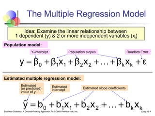
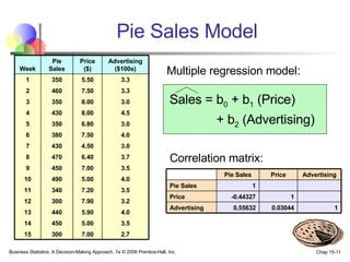

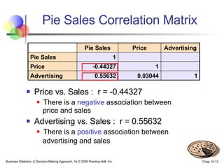
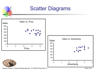
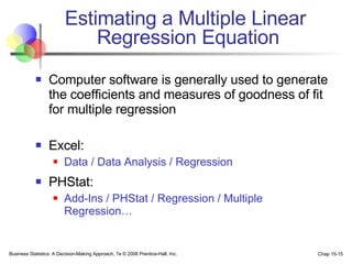
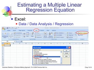

This document covers multiple regression analysis, emphasizing model building, significance testing of independent variables, and interpreting results in business contexts. It details the development of regression models, the evaluation of coefficients, and methods to assess model fit while addressing issues like multicollinearity and the use of dummy variables. Practical examples illustrate the process of predicting outcomes and determining the relationships between variables such as price and advertising on pie sales.


