Forecasting
• Forecasting isthe process of making predictions based on past and
present data. Basically, it is a decision-making tool that helps
businesses cope with the impact of the future's uncertainty by
examining historical data and trends.
• Short Term Forecasting
• Long Term Forecasting
3.
Benefits of Forecasting
•Better utilization of resources
• Formulating business plans
• Enhance the quality of management
• Helps in establishing new business model.
• Helps in making the best managerial decisions
4.
Predictive Analytics
• Predictiveanalytics is the process of using data to forecast future
outcomes. The process uses data analysis, machine learning,
artificial intelligence, and statistical models to find patterns that
might predict future behavior.
5.
Process of PredictiveAnalytics
• Defining the project
• Collecting the data
• Analyzing the data
• Deploying the statistics
6.
Regression
• A regressionis a statistical technique that relates a dependent
variable to one or more independent (explanatory) variables. A
regression model is able to show whether changes observed in
the dependent variable are associated with changes in one or
more of the explanatory variables.
7.
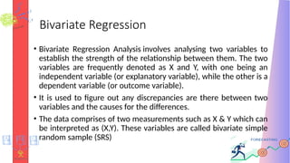
Bivariate Regression
• BivariateRegression Analysis involves analysing two variables to
establish the strength of the relationship between them. The two
variables are frequently denoted as X and Y, with one being an
independent variable (or explanatory variable), while the other is a
dependent variable (or outcome variable).
• It is used to figure out any discrepancies are there between two
variables and the causes for the differences.
• The data comprises of two measurements such as X & Y which can
be interpreted as (X,Y). These variables are called bivariate simple
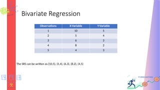
random sample (SRS)
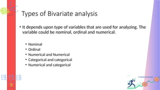
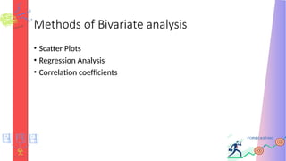
Types of Bivariateanalysis
• It depends upon type of variables that are used for analyzing. The
variable could be nominal, ordinal and numerical.
• Nominal
• Ordinal
• Numerical and Numerical
• Categorical and categorical
• Numerical and categorical
10.
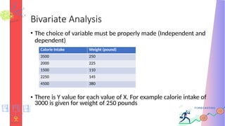
Bivariate Analysis
• Thechoice of variable must be properly made (Independent and
dependent)
Calorie Intake Weight (pound)
3500 250
2000 225
1500 110
2250 145
4500 380
• There is Y value for each value of X. For example calorie intake of
3000 is given for weight of 250 pounds
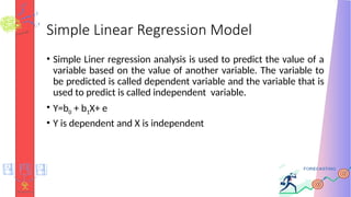
Simple Linear RegressionModel
• Simple Liner regression analysis is used to predict the value of a
variable based on the value of another variable. The variable to
be predicted is called dependent variable and the variable that is
used to predict is called independent variable.
• Y=b0 + b1X+ e
• Y is dependent and X is independent
13.
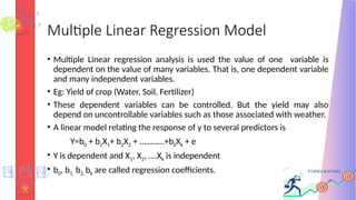
Multiple Linear RegressionModel
• Multiple Linear regression analysis is used the value of one variable is
dependent on the value of many variables. That is, one dependent variable
and many independent variables.
• Eg: Yield of crop (Water, Soil, Fertilizer)
• These dependent variables can be controlled. But the yield may also
depend on uncontrollable variables such as those associated with weather.
• A linear model relating the response of y to several predictors is
Y=b0 + b1X1+ b2X2 + …………+bkXk + e
• Y is dependent and X1, X2, ….Xk is independent
• b0, b1, b2, bk are called regression coefficients.
14.
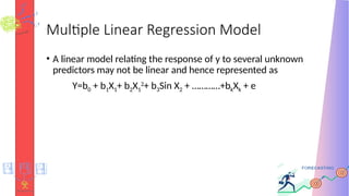
Multiple Linear RegressionModel
• A linear model relating the response of y to several unknown
predictors may not be linear and hence represented as
Y=b0 + b1X1+ b2X1
2
+ b3Sin X2 + …………+bkXk + e
15.
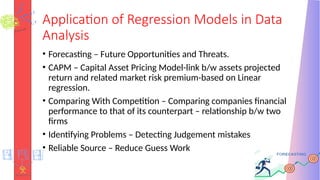
Application of RegressionModels in Data
Analysis
• Forecasting – Future Opportunities and Threats.
• CAPM – Capital Asset Pricing Model-link b/w assets projected
return and related market risk premium-based on Linear
regression.
• Comparing With Competition – Comparing companies financial
performance to that of its counterpart – relationship b/w two
firms
• Identifying Problems – Detecting Judgement mistakes
• Reliable Source – Reduce Guess Work
16.
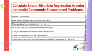
Calculate Linear BivariateRegression in order
to model Commonly Encountered Problems.
Linear – Fitting a Straight line through the given points
Bivariate – Two Variables
The expression of linear regression is y = b0 + b1x + e
e is an error term and is included to make both sides equal.
b0 & b1 are the regression coefficients need to be estimated.
b0 is the constant in the model also called intercept.
b1 is the slope of the model and is represented as change in ‘y’ by a change of 1 unit in ‘x’
17.
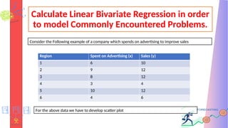
Calculate Linear BivariateRegression in order
to model Commonly Encountered Problems.
For the above data we have to develop scatter plot
Consider the Following example of a company which spends on advertising to improve sales
Region Spent on Advertising (x) Sales (y)
1 6 10
2 9 12
3 8 12
4 3 4
5 10 12
6 4 6
18.
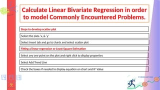
Calculate Linear BivariateRegression in order
to model Commonly Encountered Problems.
Select the data ‘x, & ‘y’
Steps to develop scatter plot
Select insert tab and go to charts and select scatter plot
Fitting a linear regression or Least Square Estimation
Select any one point on the plot and right click to display properties
Select Add Trend Line
Check the boxes if needed to display equation on chart and R2
Value
19.
Calculate Linear BivariateRegression in order
to model Commonly Encountered Problems.
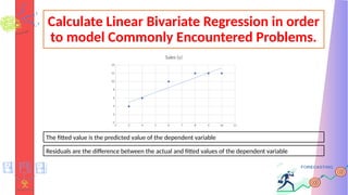
The fitted value is the predicted value of the dependent variable
2 3 4 5 6 7 8 9 10 11
0
2
4
6
8
10
12
14
Sales (y)
Residuals are the difference between the actual and fitted values of the dependent variable
20.
Calculate Linear BivariateRegression in order
to model Commonly Encountered Problems.
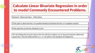
Residual = Observed Value – Fitted Value
If the point is above the line, It is positive Residual and below the line, it is negative residual.
If the point lies on the line, Residual is zero
The best fitting line for given data is the line with the smallest sum of squared residuals called least
square line. Thus the observed line is y = a + bx which is the equation of straight line.
21.
Calculate Linear BivariateRegression in order
to model Commonly Encountered Problems.
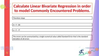
Therefore slope
A = Y - bX
e = Y – YA
The errors can be summarized by a single numerical value called Standard Error that is the standard
deviation of all errors
22.
Determine the Qualityof Fit of a Linear Model
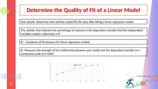
R2
– Goodness of fit measure for linear regression models
The statistic that indicates the percentage of variance in the dependent variable that the independent
variables explain collectively is R2
R2
Measures the strength of the relationship between your model and the dependent variable on a
convenient scale of 0-100%
One should determine how well the model fits the data after fitting a linear regression model.
2 3 4 5 6 7 8 9 10 11
0
2
4
6
8
10
12
14
Sales (y)
23.
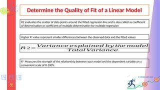
Determine the Qualityof Fit of a Linear Model
𝑅 2=
𝑉𝑎𝑟𝑖𝑎𝑛𝑐𝑒 𝑒𝑥𝑝𝑙𝑎𝑖𝑛𝑒𝑑 𝑏𝑦 h
𝑡 𝑒 𝑚𝑜𝑑𝑒𝑙
𝑇𝑜𝑡𝑎𝑙 𝑉𝑎𝑟𝑖𝑎𝑛𝑐𝑒
Higher R2
value represent smaller differences between the observed data and the fitted values
R2
Measures the strength of the relationship between your model and the dependent variable on a
convenient scale of 0-100%
R2 evaluates the scatter of data points around the fitted regression line and is also called as coefficient
of determination or coefficient of multiple determination for multiple regression
24.
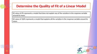
Determine the Qualityof Fit of a Linear Model
R2 value of 0% represents a model that does not explain any of the variation in the response variable
around its mean.
R2 value of 100% represents a model that explains all the variation in the response variable around its
mean.
25.
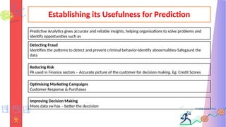
Establishing its Usefulnessfor Prediction
Predictive Analytics gives accurate and reliable insights, helping organisations to solve problems and
identify opportunities such as
Detecting Fraud
Identifies the patterns to detect and prevent criminal behavior-Identify abnormalities-Safegaurd the
data
Reducing Risk
PA used in Finance sectors – Accurate picture of the customer for decision making. Eg: Credit Scores
Optimising Marketing Campaigns
Customer Response & Purchases
Improving Decision Making
More data sw has – better the deccision
26.
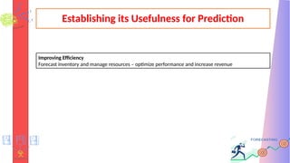
Establishing its Usefulnessfor Prediction
Improving Efficiency
Forecast inventory and manage resources – optimize performance and increase revenue
27.
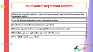
Multivariate Regression Analysis
MultivariateRegression analysis is a supervised machine learning algorithm involving multiple data
variables for analysis
It has one dependent variable and many independent variables.
Based on the number of variables, the output is predicted.
The simple regression is linear meaning straight line represents a function y of x.
The multiple regression is planar that represents extra dimensions
Y= bo + b1.x1 + b2.x2+ ……….. + bn.xn
28.
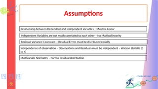
Assumptions
Independent Variables arenot much correlated to each other – No Multicollinearity
Relationship between Dependent and Independent Variables – Must be Linear
Residual Variance is constant – Residual Errors must be distributed equally
Independence of observation – Observations and Residuals must be independent – Watson Statistic (0
to 4)
Multivariate Normality – normal residual distribution
29.
Calculate Linear MultivariateRegression in order to model Commonly
Encountered Problems.
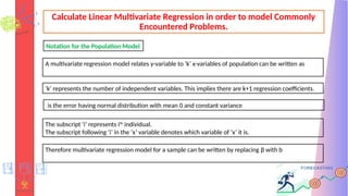
A multivariate regression model relates y-variable to ‘k’ x-variables of population can be written as
‘k’ represents the number of independent variables. This implies there are k+1 regression coefficients.
is the error having normal distribution with mean 0 and constant variance
The subscript ‘i’ represents ith
individual.
The subscript following ‘i’ in the ‘x’ variable denotes which variable of ‘x’ it is.
Therefore multivariate regression model for a sample can be written by replacing β with b
Notation for the Population Model
30.
Calculate Linear MultivariateRegression in order to model Commonly
Encountered Problems.
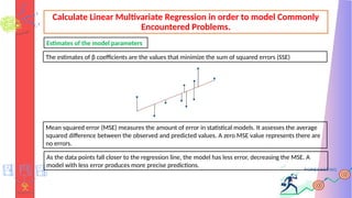
The estimates of β coefficients are the values that minimize the sum of squared errors (SSE)
Mean squared error (MSE) measures the amount of error in statistical models. It assesses the average
squared difference between the observed and predicted values. A zero MSE value represents there are
no errors.
Estimates of the model parameters
As the data points fall closer to the regression line, the model has less error, decreasing the MSE. A
model with less error produces more precise predictions.
31.
Calculate Linear MultivariateRegression in order to model Commonly
Encountered Problems.
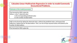
The formula for MSE is given by
Where is the ith
observed value
is the Corresponding predicted value
n is the number of observation
Estimates of the model parameters
MSE can be found by taking the observed value, subtract the predicted value, and square that
difference. Repeat that for all observations. Then, sum all of those squared values and divide by the
number of observations.
The formula for MSE is given by
32.
Calculate Linear MultivariateRegression in order to model Commonly
Encountered Problems.
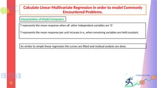
T represents the mean response when all other independent variables are ‘0’
T represents the mean response per unit increase in x1 when remaining variables are held constant.
Interpretation of Model Computers
As similar to simple linear regression the curves are fitted and residual analysis are done.
33.
Determine the Qualityof Fit of a Linear Model
𝑅 2=
𝑉𝑎𝑟𝑖𝑎𝑛𝑐𝑒 𝑒𝑥𝑝𝑙𝑎𝑖𝑛𝑒𝑑 𝑏𝑦 h
𝑡 𝑒 𝑚𝑜𝑑𝑒𝑙
𝑇𝑜𝑡𝑎𝑙 𝑉𝑎𝑟𝑖𝑎𝑛𝑐𝑒
Higher R2
value represent smaller differences between the observed data and the fitted values
R2
Measures the strength of the relationship between your model and the dependent variable on a
convenient scale of 0-100%
R2 evaluates the scatter of data points around the fitted regression line and is also called as coefficient
of determination or coefficient of multiple determination for multiple regression
34.
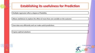
Establishing its usefulnessfor Prediction
Uses data very efficiently and can make useful predictions
Allows statistician to explore the effect of more than one variable on the outcome
It gives optimal solutions
Multiple regression offers a degree of flexibility.
35.
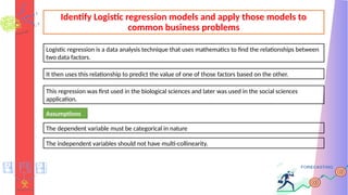
Identify Logistic regressionmodels and apply those models to
common business problems
Logistic regression is a data analysis technique that uses mathematics to find the relationships between
two data factors.
It then uses this relationship to predict the value of one of those factors based on the other.
This regression was first used in the biological sciences and later was used in the social sciences
application.
Assumptions
The dependent variable must be categorical in nature
The independent variables should not have multi-collinearity.
36.
Identify Logistic regressionmodels and apply those models to
common business problems
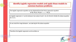
The logistic regression equation can be obtained from the linear regression equation
y= b0 + b1.x1 + b2.x2+ ……….. + bn.xn
In logistic regression ‘y’ can be between two values 0 and 1. So, for this let’s divide the above equation
by 1-y i.e,
As we need the range between , we take log for the above equation
Therefore the logistic regression can be written as
37.
Types of LogsticRegression
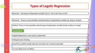
Binomial - Two types of dependent variable |(0 or 1; Yes or No; Pass or Fail)
Binomial - Three or more possible unordered types of dependent variable (cat, dogs or sheeps)
Ordinal: Three or more possible ordered types of dependent variable (Small, medium or Large)
Assumptions
Logistic Regression is very easy to understand
It Requires less Training
It performs well for simple data sets and data sets is linearly seperable
It is less likely to be overfitted.
38.
Forecasting in Time
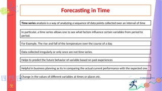
Timeseries analysis is a way of analyzing a sequence of data points collected over an interval of time
In particular, a time series allows one to see what factors influence certain variables from period to
period.
For Example, The rise and fall of the temperature over the course of a day.
Data collected irregularly or only once are not time series.
Helps to predict the future behavior of variable based on past experiences
Helpful in business planning as its in comparing the actual current performance with the expected one
Change in the values of different variables at times or places etc.
39.
Identify the componentsof time forecast in order to predict future
values from a model
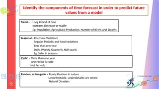
Trend – Long Period of time
Increase, Decrease or stable
Eg: Population, Agricultural Production, Number of Births and Deaths
Seasonal - Rhythmic Variations
Regular, Periodic and fixed variations
Less than one year
Daily, Weekly, Quarterly, Half yearly
Eg: Sales in seasons
Cyclic – More than one year
one Period is cycle
Not Periodic
Random or Irregular – Purely Random in nature
Uncontrollable, unpredictable are erratic
Natural Disasters
40.
Differentiate Seasonal Variationfrom trends in order to improve
prediction of future values from a model
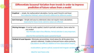
Graphical – simple, No mathematical calculation, Can be used if trend is not linear
Not subjective Method, values of trend is different for different analyst.
Semi Averages – Simple and easy to understand, does not require many calculations
Used only for linear trend, extreme values are effected
Moving Averages– It can be easily applied, Useful in periodic variations, Same value for
any analyst
Non-Periodic data is less effective, Period selection is very important,
value for first and last few years cannot be found
Method of Least Squares– Eliminates personal bias, trend values for all the given time
period is obtained, Enables to forecast future values perfectly.
Calculations are difficult, Addition of new observations require
recalculations, ignores cyclical, seasonal and irregular variations,
Ideal for near future only
41.
Differentiate Seasonal Variationfrom trends in order to improve
prediction of future values from a model
Simple Average Methods
Ratio to Trend Method
Percentage moving Average Method
Link Relative Method
42.
Calculate seasonal indicesso that seasonal variations can be
qualified in the model
Simple Average Methods
Ratio to Trend Method
Percentage moving Average Method
Link Relative Method
43.
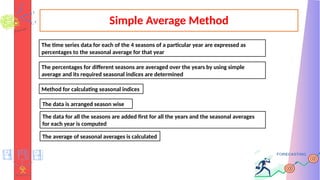
Simple Average Method
Thetime series data for each of the 4 seasons of a particular year are expressed as
percentages to the seasonal average for that year
The percentages for different seasons are averaged over the years by using simple
average and its required seasonal indices are determined
Method for calculating seasonal indices
The data is arranged season wise
The data for all the seasons are added first for all the years and the seasonal averages
for each year is computed
The average of seasonal averages is calculated
44.
Simple Average Method
Theseasonal average for each year is divided by the corresponding grand average and
the results are expressed in percentages and these are called seasonal indices
𝐺𝑟𝑎𝑛𝑑 𝐴𝑣𝑒𝑟𝑎𝑔𝑒=
𝑇𝑜𝑡𝑎𝑙 𝑜𝑓 𝑆𝑒𝑎𝑠𝑜𝑛𝑎𝑙 𝐴𝑣𝑒𝑟𝑎𝑔𝑒𝑠
4
𝑆𝑒𝑎𝑠𝑜𝑛𝑎𝑙 𝐼𝑛𝑑𝑒𝑥 =
𝑆𝑒𝑎𝑠𝑜𝑛𝑎𝑙 𝐴𝑣𝑒𝑟𝑎𝑔𝑒
𝐺𝑟𝑎𝑛𝑑 𝐴𝑣𝑒𝑟𝑎𝑔𝑒
𝑋 100
45.
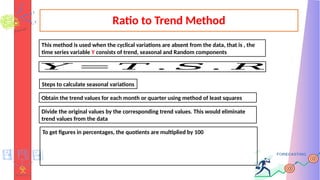
Ratio to TrendMethod
This method is used when the cyclical variations are absent from the data, that is , the
time series variable Y consists of trend, seasonal and Random components
𝑌 = 𝑇 . 𝑆 . 𝑅
Steps to calculate seasonal variations
Obtain the trend values for each month or quarter using method of least squares
Divide the original values by the corresponding trend values. This would eliminate
trend values from the data
To get figures in percentages, the quotients are multiplied by 100
46.
Percentage Moving AverageMethod
It is most commonly used method of measuring seasonal variations.
This method has all 4 components of time series
Steps to calculate seasonal variations
Compute the moving averages with period equal to the period of seasonal variations.
This will eliminate seasonal effect and minimize random component.
The original values for each quarter (or month) are divided by the respective moving
average figures and the ratio is expressed as percentage
To get figures in percentages, the quotients are multiplied by 100
47.
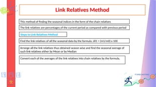
Link Relatives Method
Thismethod of finding the seasonal indices in the form of the chain relatives
The link relatives are percentages of the current period as compared with previous period
Steps to Link Relatives Method
Find the link relatives of all the seasonal data by the formula, LR1 = (m1/m0) x 100
Arrange all the link relatives thus obtained season wise and find the seasonal average of
such link relatives either by Mean or by Median
Convert each of the averages of the link relatives into chain relatives by the formula,
48.
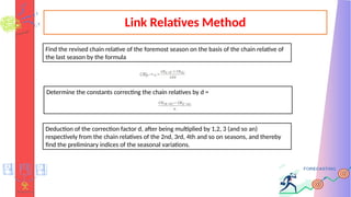
Link Relatives Method
Findthe revised chain relative of the foremost season on the basis of the chain relative of
the last season by the formula
Determine the constants correcting the chain relatives by d =
Deduction of the correction factor d, after being multiplied by 1,2, 3 (and so an)
respectively from the chain relatives of the 2nd, 3rd, 4th and so on seasons, and thereby
find the preliminary indices of the seasonal variations.
49.
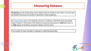
Measuring Distance
Clustering consistsof grouping certain objects that are similar to each other, it can be used
to decide if two items are similar or dissimilar in their properties.
In a Data Mining sense, the similarity measure is a distance with dimensions describing
object features. That means if the distance among two data points is small then there is
a high degree of similarity among the objects and vice versa.
The number of input variables or datasets is called dimensionality
50.
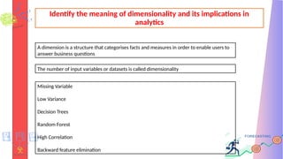
Identify the meaningof dimensionality and its implications in
analytics
A dimension is a structure that categorises facts and measures in order to enable users to
answer business questions
The number of input variables or datasets is called dimensionality
Missing Variable
Low Variance
Decision Trees
Random Forest
High Correlation
Backward feature elimination
51.
Calculate different typesof distances and identify
scenarios when each type is applicable
The different types of distances are
1. Minkowski Distance
2. Euclidean Distance
3. Manhattan Distance
4. Cosine Distance
5. Jaccard distance
6. Hamming Distance
52.
Minkowski Distance
Minkowski distanceis a distance measured between two points in
N-dimensional space.
It is widely used in the field of Machine learning, especially in the
classification of data.
Minkowski distance is used in certain algorithms like K-Nearest
Neighbors, K-Means Clustering etc.
Satisfying Conditions
- Non-Negativity: d(x,y)>=0
- Identity: d(x,y) = 0 if and only if x=y
53.
Minkowski Distance
Symmetry: d(x,y)= d(y,x)
Triangle Inequality: d(x,y) + d(y,z) = d(x,z)
Let the points be
P1: (x1,x2,………xn) & P2: (y1,y2,……yn)
The formula for minkowski is given by
54.
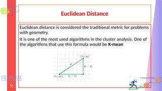
Euclidean Distance
Euclidean distanceis considered the traditional metric for problems
with geometry.
It is one of the most used algorithms in the cluster analysis. One of
the algorithms that use this formula would be K-mean
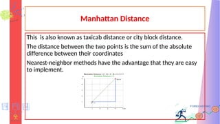
Manhattan Distance
This isalso known as taxicab distance or city block distance.
The distance between the two points is the sum of the absolute
difference between their coordinates
Nearest-neighbor methods have the advantage that they are easy
to implement.
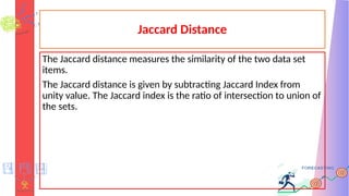
Jaccard Distance
The Jaccarddistance measures the similarity of the two data set
items.
The Jaccard distance is given by subtracting Jaccard Index from
unity value. The Jaccard index is the ratio of intersection to union of
the sets.
59.
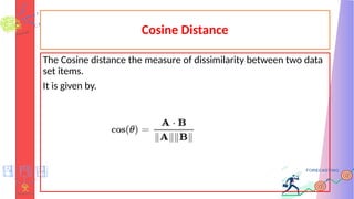
Cosine Distance
The Cosinedistance the measure of dissimilarity between two data
set items.
It is given by.
60.
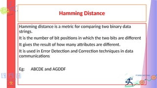
Hamming Distance
Hamming distanceis a metric for comparing two binary data
strings.
It is the number of bit positions in which the two bits are different
It gives the result of how many attributes are different.
It is used in Error Detection and Correction techniques in data
communications
Eg: ABCDE and AGDDF
61.
Unit - 2
Asubset of artificial intelligence known as machine learning
focuses primarily on the creation of algorithms that enable a
computer to independently learn from data and previous
experiences.
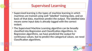
Supervised Learning
• Supervisedlearning is the types of machine learning in which
machines are trained using well "labelled" training data, and on
basis of that data, machines predict the output. The labelled data
means some input data is already tagged with the correct
output.
• The Supervised Machine Learning algorithm can be broadly
classified into Regression and Classification Algorithms. In
Regression algorithms, we have predicted the output for
continuous values, but to predict the categorical values, we need
Classification algorithms.
65.
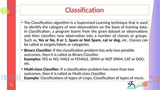
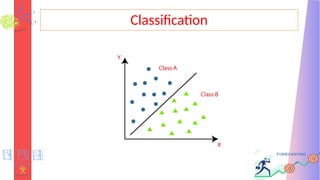
Classification
• The Classificationalgorithm is a Supervised Learning technique that is used
to identify the category of new observations on the basis of training data.
In Classification, a program learns from the given dataset or observations
and then classifies new observation into a number of classes or groups.
Such as, Yes or No, 0 or 1, Spam or Not Spam, cat or dog, etc. Classes can
be called as targets/labels or categories.
• Binary Classifier: If the classification problem has only two possible
outcomes, then it is called as Binary Classifier.
Examples: YES or NO, MALE or FEMALE, SPAM or NOT SPAM, CAT or DOG,
etc.
• Multi-class Classifier: If a classification problem has more than two
outcomes, then it is called as Multi-class Classifier.
Example: Classifications of types of crops, Classification of types of music.
66.
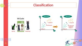
Classification
• The Classificationalgorithm is a Supervised Learning technique that is used
to identify the category of new observations on the basis of training data.
In Classification, a program learns from the given dataset or observations
and then classifies new observation into a number of classes or groups.
Such as, Yes or No, 0 or 1, Spam or Not Spam, cat or dog, etc. Classes can
be called as targets/labels or categories.
• Binary Classifier: If the classification problem has only two possible
outcomes, then it is called as Binary Classifier.
Examples: YES or NO, MALE or FEMALE, SPAM or NOT SPAM, CAT or DOG,
etc.
• Multi-class Classifier: If a classification problem has more than two
outcomes, then it is called as Multi-class Classifier.
Example: Classifications of types of crops, Classification of types of music.
KNN Algorithm
• K-NearestNeighbour is one of the simplest Machine Learning
algorithms based on Supervised Learning technique.
• K-NN algorithm assumes the similarity between the new
case/data and available cases and put the new case into the
category that is most similar to the available categories.
• K-NN algorithm stores all the available data and classifies a new
data point based on the similarity. This means when new data
appears then it can be easily classified into a well suite category
by using K- NN algorithm.
• K-NN algorithm can be used for Regression as well as for
Classification but mostly it is used for the Classification problems.
69.
KNN Algorithm
• K-NNis a non-parametric algorithm, which means it does not
make any assumption on underlying data.
• It is also called a lazy learner algorithm because it does not learn
from the training set immediately instead it stores the dataset
and at the time of classification, it performs an action on the
dataset.
• KNN algorithm at the training phase just stores the dataset and
when it gets new data, then it classifies that data into a category
that is much similar to the new data.
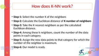
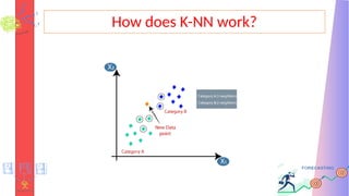
How does K-NNwork?
• Step-1: Select the number K of the neighbors
• Step-2: Calculate the Euclidean distance of K number of neighbors
• Step-3: Take the K nearest neighbors as per the calculated
Euclidean distance.
• Step-4: Among these k neighbors, count the number of the data
points in each category.
• Step-5: Assign the new data points to that category for which the
number of the neighbor is maximum.
• Step-6: Our model is ready.
Advantages of KNNAlgorithm:
• It is simple to implement.
• It is robust to the noisy training data
• It can be more effective if the training data is large.
74.
Disadvantages of KNNAlgorithm:
• Always needs to determine the value of K which may be complex
some time.
• The computation cost is high because of calculating the distance
between the data points for all the training samples.
75.
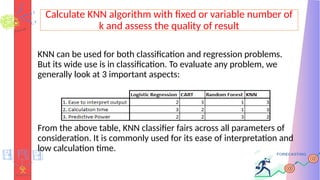
Calculate KNN algorithmwith fixed or variable number of
k and assess the quality of result
KNN can be used for both classification and regression problems.
But its wide use is in classification. To evaluate any problem, we
generally look at 3 important aspects:
From the above table, KNN classifier fairs across all parameters of
consideration. It is commonly used for its ease of interpretation and
low calculation time.
76.
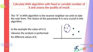
Calculate KNN algorithmwith fixed or variable number of
k and assess the quality of result
The “K” in KNN algorithm is the nearest neighbor we wish to take
the vote from. The choice of the parameter K is very crucial in this
algorithm.
In the example the value of k=3,
Likewise the analysis is performed
for different values of k.
77.
Calculate KNN algorithmwith fixed or variable number of
k and assess the quality of result
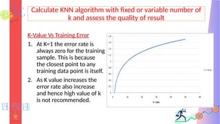
K-Value Vs Training Error
1. At K=1 the error rate is
always zero for the training
sample. This is because
the closest point to any
training data point is itself.
2. As K value increases the
error rate also increase
and hence high value of k
is not recommended.
78.
Calculate KNN algorithmwith fixed or variable number of
k and assess the quality of result
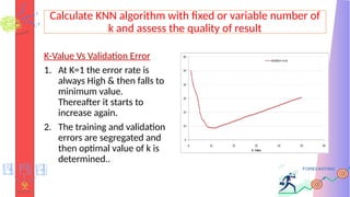
K-Value Vs Validation Error
1. At K=1 the error rate is
always High & then falls to
minimum value.
Thereafter it starts to
increase again.
2. The training and validation
errors are segregated and
then optimal value of k is
determined..
79.
Support Vector Machine(SVM)
Support Vector Machine (SVM) is a powerful machine learning
algorithm used for linear or nonlinear classification, regression,
and even outlier detection tasks.
SVMs can be used for a variety of tasks, such as text classification,
image classification, spam detection, handwriting identification,
gene expression analysis, face detection, and anomaly detection.
SVMs are adaptable and efficient in a variety of applications
because they can manage high-dimensional data and nonlinear
relationships.
80.
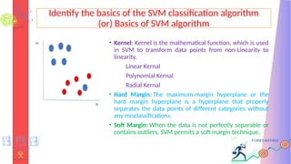
Identify the basicsof the SVM classification algorithm
(or) Basics of SVM algorithm
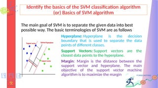
The main goal of SVM is to separate the given data into best
possible way. The basic terminologies of SVM are as follows
Hyperplane: Hyperplane is the decision
boundary that is used to separate the data
points of different classes.
Support Vectors: Support vectors are the
closest data points to the hyperplane.
Margin: Margin is the distance between the
support vector and hyperplane. The main
objective of the support vector machine
algorithm is to maximize the margin
81.
Identify the basicsof the SVM classification algorithm
(or) Basics of SVM algorithm
• Kernel: Kernel is the mathematical function, which is used
in SVM to transform data points from non-Linearity to
linearity.
Linear Kernal
Polynomial Kernal
Radial Kernal
• Hard Margin: The maximum-margin hyperplane or the
hard margin hyperplane is a hyperplane that properly
separates the data points of different categories without
any misclassifications.
• Soft Margin: When the data is not perfectly separable or
contains outliers, SVM permits a soft margin technique.
82.
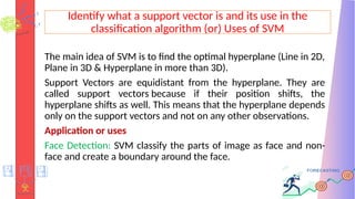
Identify what asupport vector is and its use in the
classification algorithm (or) Uses of SVM
The main idea of SVM is to find the optimal hyperplane (Line in 2D,
Plane in 3D & Hyperplane in more than 3D).
Support Vectors are equidistant from the hyperplane. They are
called support vectors because if their position shifts, the
hyperplane shifts as well. This means that the hyperplane depends
only on the support vectors and not on any other observations.
Application or uses
Face Detection: SVM classify the parts of image as face and non-
face and create a boundary around the face.
83.
Identify what asupport vector is and its use in the
classification algorithm (or) Uses of SVM
Text & Hypertext Categorization: SVM allow text and hypertext categorization
for both inductive and transductive models.
Classification of Image: SVM provides better search accuracy for image
classification.
Bio-Informatics: It includes protein classification and cancer classification. We
use SVM for identifying the classification of genes, patients on the basis of
genes and other biological problems.
Hand writing Recognition: SVM is used to detect the handwriting patterns
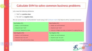
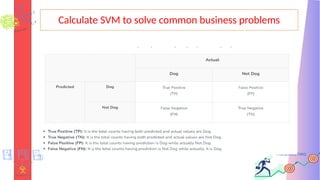
Calculate SVM tosolve common business problems
Accuracy =
Classification Error = 100 - Accuracy
87.
Identify the stepsto build a decision tree classifier
- It is a supervised Machine learning Algorithm
- Used for both regression and classification
- Builds decision nodes at each step
- Based on tree based model.
88.
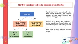
Identify the stepsto build a decision tree classifier
Root Node: It is the topmost node in the
tree, which represents the complete
dataset. It is the starting point of the
decision-making process.
Decision Node: A node that symbolizes a
choice regarding an input feature. It is
derived from parent node getting divided.
Leaf Node: A node without any child
nodes
Root Node
Internal Node (or)
Child Node (or)
Decision Node
Internal Node (or)
Child Node (or)
Decision Node
Leaf Node
(or)
Terminal Node
Leaf Node
(or)
Terminal Node
Yes No
Yes No
89.
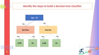
Identify the stepsto build a decision tree classifier
Age < 30
Eat Pizza
Yes
Exercise
No
Unfit
Yes
Fit
No
Unfit
Yes
Fit
No
90.
Identify the stepsto build a decision tree classifier
Step 1: A tree can be “learned” by splitting the source set into
subsets based on Attribute Selection Measures (ASM).
Step 2: This process is repeated on each derived subset in a
recursive manner called recursive partitioning
Step 3: The recursion is completed when the subset at a node all
has the same value of the target variable,
91.
Identify the stepsto build a decision tree classifier
Advantages
1. Can be used for both classification and Regression
2. Easy to interpret
3. No need for Normalization or scaling
4. Not sensitive to outliers
Disadvantages
5. Overfitting Issue
6. Small changes in the data alter the tree structure causing
instability.
7. Training time is relatively high
92.
Use a decisiontree
algorithm and appropriate metrics to solve a business problem and assess the quality of the solution
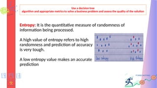
Entropy: It is the quantitative measure of randomness of
information being processed.
A high value of entropy refers to high
randomness and prediction of accuracy
is very tough.
A low entropy value makes an accurate
prediction
93.
Use a decisiontree
algorithm and appropriate metrics to solve a business problem and assess the quality of the solution
Information Gain: It is the measure of how much information a
feature provide about a class.
It gives the difference between entropy before split and average
entropy after split.
A high value of entropy refers to low information gain
A low entropy value refers to high information gain.
94.
Use a decisiontree
algorithm and appropriate metrics to solve a business problem and assess the quality of the solution
Gini Impurity: It is the measure of impurity at node.
The split made in the decision tree is said to be pure if all the data
points are accurately separated into different classes.
95.
Unit – 3: Clustering
Unsupervised Learning
Unsupervised learning is a type of machine learning that learns
from unlabeled data. This means that the data does not have any
pre-existing labels or categories. The goal of unsupervised learning
is to discover patterns and relationships in the data without any
explicit guidance. Here the task of the machine is to group
unsorted information according to similarities, patterns, and
differences without any prior training of data.
96.
Clustering
Clustering
Clustering or clusteranalysis is a machine learning technique,
which groups the unlabelled dataset. It can be defined as "A way
of grouping the data points into different clusters, consisting of
similar data points. The objects with the possible similarities
remain in a group that has less or no similarities with another
group.“
shape, size, color, behavior
cluster-ID
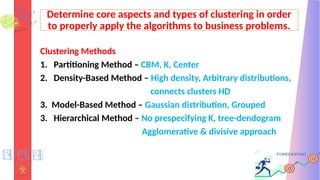
Determine core aspectsand types of clustering in order
to properly apply the algorithms to business problems.
Clustering Methods
1. Partitioning Method – CBM, K, Center
2. Density-Based Method – High density, Arbitrary distributions,
connects clusters HD
3. Model-Based Method – Gaussian distribution, Grouped
3. Hierarchical Method – No prespecifying K, tree-dendogram
Agglomerative & divisive approach
100.
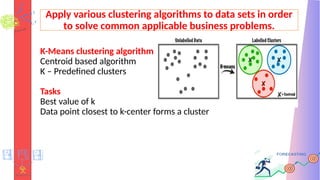
Apply various clusteringalgorithms to data sets in order
to solve common applicable business problems.
K-Means clustering algorithm
Centroid based algorithm
K – Predefined clusters
Tasks
Best value of k
Data point closest to k-center forms a cluster
101.
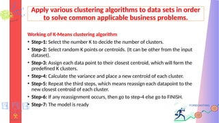
Apply various clusteringalgorithms to data sets in order
to solve common applicable business problems.
Working of K-Means clustering algorithm
• Step-1: Select the number K to decide the number of clusters.
• Step-2: Select random K points or centroids. (It can be other from the input
dataset).
• Step-3: Assign each data point to their closest centroid, which will form the
predefined K clusters.
• Step-4: Calculate the variance and place a new centroid of each cluster.
• Step-5: Repeat the third steps, which means reassign each datapoint to the
new closest centroid of each cluster.
• Step-6: If any reassignment occurs, then go to step-4 else go to FINISH.
• Step-7: The model is ready
102.
Apply various clusteringalgorithms to data sets in order
to solve common applicable business problems.
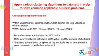
Choosing the optimum value of k
Within Cluster Sum of Squares(WCSS), which defines the total variations
within a cluster.
WCSS= Σdistance(Pi C1)2
+Σdistance(Pi C2)2
+Σdistance(Pi C3)2
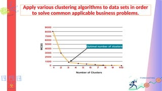
• For each value of K, calculates the WCSS value.
• Plots a curve between calculated WCSS values and the number of clusters K.
• The sharp point of bend or a point of the plot looks like an arm, then that
point is considered as the best value of K.
103.
Apply various clusteringalgorithms to data sets in order
to solve common applicable business problems.
104.
Hierarchical Clustering Algorithm
AHierarchical clustering method works via grouping data into a
tree of clusters.
Hierarchical clustering begins by treating every data point as a
separate cluster.
It iteratively combines the closest clusters until a stopping criterion
is reached.
The result of hierarchical clustering is a tree-like structure, called a
dendrogram
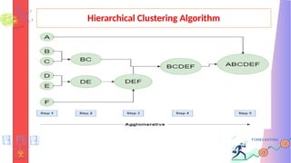
Hierarchical Clustering Algorithm
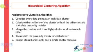
AgglomerativeClustering Algorithm
1. Consider every data point as an individual cluster
2. Calculate the similarity of one cluster with all the other clusters
(calculate proximity matrix)
3. Merge the clusters which are highly similar or close to each
other.
4. Recalculate the proximity matrix for each cluster
5. Repeat Steps 3 and 4 until only a single cluster remains.
Hierarchical Clustering Algorithm
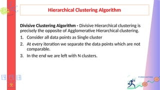
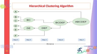
DivisiveClustering Algorithm - Divisive Hierarchical clustering is
precisely the opposite of Agglomerative Hierarchical clustering.
1. Consider all data points as Single cluster
2. At every iteration we separate the data points which are not
comparable.
3. In the end we are left with N clusters.
Hierarchical Clustering Algorithm
Advantages
•The ability to handle clusters of different sizes and densities.
• The ability to handle missing data and noisy data.
• The ability to reveal the hierarchical structure of the data, which
can be useful for understanding the relationships among the
clusters.
111.
Hierarchical Clustering Algorithm
Disadvantages
•The need for a criterion to stop the clustering process and
determine the final number of clusters.
• The computational cost is high.
• The Memory requirements of the method can be high
112.
Optimization
Optimization:
The act ofobtaining the best result under the given circumstances.
Design, construction and maintenance of engineering systems
involve decision making both at the managerial and the
technological level
Goals of such decisions :–– to minimize the effort required or to
maximize the desired benefit
113.
Optimization
Optimization:
It is definedas the process of finding the conditions that give the
minimum or maximum value of a function, where the function
represents the effort required or the desired benefit.
114.
Optimization
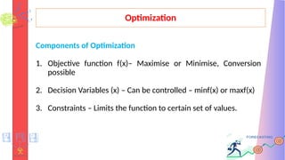
Components of Optimization
1.Objective function f(x)– Maximise or Minimise, Conversion
possible
2. Decision Variables (x) – Can be controlled – minf(x) or maxf(x)
3. Constraints – Limits the function to certain set of values.
115.
Optimization
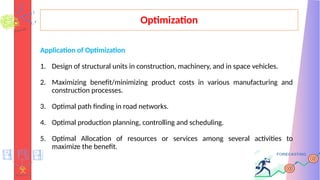
Application of Optimization
1.Design of structural units in construction, machinery, and in space vehicles.
2. Maximizing benefit/minimizing product costs in various manufacturing and
construction processes.
3. Optimal path finding in road networks.
4. Optimal production planning, controlling and scheduling.
5. Optimal Allocation of resources or services among several activities to
maximize the benefit.
116.
Optimization
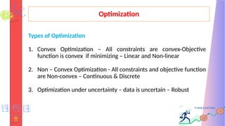
Types of Optimization
1.Convex Optimization – All constraints are convex-Objective
function is convex if minimizing – Linear and Non-linear
2. Non – Convex Optimization - All constraints and objective function
are Non-convex – Continuous & Discrete
3. Optimization under uncertainty – data is uncertain – Robust
117.
Identify the goalsand constraints of a Linear
Optimization
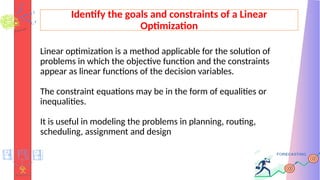
Linear optimization is a method applicable for the solution of
problems in which the objective function and the constraints
appear as linear functions of the decision variables.
The constraint equations may be in the form of equalities or
inequalities.
It is useful in modeling the problems in planning, routing,
scheduling, assignment and design
118.
Identify the goalsand constraints of a Linear
Optimization
Characteristics
• The objective function is of the minimization or maximization
type
• All the constraints are of the equality type
• All the decision variables are non-negative
119.
Identify the goalsand constraints of a Linear
Optimization
Steps of Linear Optimization
• Identify the objective function & Decision Variables.
• Identify the constraints.
• Write down the optimization model.
• Either solve graphically and/or manually else solve using R.
• Conduct sensitivity analysis.
• Interpret results and make recommendations
120.
Identify the goalsand constraints of a Linear
Optimization
Goals of Linear Optimization.
• To optimize an objective function.
• Decision variables (XX) are used to either maximize or minimize
the objective function. Examples are maximize profits, minimize
costs or time spent, minimize risks etc.
• The optimization will be w.r.t. real world quantity.
121.
Identify the goalsand constraints of a Linear
Optimization
Constraints of Linear Optimization.
• Decision variables are physical quantities under the control of
decision maker represented by Mathematical symbols. For example
X1 represents the number of kgs of product 1 produced in some
month.
• Objective function is the mathematical function of decision variables
that converts a solution into numerical evaluation.
• Constraints are functional equalities or inequalities that represents
economic, technological, numerical restrictions etc. on the decision
variables.
122.
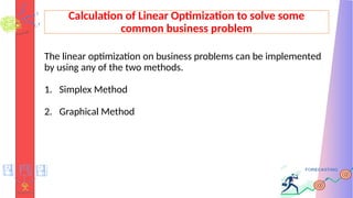
Calculation of LinearOptimization to solve some
common business problem
The linear optimization on business problems can be implemented
by using any of the two methods.
1. Simplex Method
2. Graphical Method
123.
Calculation of LinearOptimization to solve some
common business problem
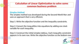
Simplex Method
The simplex method was developed during the Second World War and
uses an approach that is very efficient.
Step 1: Write the objective function and the inequality constraints.
Step 2: Convert the inequalities into equations by adding one slack
variable for each inequality.
Step 3: Construct the initial simplex tableau. Each inequality constraint
appears in its own row. Write the objective function as the bottom row.
124.
Calculation of LinearOptimization to solve some
common business problem
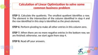
STEP 5. Calculate the quotients. The smallest quotient identifies a row.
The element in the intersection of the column identified in step 4 and
the row identified in this step is identified as the pivot element.
STEP 6. Perform pivoting to make all other entries in this column zero.
STEP 7. When there are no more negative entries in the bottom row, we
are finished; otherwise, we start again from step 4.
STEP 8. Read off your answers.
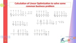
125.
Calculation of LinearOptimization to solve some
common business problem
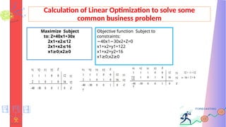
Maximize Subject
to: Z=40x1+30x
2x1+x2 12
≤
2x1+x2 16
≤
x1 0;x2 0
≥ ≥
Objective function Subject to
constraints:
−40x1 30
− x2+Z=0
x1+x2+y1=122
x1+x2+y2=16
x1 0;
≥ x2 0
≥
Simulation
Data simulation isthe process of generating synthetic data that
closely mimics the properties and characteristics of real-world data.
It is used to predict the future instance or determine the best
course of action or validate a model.
It is used to test new ideas before making a business decision.
It has the advantage of data not needing to be collected from
surveys
128.
Features of Simulation
Flexibility:
Sincethe data is manufactured, it can be adjusted to simulate a wide range of scenarios and
conditions without any constraint, allowing a system to be studied in more depth. This is
particularly useful when testing out large-scale simulation models and predictive models.
Scalability:
In addition to data quality, data volume plays a critical role in training machine learning and
artificial intelligence models. The scalability of simulated data elevates its value for such use
cases—since the data is artificial, it can be generated as needed to reflect the randomness and
complexity of real-world systems.
Replicability:
Similar circumstances and conditions can be reproduced in a different simulated dataset to
ensure consistency in testing. This consistency is crucial for validating models and hypotheses,
as it allows you to test them repeatedly and refine them based on the results.
129.
Advantages or Benefitsor Usecase of Simulation
Enhanced Decision Making:
Data simulation can inform decision-making by simulating various conditions or events and predicting
outcomes based on actions.
Cost Efficiency:
The harvested data is more cost-effective, as it reduces the need for physical testing and active data
collection. Hence the cost is reduced.
Improved Model Validity
Data simulation can aid in model testing and refinement. Creating a virtual representation of a real-
world system makes it possible to test different models and refine them based on the results, leading
to more accurate models that are better at predicting scenarios in great detail.
Risk Reduction
Data simulation can provide data on crises and potential issues, allowing organizations to identify
pitfalls or challenges before they occur in the real world. This can avoid risks in the long term run.
130.
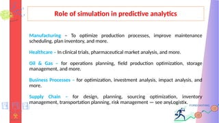
Role of simulationin predictive analytics
Manufacturing – To optimize production processes, improve maintenance
scheduling, plan inventory, and more.
Healthcare – In clinical trials, pharmaceutical market analysis, and more.
Oil & Gas – for operations planning, field production optimization, storage
management, and more.
Business Processes – for optimization, investment analysis, impact analysis, and
more.
Supply Chain – for design, planning, sourcing optimization, inventory
management, transportation planning, risk management — see anyLogistix.
131.
Types of simulation
MonteCarlo simulations. It uses random sampling to obtain results
for uncertain situations and is widely used in finance, physics, and
engineering to model complex systems and predict behavior.
Agent-based modeling. This type of simulation focuses on the actions
and interactions of individual & autonomous agents within the data
systems.
System dynamics: System dynamics helps to understand non-linear
feedback loops in more complex systems and is often used in
economics, environmental science etc
132.
Types of simulation
•Discrete-event simulations: These models focus on individual
events in the system and how they affect the outcome, and are
widely used in operations research, computer science, and
logistics to simulate processes and systems.
133.
Monte Carlo Simulation
•Monte Carlo simulation is a technique in which random numbers are
substituted into a statistical model in order to forecast the future values.
Step 1: Define the Problem
Define – Identify Objectives – Factors impact on objectives
Step 2: Construct an appropriate model
Variables & Parameters – Appropriate decision rules
Type of distribution – relation b/w variables & parameters
134.
Monte Carlo Simulation
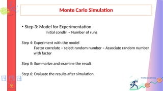
•Step 3: Model for Experimentation
Initial condtn – Number of runs
Step 4: Experiment with the model
Factor correlate – select random number – Associate random number
with factor
Step 5: Summarize and examine the result
Step 6: Evaluate the results after simulation.
135.
Naïve Bayes algorithm
•Bayes theorem, named after Thomas Bayes from the 1700s. The
Naive Bayes classifier works on the principle of conditional
probability, as given by the Bayes theorem.
• Consider the following example of tossing two coins. If we toss
two coins and look at all the different possibilities, we have the
sample space as:{HH, HT, TH, TT}
136.
Naïve Bayes algorithm
•The probability of getting two heads = 1/4
• The probability of at least one tail = 3/4
• The probability of the second coin being head given the first coin
is tail = 1/2
• The probability of getting two heads given the first coin is a head
= ½
137.
Naïve Bayes algorithm
•The Bayes theorem gives us the conditional probability of event
A, given that event B has occurred. In this case, the first coin toss
will be B and the second coin toss A.
• Now in this sample space, let A be the event that the second coin
is head, and B be the event that the first coin is tails
• We're going to focus on A, and we write that out as a probability
of A given B:
P(A|B) = [ P(B|A) * P(A) ] / P(B)
138.
Naïve Bayes algorithm
•= [ P(First coin being tail given the second coin is the head) *
P(Second coin being head) ] / P(First coin being tail)
• = [ (1/2) * (1/2) ] / (1/2)
• = 1/2 = 0.5


![Naïve Bayes algorithm
• The Bayes theorem gives us the conditional probability of event
A, given that event B has occurred. In this case, the first coin toss
will be B and the second coin toss A.
• Now in this sample space, let A be the event that the second coin
is head, and B be the event that the first coin is tails
• We're going to focus on A, and we write that out as a probability
of A given B:
P(A|B) = [ P(B|A) * P(A) ] / P(B)](https://image.slidesharecdn.com/fpaas-250327084415-a440583a/85/Forecasting-Using-the-Predictive-Analytics-137-320.jpg)
![Naïve Bayes algorithm
• = [ P(First coin being tail given the second coin is the head) *
P(Second coin being head) ] / P(First coin being tail)
• = [ (1/2) * (1/2) ] / (1/2)
• = 1/2 = 0.5](https://image.slidesharecdn.com/fpaas-250327084415-a440583a/85/Forecasting-Using-the-Predictive-Analytics-138-320.jpg)