Downloaded 13 times
![Prepared by Volkan OBAN
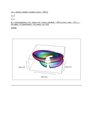
Advanced Data Visualization in R- Somes Examples.
geomorph package in R....
Example:
Code:
>library(geomorph)
> data(scallopPLY)
> ply <- scallopPLY$ply
> digitdat <- scallopPLY$coords
> plotspec(spec=ply,digitspec=digitdat,fixed=16, centered =TRUE)
Example:
> data(scallops)
> Y.gpa<-gpagen(A=scallops$coorddata, curves=scallops$curvslide,
surfaces=scallops$surfslide)
> ref<-mshape(Y.gpa$coords)
> plotRefToTarget(ref,Y.gpa$coords[,,1],method="TPS", mag=3)](https://image.slidesharecdn.com/geomorphpackageinr-160926131355/85/Advanced-Data-Visualization-in-R-Somes-Examples-1-320.jpg)

![+ # constrained by y >= (.25 quantile) - range.wisk*Interquartile rang
e
+
+ Q <- quantile(y, c(0.25, 0.5, 0.75))
+ names(Q) <- NULL # gets rid of percentages
+ IQ.range <- Q[3] - Q[1]
+ low <- Q[1] - range.wisk * IQ.range
+ high <- Q[3] + range.wisk * IQ.range
+ index <- which((y >= low) & (y <= high))
+ wisk.low <- min(y[index])
+ wisk.high <- max(y[index])
+ outliers <- y[which((y < low) | (y > high))]
+
+ # plot median:
+ points(xloc, Q[2], pch = pch.box, cex = cex.boxpoint, col = color)
+
+ # plot box:
+ xleft <- xloc - width.box/2
+ xright <- xloc + width.box/2
+ ybottom <- Q[1]
+ ytop <- Q[3]
+ rect(xleft, ybottom, xright, ytop, lwd = lwd.box, border = color)
+
+ # plot whiskers:
+ segments(xloc, wisk.low, xloc, Q[1], lwd = lwd.wisk, col = color)
+ segments(xloc, Q[3], xloc, wisk.high, lwd = lwd.wisk, col = color)
+
+ # plot horizontal segments:
+ x0 <- xloc - width.hor/2
+ x1 <- xloc + width.hor/2
+ segments(x0, wisk.low, x1, wisk.low, lwd = lwd.hor, col = color)
+ segments(x0, wisk.high, x1, wisk.high, lwd = lwd.hor, col = color)
+
+ # plot outliers:
+ if (plot.outliers == TRUE) {
+ xloc.p <- rep(xloc, length(outliers))
+ points(xloc.p, outliers, pch = pch.out, cex = cex.out, col = col
or)
+ }
+ }
>
> RT.hf.sp <- rnorm(1000, mean = 0.41, sd = 0.008)
> RT.lf.sp <- rnorm(1000, mean = 0.43, sd = 0.01)
> RT.vlf.sp <- rnorm(1000, mean = 0.425, sd = 0.012)
> RT.hf.ac <- rnorm(1000, mean = 0.46, sd = 0.008)
> RT.lf.ac <- rnorm(1000, mean = 0.51, sd = 0.01)
> RT.vlf.ac <- rnorm(1000, mean = 0.52, sd = 0.012)
>
> ps <- 1 # size of boxpoint
> par(cex.main = 1.5, mar = c(5, 6, 4, 5) + 0.1, mgp = c(3.5, 1, 0), cex.l
ab = 1.5,
+ font.lab = 2, cex.axis = 1.3, bty = "n", las = 1)
> x <- c(1, 2, 3, 4)
> plot(x, c(-10, -10, -10, -10), type = "p", ylab = " ", xlab = " ", cex =
1.5,
+ ylim = c(0.3, 0.6), xlim = c(1, 4), lwd = 2, pch = 5, axes = FALSE,
main = " ")
> axis(1, at = c(1.5, 2.5, 3.5), labels = c("HF", "LF", "VLF"))
> mtext("Word Frequency", side = 1, line = 3, cex = 1.5, font = 2)
> axis(2, pos = 1.1)
> par(las = 0)
> mtext("Group Mean M", side = 2, line = 2.9, cex = 1.5, font = 2)
>
> x <- c(1.5, 2.5, 3.5)
> boxplot.ej(RT.hf.sp, xloc = 1.5, cex.boxpoint = ps)
> boxplot.ej(RT.hf.ac, xloc = 1.5, cex.boxpoint = ps, color = "grey")
> boxplot.ej(RT.lf.sp, xloc = 2.5, cex.boxpoint = ps)
> boxplot.ej(RT.lf.ac, xloc = 2.5, cex.boxpoint = ps, color = "grey")
> boxplot.ej(RT.vlf.sp, xloc = 3.5, cex.boxpoint = ps)](https://image.slidesharecdn.com/geomorphpackageinr-160926131355/85/Advanced-Data-Visualization-in-R-Somes-Examples-3-320.jpg)

![+ at <- 1:n
+ # pass 1 - calculate base range - estimate density setup parameters
for
+ # density estimation
+ upper <- vector(mode = "numeric", length = n)
+ lower <- vector(mode = "numeric", length = n)
+ q1 <- vector(mode = "numeric", length = n)
+ q3 <- vector(mode = "numeric", length = n)
+ med <- vector(mode = "numeric", length = n)
+ base <- vector(mode = "list", length = n)
+ height <- vector(mode = "list", length = n)
+ outliers <- vector(mode = "list", length = n)
+ baserange <- c(Inf, -Inf)
+
+ # global args for sm.density function-call
+ args <- list(display = "none")
+
+ if (!(is.null(h)))
+ args <- c(args, h = h)
+ for (i in 1:n) {
+ data <- datas[[i]]
+ if (!is.null(ids))
+ names(data) <- ids
+ if (is.null(names(data)))
+ names(data) <- as.character(1:(length(data)))
+
+ # calculate plot parameters 1- and 3-quantile, median, IQR, uppe
r- and
+ # lower-adjacent
+ data.min <- min(data)
+ data.max <- max(data)
+ q1[i] <- quantile(data, 0.25)
+ q3[i] <- quantile(data, 0.75)
+ med[i] <- median(data)
+ iqd <- q3[i] - q1[i]
+ upper[i] <- min(q3[i] + range * iqd, data.max)
+ lower[i] <- max(q1[i] - range * iqd, data.min)
+
+ # strategy: xmin = min(lower, data.min)) ymax = max(upper, data.
max))
+ est.xlim <- c(min(lower[i], data.min), max(upper[i], data.max))
+
+ # estimate density curve
+ smout <- do.call("sm.density", c(list(data, xlim = est.xlim), ar
gs))
+
+ # calculate stretch factor the plots density heights is defined
in range 0.0
+ # ... 0.5 we scale maximum estimated point to 0.4 per data
+ hscale <- 0.4/max(smout$estimate) * wex
+
+ # add density curve x,y pair to lists
+ base[[i]] <- smout$eval.points
+ height[[i]] <- smout$estimate * hscale
+ t <- range(base[[i]])
+ baserange[1] <- min(baserange[1], t[1])
+ baserange[2] <- max(baserange[2], t[2])
+ min.d <- boxplot.stats(data)[["stats"]][1]
+ max.d <- boxplot.stats(data)[["stats"]][5]
+ height[[i]] <- height[[i]][(base[[i]] > min.d) & (base[[i]] < ma
x.d)]
+ height[[i]] <- c(height[[i]][1], height[[i]], height[[i]][length
(height[[i]])])
+ base[[i]] <- base[[i]][(base[[i]] > min.d) & (base[[i]] < max.d)
]
+ base[[i]] <- c(min.d, base[[i]], max.d)
+ outliers[[i]] <- list(data[(data < min.d) | (data > max.d)], nam
es(data[(data <](https://image.slidesharecdn.com/geomorphpackageinr-160926131355/85/Advanced-Data-Visualization-in-R-Somes-Examples-5-320.jpg)
![+
min.d) | (data > max.d)]))
+
+ # calculate min,max base ranges
+ }
+ # pass 2 - plot graphics setup parameters for plot
+ if (!add) {
+ xlim <- if (n == 1)
+ at + c(-0.5, 0.5) else range(at) + min(diff(at))/2 * c(-1, 1
)
+
+ if (is.null(ylim)) {
+ ylim <- baserange
+ }
+ }
+ if (is.null(names)) {
+ label <- 1:n
+ } else {
+ label <- names
+ }
+ boxwidth <- 0.05 * wex
+
+ # setup plot
+ if (!add)
+ plot.new()
+ if (!horizontal) {
+ if (!add) {
+ plot.window(xlim = xlim, ylim = ylim)
+ axis(2)
+ axis(1, at = at, label = label)
+ }
+
+ box()
+ for (i in 1:n) {
+ # plot left/right density curve
+ polygon(c(at[i] - height[[i]], rev(at[i] + height[[i]])), c(
base[[i]],
+
rev(base[[i]])), col = col, border = border, lty = lty, lwd = lwd)
+
+ if (drawRect) {
+ # browser() plot IQR
+ boxplot(datas[[i]], at = at[i], add = TRUE, yaxt = yaxt,
pars = list(boxwex = 0.6 *
+
wex, outpch = if (mark.outlier) "" else 1))
+ if ((length(outliers[[i]][[1]]) > 0) & mark.outlier)
+ text(rep(at[i], length(outliers[[i]][[1]])), outlier
s[[i]][[1]],
+ labels = outliers[[i]][[2]])
+ # lines( at[c( i, i)], c(lower[i], upper[i]) ,lwd=lwd, l
ty=lty) plot 50% KI
+ # box rect( at[i]-boxwidth/2, q1[i], at[i]+boxwidth/2, q
3[i], col=rectCol)
+ # plot median point points( at[i], med[i], pch=pchMed, c
ol=colMed )
+ }
+ points(at[i], mean(datas[[i]]), pch = pch.mean, cex = 1.3)
+ }
+ } else {
+ if (!add) {
+ plot.window(xlim = ylim, ylim = xlim)
+ axis(1)
+ axis(2, at = at, label = label)
+ }
+
+ box()
+ for (i in 1:n) {
+ # plot left/right density curve](https://image.slidesharecdn.com/geomorphpackageinr-160926131355/85/Advanced-Data-Visualization-in-R-Somes-Examples-6-320.jpg)
![+ polygon(c(base[[i]], rev(base[[i]])), c(at[i] - height[[i]],
rev(at[i] +
+
height[[i]])), col = col, border = border, lty = lty, lwd = lwd)
+
+ if (drawRect) {
+ # plot IQR
+ boxplot(datas[[i]], yaxt = yaxt, at = at[i], add = TRUE,
pars = list(boxwex = 0.8 *
+
wex, outpch = if (mark.outlier) "" else 1))
+ if ((length(outliers[[i]][[1]]) > 0) & mark.outlier)
+ text(rep(at[i], length(outliers[[i]][[1]])), outlier
s[[i]][[1]],
+ labels = outliers[[i]][[2]])
+ # lines( at[c( i, i)], c(lower[i], upper[i]) ,lwd=lwd, l
ty=lty)
+ }
+ points(at[i], mean(datas[[i]]), pch = pch.mean, cex = 1.3)
+ }
+ }
+ invisible(list(upper = upper, lower = lower, median = med, q1 = q1,
q3 = q3))
+ }
>
> # plot
> par(cex.main = 1.5, mar = c(5, 6, 4, 5) + 0.1, mgp = c(3.5, 1, 0), cex.l
ab = 1.5,
+ font.lab = 2, cex.axis = 1.3, bty = "n", las = 1)
> x <- c(1, 2, 3, 4)
> plot(x, c(-10, -10, -10, -10), type = "p", ylab = " ", xlab = " ", cex =
1.5,
+ ylim = c(0.3, 0.6), xlim = c(1, 4), lwd = 2, pch = 5, axes = F, mai
n = " ")
> axis(1, at = c(1.5, 2.5, 3.5), labels = c("HF", "LF", "VLF"))
> axis(2, pos = 1.1)
> mtext("Word Frequency", side = 1, line = 3, cex = 1.5, font = 2)
>
> par(las = 0)
> mtext("Group Mean M", side = 2, line = 2.9, cex = 1.5, font = 2)
>
> x <- c(1.5, 2.5, 3.5)
>
> vioplot.singmann(RT.hf.sp, RT.lf.sp, RT.vlf.sp, add = TRUE, mark.outlier
= FALSE,
+ at = c(1.5, 2.5, 3.5), wex = 0.4, yaxt = "n")
> vioplot.singmann(RT.hf.ac, RT.lf.ac, RT.vlf.ac, add = TRUE, mark.outlier
= FALSE,
+ at = c(1.5, 2.5, 3.5), wex = 0.4, col = "grey", border
= "grey", rectCol = "grey",
+ colMed = "grey", yaxt = "n")
>
> text(2.5, 0.35, "Speed", cex = 1.4, font = 1, adj = 0.5)
> text(2.5, 0.58, "Accuracy", cex = 1.4, font = 1, col = "grey", adj = 0.5
)](https://image.slidesharecdn.com/geomorphpackageinr-160926131355/85/Advanced-Data-Visualization-in-R-Somes-Examples-7-320.jpg)

![points(x, MRT, cex = 1.5, lwd = 2, pch = 19)
plot.errbars = plotsegraph(x, MRT, MRT.se, 0.1, color = "black") #0.1 = wi
skwidth
lines(c(1.5, 2.5, 3.5), MRT, lwd = 2, type = "c")
text(1.5, MRT[1] + 60, "429", adj = 0.5, cex = digitsize)
text(2.5, MRT[2] + 60, "515", adj = 0.5, cex = digitsize)
text(3.5, MRT[3] + 60, "555", adj = 0.5, cex = digitsize)
par(new = TRUE)
x <- c(1, 2, 3, 4)
plot(x, c(-10, -10, -10, -10), type = "p", ylab = " ", xlab = " ", cex = 1.
5,
ylim = c(0, 1), xlim = c(1, 4), lwd = 2, axes = FALSE, main = " ")
axis(4, at = c(0, 0.1, 0.2, 0.3, 0.4), las = 1)
grid::grid.text("Mean Proportion of Errors", 0.97, 0.5, rot = 270, gp = gri
d::gpar(cex = 1.5,
font = 2))
width <- 0.25
linewidth <- 2
x0 <- 1.5 - width
x1 <- 1.5 + width
y0 <- 0
y1 <- Er[1]
segments(x0, y0, x0, y1, lwd = linewidth)
segments(x0, y1, x1, y1, lwd = linewidth)
segments(x1, y1, x1, y0, lwd = linewidth)
segments(x1, y0, x0, y0, lwd = linewidth)
x0 <- 2.5 - width
x1 <- 2.5 + width
y0 <- 0
y1 <- Er[2]
segments(x0, y0, x0, y1, lwd = linewidth)
segments(x0, y1, x1, y1, lwd = linewidth)
segments(x1, y1, x1, y0, lwd = linewidth)
segments(x1, y0, x0, y0, lwd = linewidth)](https://image.slidesharecdn.com/geomorphpackageinr-160926131355/85/Advanced-Data-Visualization-in-R-Somes-Examples-10-320.jpg)
![x0 <- 3.5 - width
x1 <- 3.5 + width
y0 <- 0
y1 <- Er[3]
segments(x0, y0, x0, y1, lwd = linewidth)
segments(x0, y1, x1, y1, lwd = linewidth)
segments(x1, y1, x1, y0, lwd = linewidth)
segments(x1, y0, x0, y0, lwd = linewidth)
loc.errbars <- c(1.5, 2.5, 3.5)
plot.errbars <- plotsebargraph(loc.errbars, Er, Er.se, 0.2, color = "black"
) # 0.2 = wiskwidth
text(1.5, 0.9, "Behavioral Data", font = 2, cex = 2, pos = 4)
text(1.5, 0.05, "0.23", adj = 0.5, cex = digitsize)
text(2.5, 0.05, "0.14", adj = 0.5, cex = digitsize)
text(3.5, 0.05, "0.13", adj = 0.5, cex = digitsize)](https://image.slidesharecdn.com/geomorphpackageinr-160926131355/85/Advanced-Data-Visualization-in-R-Somes-Examples-11-320.jpg)
![text(7.5, L2, expression(paste(italic("L"), " = .32")), adj = 0, col = "red
4",
cex = 1.8)
text(-16, 0.35, expression(paste(H[0], " : ", mu[diff], " = 0", sep = "")),
adj = 0,
cex = 1.8)
text(-16, 0.3, expression(paste(H[1], " : ", mu[diff], " = 9", sep = "")),
adj = 0,
cex = 1.8)
mtext(expression(bar(x)[diff]), side = 1, line = 2, at = 6.5, adj = 0, col
= "red4",
cex = 1.8, padj = 0.1)
text(14, 0.2, expression(paste("LR = ", frac(".32", ".04") %~~% 8, sep = ""
)),
adj = 0, col = "red4", cex = 1.8)
Example:](https://image.slidesharecdn.com/geomorphpackageinr-160926131355/85/Advanced-Data-Visualization-in-R-Somes-Examples-13-320.jpg)
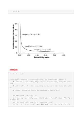
![Max.BF10 = function(p) {
# Computes the upper bound on the Bayes factor As in Sellke, Bayarri, &
# Berger, 2001
Max.BF10 <- -1/(exp(1) * p * log(p))
return(Max.BF10)
}
# Plot this function for p in .001 to .1
xlow <- 0.001
xhigh <- 0.1
p1 <- 0.0373
p2 <- 0.00752
p3 <- 0.001968
par(cex.main = 1.5, mar = c(5, 6, 4, 5) + 0.1, mgp = c(3.5, 1, 0), cex.lab
= 1.5,
font.lab = 2, cex.axis = 1.3, bty = "n", las = 1)
plot(function(p) Max.BF10(p), xlow, xhigh, xlim = c(xlow, xhigh), lwd = 2,
xlab = " ",
ylab = " ")
mtext("Two-sided p value", 1, line = 2.5, cex = 1.5, font = 2)
mtext("Maximum Bayes factor for H1", 2, line = 2.8, cex = 1.5, font = 2, la
s = 0)
lines(c(0, p1), c(3, 3), lwd = 2, col = "grey")
lines(c(0, p2), c(10, 10), lwd = 2, col = "grey")
lines(c(0, p3), c(30, 30), lwd = 2, col = "grey")
lines(c(p1, p1), c(0, 3), lwd = 2, col = "grey")
lines(c(p2, p2), c(0, 10), lwd = 2, col = "grey")
lines(c(p3, p3), c(0, 30), lwd = 2, col = "grey")
cexsize <- 1.2
text(0.005, 31, expression(max((BF[10])) == 30 %<->% p %~~% 0.002), cex = c
exsize,
pos = 4)
text(0.01, 11, expression(max((BF[10])) == 10 %<->% p %~~% 0.008), cex = ce
xsize,
pos = 4)
text(p1 - 0.005, 5, expression(max((BF[10])) == 3 %<->% p %~~% 0.037), cex
= cexsize,](https://image.slidesharecdn.com/geomorphpackageinr-160926131355/85/Advanced-Data-Visualization-in-R-Somes-Examples-14-320.jpg)
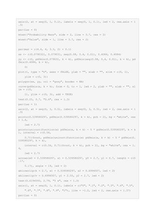
![if (show.losses == TRUE) {
index.losses <- which(lo < 0)
points(matrix(c(index.losses, choice[index.losses]), byrow = FALSE,
nrow = length(index.losses)),
pch = 19, lwd = 1.5)
}
}
# Synthetic data
choice <- sample(1:4, 100, replace = TRUE)
lo <- sample(c(-1250, -250, -50, 0), 100, replace = TRUE)
# postscript('DiversePerformance.eps', width = 7, height = 7)
IndividualPerformance(choice, lo, show.losses = TRUE)
# dev.off()](https://image.slidesharecdn.com/geomorphpackageinr-160926131355/85/Advanced-Data-Visualization-in-R-Somes-Examples-16-320.jpg)
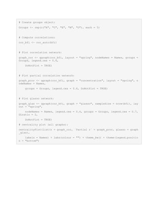
![Example:
library(plotrix)
# mix of 2 normal distributions
mixedNorm <- function(x) {
return(0.5 * dnorm(x, 0.25, 0.13) + 0.5 * dnorm(x, 0.7, 0.082))
}
### normalize so that area [0,1] integrates to 1; k = normalizing constant
k <- 1/integrate(mixedNorm, 0, 1)$value
# normalized
pdfmix <- function(x, k) {
return(k * (0.5 * dnorm(x, 0.25, 0.13) + 0.5 * dnorm(x, 0.7, 0.082)))
}
# integrate(pdfmix, 0.0790321,0.4048)$value # 0.4
op <- par(mfrow = c(1, 2), mar = c(5.9, 6, 4, 2) + 0.1)
barplot(height = c(0.2, 0.25, 0.1, 0.05, 0.35, 0.05), names.arg = c(1,
2, 3, 4, 5, 6), axes = FALSE, ylim = c(0, 1), width = 1, cex.names = 1.
5)
arrows(x0 = 0.6, x1 = 0.6, y0 = 0.38, y1 = 0.23, length = c(0.2, 0.2),
lwd = 2)
text(0.6, 0.41, "0.2", cex = 1.3)
ablineclip(v = 1.9, y1 = 0.28, y2 = 0.375, lwd = 2)
ablineclip(v = 4.2, y1 = 0.28, y2 = 0.375, lwd = 2)
ablineclip(h = 0.375, x1 = 1.9, x2 = 4.2, lwd = 2)
arrows(x0 = 3.05, x1 = 3.05, y0 = 0.525, y1 = 0.375, length = c(0.2, 0.2),
lwd = 2)
text(3.05, 0.555, "0.4", cex = 1.3)
ablineclip(v = 5.5, y1 = 0.38, y2 = 0.43, lwd = 2)
arrows(x0 = 6.7, x1 = 6.7, y0 = 0.43, y1 = 0.09, length = c(0.2, 0.2),
lwd = 2)
ablineclip(h = 0.43, x1 = 5.5, x2 = 6.7, lwd = 2)
text(6.1, 0.46, "7 x", cex = 1.3)
par(las = 1)](https://image.slidesharecdn.com/geomorphpackageinr-160926131355/85/Advanced-Data-Visualization-in-R-Somes-Examples-17-320.jpg)
![mtext("Probability Density", side = 2, line = 3.7, cex = 2)
mtext("Value", side = 1, line = 2.4, cex = 2)
par(op)
Example:
library("psych")
library("qgraph")
# Load BFI data:
data(bfi)
bfi <- bfi[, 1:25]
# Groups and names object (not needed really, but make the plots easier to
# interpret):
Names <- scan("http://sachaepskamp.com/files/BFIitems.txt", what = "charact
er", sep = "n")](https://image.slidesharecdn.com/geomorphpackageinr-160926131355/85/Advanced-Data-Visualization-in-R-Somes-Examples-19-320.jpg)
![cex.labels <- 1.3
cexLegend <- 1.2
op <- par(mar = c(5.1, 4.1, 4.1, 2.1))
### create empty canvas
plot(1, xlim = xlim, ylim = ylim, axes = FALSE, xlab = "", ylab = "")
### shade prior area < 70
greycol1 <- rgb(0, 0, 0, alpha = 0.2)
greycol2 <- rgb(0, 0, 0, alpha = 0.4)
polPrior <- seq(xlim[1], 70, length.out = 400)
xx <- c(polPrior, polPrior[length(polPrior)], polPrior[1])
yy <- c(dnorm(polPrior, mean.prior, sd.prior), 0, 0)
polygon(xx, yy, col = greycol1, border = NA)
### shade posterior area < 70
polPosterior <- seq(xlim[1], 70, length.out = 400)
xx <- c(polPosterior, polPosterior[length(polPosterior)], polPosterior[1])
yy <- c(dnorm(polPosterior, mean.posterior, sd.posterior), 0, 0)
polygon(xx, yy, col = greycol2, border = NA)
### shade posterior area on interval (81, 84)
polPosterior2 <- seq(81, 84, length.out = 400)
xx <- c(polPosterior2, polPosterior2[length(polPosterior2)], polPosterior2[
1])
yy <- c(dnorm(polPosterior2, mean.posterior, sd.posterior), 0, 0)
polygon(xx, yy, col = greycol2, border = NA)
### grey dashed lines to prior mean, posterior mean and posterior at 77
lines(rep(mean.prior, 2), c(0, dnorm(mean.prior, mean.prior, sd.prior)), lt
y = 2, col = "grey",
lwd = lwd)
lines(rep(mean.posterior, 2), c(0, dnorm(mean.posterior, mean.posterior, sd
.posterior)),
lty = 2, col = "grey", lwd = lwd)](https://image.slidesharecdn.com/geomorphpackageinr-160926131355/85/Advanced-Data-Visualization-in-R-Somes-Examples-22-320.jpg)
![lines(rep(mean.posterior + (mean.posterior - 70), 2), c(0, dnorm(mean.poste
rior + (mean.posterior -
70), mean.posterior, sd.posterior)), lty = 2, col = "grey", lwd = lwd)
### axes
axis(1, at = seq(xlim[1], xlim[2], 5), cex.axis = cex.axis, lwd = lwd.axis)
axis(2, labels = FALSE, tck = 0, lwd = lwd.axis, line = -0.5)
### axes labels
mtext("IQ Bob", side = 1, cex = 1.6, line = 2.4)
mtext("Density", side = 2, cex = 1.5, line = 0)
### plot prior and posterior
# prior
plot(function(x) dnorm(x, mean.prior, sd.prior), xlim = xlim, ylim = ylim,
xlab = "",
ylab = "", lwd = lwd, lty = 3, add = TRUE)
# posterior
plot(function(x) dnorm(x, mean.posterior, sd.posterior), xlim = xlim, ylim
= ylim, add = TRUE,
lwd = lwd)
### add points
# posterior density at 70
points(70, dnorm(70, mean.posterior, sd.posterior), pch = 21, bg = "white",
cex = cex.points,
lwd = lwd.points)
# posterior density at 76.67
points(mean.posterior + (mean.posterior - 70), dnorm(mean.posterior + (mean
.posterior -
70), mean.posterior, sd.posterior), pch = 21, bg = "white", cex = cex.p
oints, lwd = lwd.points)
# maximum a posteriori value](https://image.slidesharecdn.com/geomorphpackageinr-160926131355/85/Advanced-Data-Visualization-in-R-Somes-Examples-23-320.jpg)
![points(mean.posterior, dnorm(mean.posterior, mean.posterior, sd.posterior),
pch = 21,
bg = "white", cex = cex.points, lwd = lwd.points)
### credible interval
CIlow <- qnorm(0.025, mean.posterior, sd.posterior)
CIhigh <- qnorm(0.975, mean.posterior, sd.posterior)
yCI <- 0.11
arrows(CIlow, yCI, CIhigh, yCI, angle = 90, code = 3, length = 0.1, lwd = l
wd)
text(mean.posterior, yCI + 0.0042, labels = "95%", cex = cex.text)
text(CIlow, yCI, labels = paste(round(CIlow, 2)), cex = cex.text, pos = 2,
offset = 0.3)
text(CIhigh, yCI, labels = paste(round(CIhigh, 2)), cex = cex.text, pos = 4
, offset = 0.3)
### legend
legendPosition <- 115
legend(legendPosition, ylim[2] + 0.002, legend = c("Posterior", "Prior"), l
ty = c(1,
3), bty = "n", lwd = c(lwd, lwd), cex = cexLegend, xjust = 1, yjust = 1
, x.intersp = 0.6,
seg.len = 1.2)
### draw labels
# A
arrows(x0 = 57, x1 = 61, y0 = dnorm(62, mean.prior, sd.prior) + 0.0003, y1
= dnorm(62,
mean.prior, sd.prior) - 0.007, length = c(0.08, 0.08), lwd = lwd, code
= 2)
text(55.94, dnorm(5, mean.prior, sd.prior) + 0.0205, labels = "A", cex = ce
x.labels)
# B
arrows(x0 = 64.5, x1 = 69, y0 = dnorm(68, mean.posterior, sd.posterior) + 0
.003, y1 = dnorm(68,
mean.posterior, sd.posterior) - 0.005, length = c(0.08, 0.08), lwd = lw
d, code = 2)](https://image.slidesharecdn.com/geomorphpackageinr-160926131355/85/Advanced-Data-Visualization-in-R-Somes-Examples-24-320.jpg)
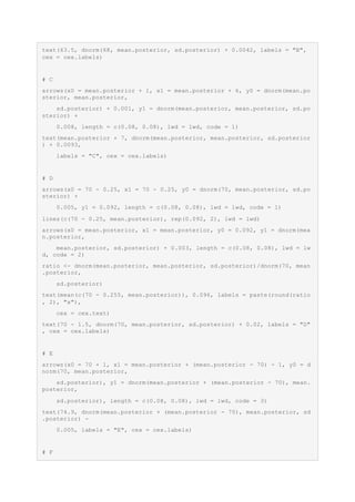

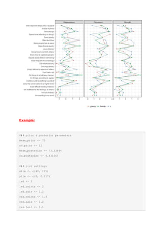
![> forest(x = g, sei = gSE, xlab = "Hedges' g", cex.lab = 1.4, ilab = cbind(
cMeanSmile,
+
cMeanPout), ilab.xpos = c(-3.2, -2.5), cex.axis = 1.1, mlab = "Meta-Analyti
c Effect:",
+ lwd = 1.4, rows = 22:2, addfit = FALSE, atransf = FALSE, ylim = c(
-2, 25))
There were 50 or more warnings (use warnings() to see the first 50)
>
> text(-4.05, 24, "Study", cex = 1.3)
> text(-3.2, 24, "Smile", cex = 1.3)
> text(-2.5, 24, "Pout", cex = 1.3)
> text(2.75, 24, "Hedges' g [95% CI]", cex = 1.3)
>
> abline(h = 1, lwd = 1.4)
> addpoly(metaG, atransf = FALSE, row = -1, cex = 1.3, mlab = "Meta-Analyti
c Effect Size:")
Reference: http://shinyapps.org/apps/RGraphCompendium/index.php
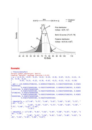
Example:
> library(tidyr)
> library(plotly)
> s <- read.csv("https://raw.githubusercontent.com/plotly/datasets/master/s
chool_earnings.csv")
> s <- s[order(s$Men), ]
> gather(s, Sex, value, Women, Men) %>%
+ plot_ly(x = value, y = School, mode = "markers",
+ color = Sex, colors = c("pink", "blue")) %>%
+ add_trace(x = value, y = School, mode = "lines",](https://image.slidesharecdn.com/geomorphpackageinr-160926131355/85/Advanced-Data-Visualization-in-R-Somes-Examples-28-320.jpg)

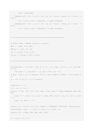
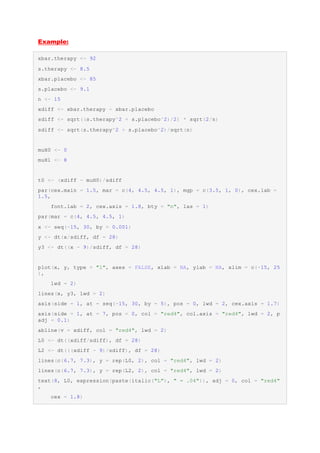
This document provides examples of using the geomorph package in R for advanced data visualization. It includes code snippets showing how to visualize geometric morphometric data using functions like plotspec() and plotRefToTarget(). It also includes an example of creating a customized violin plot function for comparing multiple groups and generating simulated data to plot.


![Some R Examples[R table and Graphics] -Advanced Data Visualization in R (Some...](https://cdn.slidesharecdn.com/ss_thumbnails/exampless-160922204223-thumbnail.jpg?width=640&height=640&fit=bounds)


![Some Examples in R- [Data Visualization--R graphics]](https://cdn.slidesharecdn.com/ss_thumbnails/rchart-160729210112-thumbnail.jpg?width=640&height=640&fit=bounds)