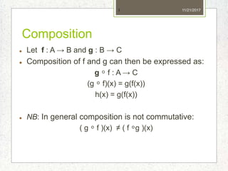
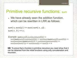
The document discusses primitive recursive functions and predicates. It defines primitive recursive functions as those that can be constructed from initial functions using only composition and recursion. Some examples of primitive recursive functions given are addition, multiplication, factorial, power, predecessor, absolute value, and bounded quantification. Predicates like equality, less than, negation, conjunction, disjunction, division, and primality are also shown to be primitive recursive. The concept of bounded minimalization is introduced, where a function returns the least value t for which a primitive recursive predicate P(t,x1,...xn) is true.

1. Primitive
Recursive
Functions
-Sampath Kumar S,
AP/CSE, SECE
11/21/2017
1

2. Preliminaries: partial and total functions
 The domain of a partial function on set A contains the subset of A.
 The domain of a total function on set A contains the entire set A.
 A partial function f is called partially computable if there
is some program that computes it. Another term for such
functions partial recursive.
 Similarly, a function f is called computable if it is both
total and partially computable. Another term for such
function is recursive.
2 11/21/2017

3. Composition
 Let f : A → B and g : B → C
 Composition of f and g can then be expressed as:
g ͦ f : A → C
(g ͦ f)(x) = g(f(x))
h(x) = g(f(x))
 NB: In general composition is not commutative:
( g ͦ f )(x) ≠ ( f ͦ g )(x)
3 11/21/2017

4. Composition
 Definition: Let g be a function containing k variables and
f1 ... fk be functions of n variables, so the composition of
g and f is defined as:
 h(0) = k Base step
h( x1, ... , xn) = g( f1(x1 ,..., xn), … , fk(x1 ,..., xn) ) Inductive step
 Example: h(x , y) = g( f1(x , y), f2(x , y), f3(x , y) )
 h is obtained from g and f1... fk by composition.
 If g and f1...fk are (partially) computable, then h is
(partially) computable. (Proof by construction)
4 11/21/2017

5. Recursion
 From programming experience we know that recursion
refers to a function calling upon itself within its own
definition.
 Definition: Let g be a function containing k variables
then h is obtained through recursion as follows:
h(x1 , … , xn) = g( … , h(x1 , … , xn) )
Example: x + y
f( x , 0 ) = x (1)
f(x , y+1 ) = f( x , y ) + 1 (2)
Input: f ( 3, 2 ) => f ( 3 , 1 ) + 1 => ( f ( 3 , 0 ) + 1 ) + 1 => ( 3 + 1 ) + 1 =>
5
5 11/21/2017

6. PRC: Initial functions
 Primitive Recursively Closed (PRC) class of functions.
 Initial functions:
 Example of a projection function: u2 ( x1 , x2 , x3 , x4 , x5 ) = x2
 Definition: A class of total functions C is called PRC² class if:
 The initial functions belong to C.
 Function obtained from functions belonging to C by
either composition or recursion belongs to C.
6
s(x) = x + 1
n(x) = 0
ui (x1 , … , xn) = xi
11/21/2017

7. PRC: primitive recursive functions
 There exists a class of computable functions
that is a PRC class.
 Definition: Function is considered primitive
recursive if it can be obtained from initial functions
and through finite number of composition and
recursion steps.
 Theorem: A function is primitive recursive iff it
belongs to the PRC class. (see proof in chapter 3)
 Corollary: Every primitive recursive function is
computable.
7 11/21/2017

8. Primitive recursive functions: sum
 We have already seen the addition function,
which can be rewritten in LRR as follows:
sum( x, succ(y) ) => succ( sum( x , y)) ;
sum( x , 0 ) => x ;
Example: sum(succ(0),succ(succ(succ(0)))) =>
succ(sum(succ(0),succ(succ(0)))) => succ(succ(sum(succ(0),succ(0)))) =>
succ(succ(succ(sum(succ(0),0) => succ(succ(succ(succ(0))) =>
succ(succ(succ(1))) => succ(succ(2)) => succ(3) => 4
8
NB: To prove that a function is primitive recursive you need show that it
can be obtained from the initial functions using only concatenation and
recursion.
11/21/2017

9. Primitive recursive functions:
multiplication
h( x , 0 ) = 0
h( x , y + 1) = h( x , y ) + x
 In LRR this can be written as:
mult(x,0) => 0 ;
mult(x,succ(y)) => sum(mult(x,y),x) ;
 What would happen on the following input?
mult(succ(succ(0)),succ(succ(0)))
9 11/21/2017

10. Primitive recursive functions:
factorial
0! = 1
( x + 1 ) ! = x ! * s( x )
 LRR implementation would be as follows:
fact(0) => succ(null(0)) ;
fact(succ(x)) => mult(fact(x),succ(x)) ;
Output for the following? fact(succ(succ(null(0))))
10 11/21/2017

11. Primitive recursive functions:
power and predecessor
11
xx=x
=x
y+y
*
1
1
0
In LRR the power function can
be expressed as follows:
pow(x,0) => succ(null(0)) ;
pow(x,succ(y)) => mult(pow(x,y),x) ;
p (0) = 0
p ( t + 1 ) = t
Power function
Predecessor
function
In LRR the predecessor is as follows:
pred(1) => 0 ;
pred(succ(x)) => x ;
11/21/2017

12. Primitive recursive functions:
∸, | x – y | and α
x ∸ 0 = x
x ∸ ( t + 1) = p( x ∸ t )
12
| x – y | = ( x ∸ y ) + ( y ∸ x )
α(x) = 1 ∸ x
dotsub(x,x) => 0 ;
dotsub(x,succ(y)) => pred(dotsub(x,y)) ;
abs(x,y) => sum(dotsub(x,y),dotsub(y,x)) ;
α(x) => dotsub(1,x) ;
What would be the output?
 dotsub(succ(succ(succ(0))),succ(0))
Output for the following?
 a(succ(succ(0)))
 a(null(0))
0
0
1
)(





x
otherwise
if
x
11/21/2017

13. Primitive recursive functions
13
x + y f( x , 0 ) = x
f( x , y + 1 ) = f( x , y ) + 1
x * y h( x , 0 ) = 0
h( x , y + 1 ) = h( x , y ) + x
x! 0! = 1
( x + 1 )! = x! * s(x)
x^y x^0 = 1
x^( y + 1 ) = x^y * x
p(x) p( 0 ) = 0
p( x + 1 ) = x
x ∸ y
if x ≥ y then x ∸ y = x – y; else x ∸ y = 0
x ∸ 0 = x
x ∸ ( t + 1) = p( x ∸ t )
| x – y | | x – y | = ( x ∸ y ) + ( y ∸ x )
α(x) α(x) = 1 ∸ x
11/21/2017

14. Bounded quantifiers
 Theorem: Let C be a PRC class. If f( t , x1 , … , xn)
belongs to C then so do the functions
g( y , x1 , ... , xn ) = f( t , x1 , …, xn )
g( y , x1 , ... , xn ) = f( t , x1 , …, xn )
14

y
t 0

y
t 0
11/21/2017

15. Bounded quantifiers
 Theorem: Let C be a PRC class. If f( t , x1 , … , xn)
belongs to C then so do the functions
g( y , x1 , ... , xn ) = f( t , x1 , …, xn )
g( y , x1 , ... , xn ) = f( t , x1 , …, xn )
 Theorem: If the predicate P( t, x1 , … , xn ) belongs
to some PRC class C, then so do the predicates:
( t)≤y P(t, x1, … , xn )
(∃t)≤y P(t, x1, … , xn )
15

y
t 0

y
t 0

11/21/2017

16. Primitive recursive predicates
16
x = y d( x , y ) = α( | x – y | )
x ≤ y α ( x ∸ y )
~P α( P )
P & Q P * Q
P v Q ~ ( ~P & ~Q )
y | x y | x = (∃t)≤x { y * t = x }
Prime(x) Prime(x) = x > 1 & ( t)≤x { t = 1 v t = x v ~( t | x ) }
Exercises for Chapter 3: page 62 Questions 3,4 and 5. Fibonacci function

11/21/2017

17. Bounded minimalization
17
Let P(t, x1, … ,xn) be in some PRC class C and we can define a function g as follows:
    n1,.
y
u=
u
=t
n1, x,xt,P=x,xt,g .....
0 0

11/21/2017

18. Bounded minimalization
18
Let P(t, x1, … ,xn) be in some PRC class C and we can define a function g as follows:
    n1,.
y
u=
u
=t
n1, x,xt,P=x,xt,g .....
0 0

P(t,x1,. .. ,xn )= 0 for t<t0
P(t0, x1,. .. ,xn )= 1,where
11/21/2017

19. Bounded minimalization
19
Let P(t, x1, … ,xn) be in some PRC class C and we can define a function g as follows:
    n1,.
y
u=
u
=t
n1, x,xt,P=x,xt,g .....
0 0

P(t,x1,. .. ,xn )= 0 for t<t0
P(t0, x1,. .. ,xn )= 1,where
 Function g also belongs to C as it is attained from composition of primitive
recursive functions.
11/21/2017

20. Bounded minimalization
20
Let P(t, x1, … ,xn) be in some PRC class C and we can define a function g as follows:
    n1,.
y
u=
u
=t
n1, x,xt,P=x,xt,g .....
0 0

P(t,x1,. .. ,xn )= 0 for t<t0
P(t0, x1,. .. ,xn )= 1,where
 Function g also belongs to C as it is attained from composition of primitive
recursive functions.
 t0 is the least value for for which the predicate P is true (1).
11/21/2017

21. Bounded minimalization
21
Let P(t, x1, … ,xn) be in some PRC class C and we can define a function g as follows:
    n1,.
y
u=
u
=t
n1, x,xt,P=x,xt,g .....
0 0

P(t,x1,. .. ,xn )= 0 for t<t0
P(t0, x1,. .. ,xn )= 1,where
 Function g also belongs to C as it is attained from composition of primitive
recursive functions.
 t0 is the least value for for which the predicate P is true (1).
  
   False=x,xt,Ptt
True=x,xt,Pt<t
n1,
n1,0


0...:
1...:
0 

11/21/2017

22. Bounded minimalization
22
Let P(t, x1, … ,xn) be in some PRC class C and we can define a function g as follows:
    n1,.
y
u=
u
=t
n1, x,xt,P=x,xt,g .....
0 0

P(t,x1,. .. ,xn )= 0 fort<t0
P (t0, x1,. .. ,xn)= 1,where
 Function g also belongs to C as it is attained from composition of primitive
recursive functions.
 t0 is the least value for for which the predicate P is true (1).
  
   False=x,xt,Ptt
True=x,xt,Pt<t
n1,
n1,0


0...:
1...:
0 

  
   0
0
0
0..
1..
tuif=x,xt,P
t<uif=x,xt,P
n1,.
u
=t
0n1,.
u
=t




11/21/2017

23. Bounded minimalization
23
Let P(t, x1, … ,xn) be in some PRC class C and we can define a function g as follows:
    n1,.
y
u=
u
=t
n1, x,xt,P=x,xt,g .....
0 0

P(t,x1,. .. ,xn )= 0 for t<t0
P(t0, x1,. .. ,xn )= 1,where
 Function g also belongs to C as it is attained from composition of primitive
recursive functions.
 t0 is the least value for for which the predicate P is true (1).
  
   False=x,xt,Ptt
True=x,xt,Pt<t
n1,
n1,0


0...:
1...:
0 

  
   0
0
0
0..
1..
tuif=x,xt,P
t<uif=x,xt,P
n1,.
u
=t
0n1,.
u
=t




g (y,x1,. .. ,xn)= ∑ 1= 1=t0 for u<t0
11/21/2017

24. Bounded minimalization
24
Let P(t, x1, … ,xn) be in some PRC class C and we can define a function g as follows:
    n1,.
y
u=
u
=t
n1, x,xt,P=x,xt,g .....
0 0

P(t,x1,. .. ,xn )= 0 for t<t0
P(t0, x1,. .. ,xn )= 1,where
 Function g also belongs to C as it is attained from composition of primitive
recursive functions.
 t0 is the least value for for which the predicate P is true (1).
  
   False=x,xt,Ptt
True=x,xt,Pt<t
n1,
n1,0


0...:
1...:
0 

  
   0
0
0
0..
1..
tuif=x,xt,P
t<uif=x,xt,P
n1,.
u
=t
0n1,.
u
=t




g (y,x1,. .. ,xn)= ∑ 1= 1=t0 for u<t0
 g( y , x1 , ... , xn ) produces the least value for which P is true. Finally the
definition for bounded minimalization can be given as:
       
  otherwise=x,xt,P
x,xt,Ptifx,xy,g=x,xt,P
n
nim
yt
nytnn
nim
yt
0..
......
1,.
1,.1,.1,.



11/21/2017

25. Bounded minimalization
25
Let P(t, x1, … ,xn) be in some PRC class C and we can define a function g as follows:
    n1,.
y
u=
u
=t
n1, x,xt,P=x,xt,g .....
0 0

P(t,x1,. .. ,xn )= 0 for t<t0
P(t0, x1,. .. ,xn )= 1,where
 Function g also belongs to C as it is attained from composition of primitive
recursive functions.
 t0 is the least value for for which the predicate P is true (1).
  
   False=x,xt,Ptt
True=x,xt,Pt<t
n1,
n1,0


0...:
1...:
0 

  
   0
0
0
0..
1..
tuif=x,xt,P
t<uif=x,xt,P
n1,.
u
=t
0n1,.
u
=t




g (y,x1,. .. ,xn)= ∑ 1= 1=t0 for u<t0
 g( y , x1 , ... , xn ) produces the least value for which P is true. Finally the
definition for bounded minimalization can be given as:
 Theorem: If P(t,x1, … ,xn) belongs to some PRC class C and there is function g
that does the bounded minimalization for P, then f belongs to C.
       
  otherwise=x,xt,P
x,xt,Ptifx,xy,g=x,xt,P
n
nim
yt
nytnn
nim
yt
0..
......
1,.
1,.1,.1,.



11/21/2017

26. Unbounded minimalization
 Definition: y is the least value for which predicate P is true if it
exists. If there is no value of y for which P is true, the
unbounded minimalization is undefined.
26
min
y
P(x1,... , xn , y)
11/21/2017

27. Unbounded minimalization
 Definition: y is the least value for which predicate P is true if it
exists. If there is no value of y for which P is true, the
unbounded minimalization is undefined.
 We can then define this as a non-total function in the
following way:
27
min
y
P(x1,... , xn , y)
x− y= min
z
[ y+ z= x]
11/21/2017

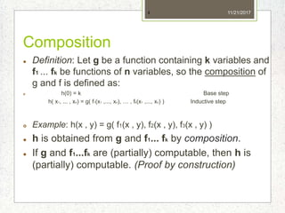
28. Unbounded minimalization
 Definition: y is the least value for which predicate P is true if it
exists. If there is no value of y for which P is true, the
unbounded minimalization is undefined.
 We can then define this as a non-total function in the
following way:
 Theorem: If P(x1, … , xn, y) is a computable predicate and if
then g is a partially computable function.
(Proof by construction)
28
min
y
P(x1,... , xn , y)
x− y= min
z
[ y+ z= x]
g(x1,. .., xn)= min
y
P(x1,. .. , xn , y)
11/21/2017

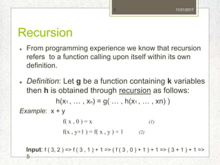
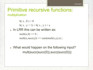
29. Additional primitive recursive
functions
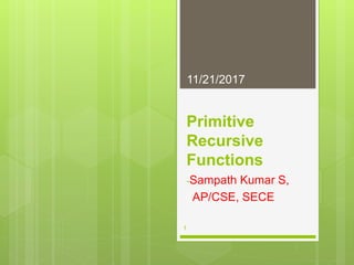
 [ x / y ] , the whole part of the division i.e. [10/4]=2
 R(x,y) , remainder of the division of x by y.
 pn , nth prime number i.e p1=2 , p2=3 etc.
29
    yxyx=yx,R /*-
    x>y+t=yx nim
xt
*1/ 
p0= 0,
pn+ 1= min
t < pn!+ 1
[Prime(t)& t> pn]
11/21/2017

30. Pairing functions
30
 Let us consider the following primitive recursive function that provides a
coding for two numbers x and y.
  1-12y2>< +=yx, x
11/21/2017

31. Pairing functions
31
 Let us consider the following primitive recursive function that provides a
coding for two numbers x and y.
Example: <1,1> = 2 * ( 2 + 1 ) ∸ 1 = 6 ∸ 1 = 5
<1,2> = 2 * ( 2*2 + 1) ∸ 1 = 10 ∸ 1 = 9
  1-12y2>< +=yx, x
11/21/2017

32. Pairing functions
32
 Let us consider the following primitive recursive function that provides a
coding for two numbers x and y.
Example: <1,1> = 2 * ( 2 + 1 ) ∸ 1 = 6 ∸ 1 = 5
<1,2> = 2 * ( 2*2 + 1) ∸ 1 = 10 ∸ 1 = 9
   12y21:012y2 +=+>yx,<followsasrearrangecanweso,+thatNote xx

  1-12y2>< +=yx, x
11/21/2017

33. Pairing functions
33
 Let us consider the following primitive recursive function that provides a
coding for two numbers x and y.
Example: <1,1> = 2 * ( 2 + 1 ) ∸ 1 = 6 ∸ 1 = 5
<1,2> = 2 * ( 2*2 + 1) ∸ 1 = 10 ∸ 1 = 9
   12y21:012y2 +=+>yx,<followsasrearrangecanweso,+thatNote xx

 Define z to be as: < x , y > = z
Then for any z there is always a unique solution x and y.
  1-12y2>< +=yx, x
11/21/2017

34. Pairing functions
34
 Let us consider the following primitive recursive function that provides a
coding for two numbers x and y.
Example: <1,1> = 2 * ( 2 + 1 ) ∸ 1 = 6 ∸ 1 = 5
<1,2> = 2 * ( 2*2 + 1) ∸ 1 = 10 ∸ 1 = 9
   12y21:012y2 +=+>yx,<followsasrearrangecanweso,+thatNote xx

 Define z to be as: < x , y > = z
Then for any z there is always a unique solution x and y.
  1212y21 +zofdivisortheisthen,+=+zthatGiven xx
  x
+z=+Then 2/112y
  1-12y2>< +=yx, x
11/21/2017

35. Pairing functions
35
 Let us consider the following primitive recursive function that provides a
coding for two numbers x and y.
Example: <1,1> = 2 * ( 2 + 1 ) ∸ 1 = 6 ∸ 1 = 5
<1,2> = 2 * ( 2*2 + 1) ∸ 1 = 10 ∸ 1 = 9
   12y21:012y2 +=+>yx,<followsasrearrangecanweso,+thatNote xx

 Define z to be as: < x , y > = z
Then for any z there is always a unique solution x and y.
  1212y21 +zofdivisortheisthen,+=+zthatGiven xx
  x
+z=+Then 2/112y
 Thus we have the solutions for x and y which can then be defined using
the following functions:  
  zzr=y
zzl=x


  1-12y2>< +=yx, x
11/21/2017

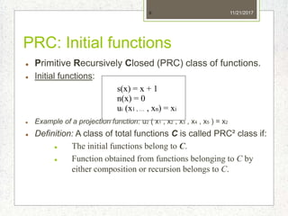
36. Pairing functions
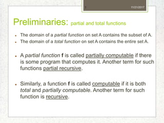
 More formally this can written as:
 Pairing Function Theorem: functions <x,y>, l(z), r(z) have
the following properties:
 are primitive recursive
 l(<x,y>) = x and r(<x,y>) = y
 < l(z) , r(z) > = z
 l(z) , r(z)≤ z
36
 
  zzr=y
zzl=x


     
     ]><[
]><[
yx,=zx=zr
yx,=zy=zl
z
nim
zy
z
nim
zx




11/21/2017

37. Gödel numbers
 Let (a1, … , an) be any sequence, then the Gödel
number is computed as follows:
37
[a1, ..., an]= ∏i= 1
n
pi
ai
11/21/2017

38. Gödel numbers
 Let (a1, … , an) be any sequence, then the Gödel
number is computed as follows:
 Example: Take a sequence (1,2,3,4), the Gödel
number will be computed as follows:
38
  4321
75321,2,3,4 =
[a1, ..., an]= ∏i= 1
n
pi
ai
11/21/2017

39. Gödel numbers
 Let (a1, … , an) be any sequence, then the Gödel
number is computed as follows:
 Example: Take a sequence (1,2,3,4), the Gödel
number will be computed as follows:
 Gödel numbering has a special uniqueness
property:
If [a1, … , an ] = [ b1, … , bn ] then
ai = bi , where i = 1, … , n
39
  4321
75321,2,3,4 =
[a1, ..., an]= ∏i= 1
n
pi
ai
11/21/2017

40. Gödel numbers
 Let (a1, … , an) be any sequence, then the Gödel
number is computed as follows:
 Example: Take a sequence (1,2,3,4), the Gödel
number will be computed as follows:
 Gödel numbering has a special uniqueness
property:
If [a1, … , an ] = [ b1, … , bn ] then
ai = bi , where i = 1, … , n
 Also notice: [ a1, … , an ] = [ a1, … , an, 0 ]
40
  4321
75321,2,3,4 =
[a1, ..., an]= ∏i= 1
n
pi
ai
11/21/2017

41. Gödel numbers
 Given that x = [a1, … , an ], we can now define two important
functions:
41
   
         00Lt
|~
1t
=xijjx=x
xp=a=x
jxi
nim
xi
i
nim
xtii
 


11/21/2017

42. Gödel numbers
 Given that x = [a1, … , an ], we can now define two important
functions:
 Example: Let x = [ 4 , 3 , 2 , 1 ], then (x)2 = 3 and (x)4=1 and (x)0 = 0
42
   
         00Lt
|~
1t
=xijjx=x
xp=a=x
jxi
nim
xi
i
nim
xtii
 


11/21/2017

43. Gödel numbers
 Given that x = [a1, … , an ], we can now define two important
functions:
 Example: Let x = [ 4 , 3 , 2 , 1 ], then (x)2 = 3 and (x)4=1 and (x)0 = 0
Lt(10) = will be the length of the sequence derived using Gödel
numbering
43
   
         00Lt
|~
1t
=xijjx=x
xp=a=x
jxi
nim
xi
i
nim
xtii
 


11/21/2017

44. Gödel numbers
 Given that x = [a1, … , an ], we can now define two important
functions:
 Example: Let x = [ 4 , 3 , 2 , 1 ], then (x)2 = 3 and (x)4=1 and (x)0 = 0
Lt(10) = will be the length of the sequence derived using Gödel
numbering
So: 10 = 2^1 * 3^0 * 5^1 = [ 1, 0, 1 ] => Lt(10) = 3
44
   
         00Lt
|~
1t
=xijjx=x
xp=a=x
jxi
nim
xi
i
nim
xtii
 


11/21/2017

45. Gödel numbers
 Given that x = [a1, … , an ], we can now define two important
functions:
 Example: Let x = [ 4 , 3 , 2 , 1 ], then (x)2 = 3 and (x)4=1 and (x)0 = 0
Lt(10) = will be the length of the sequence derived using Gödel
numbering
So: 10 = 2^1 * 3^0 * 5^1 = [ 1, 0, 1 ] => Lt(10) = 3
 Sequence Number Theorem:
45
  





 
otherwise
niifa
=a,a i
n
0
1
...1,
(1)
   
         00Lt
|~
1t
=xijjx=x
xp=a=x
jxi
nim
xi
i
nim
xtii
 


11/21/2017

46. Gödel numbers
 Given that x = [a1, … , an ], we can now define two important
functions:
 Example: Let x = [ 4 , 3 , 2 , 1 ], then (x)2 = 3 and (x)4=1 and (x)0 = 0
Lt(10) = will be the length of the sequence derived using Gödel
numbering
So: 10 = 2^1 * 3^0 * 5^1 = [ 1, 0, 1 ] => Lt(10) = 3
 Sequence Number Theorem:
46
  





 
otherwise
niifa
=a,a i
n
0
1
...1,
(1)
(2)       xnifx=x,x n Lt...1, 
   
         00Lt
|~
1t
=xijjx=x
xp=a=x
jxi
nim
xi
i
nim
xtii
 


11/21/2017