Applied Econometrics
Autocorrelation
1. Whatis autocorrelation
2. What causes autocorrelation
3. First and higher orders
4. Consequences of autocorrelation
5. Detecting autocorrelation
6. Resolving autocorrelation
3.
Applied Econometrics
Learning Objectives
1.Understand meaning of autocorrelation in the CLRM
2. What causes autocorrelation
3. Distinguish among first and higher orders of autocorrelation
4. Understand consequences of autocorrelation on OLS
estimates
5. Detect autocorrelation through graph inspection
6. Detect autocorrelation through formal econometric tests
7. Perform autocorrelation tests using econometric software
8. Resolve autocorrelation using econometric software
4.
Applied Econometrics
What isAutocorrelation
There should be no co-variance /correlation
among the disturbance term of two different
time periods. Assumption 6 of the CLRM
states that the covariances and correlations
between different disturbances are all zero:
cov(ut, us)=0
This assumption states that the disturbances ut
and us are independently distributed, which is
called serial independence
What is Autocorrelation
5.
Applied Econometrics
If thisassumption is no longer valid, then the
disturbances are not independent, but pairwise
autocorrelated (or serially correlated).
This means that an error occurring at period t may
be carried over to the next period t+1.
Autocorrelation most likely to occur in time series
data.
In cross-sectional we can change the arrangement
of the data without altering the results.
What is Autocorrelation (2)
6.
Applied Econometrics
One factorthat can cause autocorrelation is
omitted variables.
Suppose Yt is related to X2t and X3t, but we
wrongfully do not include X3t in our model.
It means if you exclude the important
determinant (Independent variable) of
dependent variable.
What Causes Autocorrelation
7.
Applied Econometrics
Another possiblereason is misspecification.
Suppose Yt is related to X2t with a quadratic
relationship:
Yt=β1+β2X2
2t+ut
but we wrongfully assume and estimate a
straight line:
Yt=β1+β2X2t+ut
Then the error term obtained from the straight
line will depend on X2
2t.
What Causes Autocorrelation (2)
8.
Applied Econometrics
A thirdreason is systematic errors in
measurement.
Suppose a company updates its inventory at a
given period in time.
If a systematic error occurred then the
cumulative inventory stock will exhibit
accumulated measurement errors.
These errors will show up as an autocorrelated
procedure.
What Causes Autocorrelation (3)
9.
Applied Econometrics
order ofAutocorrelation
The simplest and most commonly observed is the
first-order autocorrelation.
If the residual is depending on its one previous
value that is called 1st
order autocorrelation. We
can name it AR(1)
First-order Autocorrelation
10.
Applied Econometrics
The coefficientρ is called the first-order
autocorrelation coefficient and takes values
from -1 to +1.
It is obvious that the size of ρ will determine
the strength of serial correlation.
There can be three different cases.
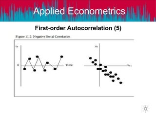
First-order Autocorrelation (2)
11.
Applied Econometrics
(a) Ifρ is zero, then we have no autocorrelation.
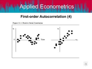
(b) If ρ approaches unity, the value of the
previous observation of the error becomes
more important in determining the value of the
current error and therefore high degree of
autocorrelation exists. In this case we have
positive autocorrelation.
(c) If ρ approaches -1, we have high degree of
negative autocorrelation.
First-order Autocorrelation (3)
Applied Econometrics
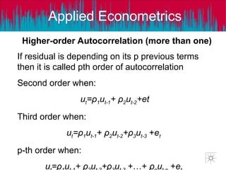
Higher-order Autocorrelation(more than one)
If residual is depending on its p previous terms
then it is called pth order of autocorrelation
Second order when:
ut=ρ1ut-1+ ρ2ut-2+et
Third order when:
ut=ρ1ut-1+ ρ2ut-2+ρ3ut-3 +et
p-th order when:
u =ρ u + ρ u +ρ u +…+ ρ u +e
15.
Applied Econometrics
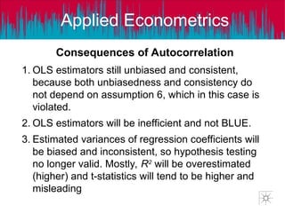
Consequences ofAutocorrelation
1. OLS estimators still unbiased and consistent,
because both unbiasedness and consistency do
not depend on assumption 6, which in this case is
violated.
2. OLS estimators will be inefficient and not BLUE.
3. Estimated variances of regression coefficients will
be biased and inconsistent, so hypothesis testing
no longer valid. Mostly, R2
will be overestimated
(higher) and t-statistics will tend to be higher and
misleading
16.
Applied Econometrics
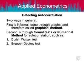
Detecting Autocorrelation
Twoways in general.
First is informal, done through graphs, and
therefore called graphical method.
Second is through formal tests or Numerical
Method for autocorrelation, such as:
1. Durbin Watson test
2. Breusch-Godfrey test
17.
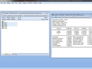
Applied Econometrics
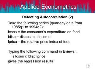
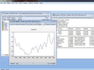
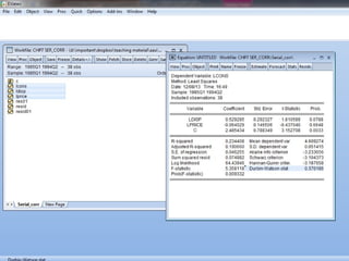
Take thefollowing series (quarterly data from
1985q1 to 1994q2):
lcons = the consumer’s expenditure on food
ldisp = disposable income
lprice = the relative price index of food
Typing the following command in Eviews :
ls lcons c ldisp lprice
gives the regression results
Detecting Autocorrelation (2)
18.
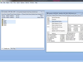
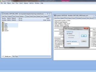
Applied Econometrics
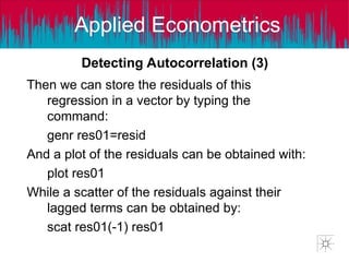
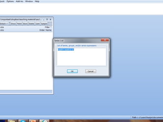
Then wecan store the residuals of this
regression in a vector by typing the
command:
genr res01=resid
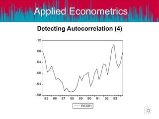
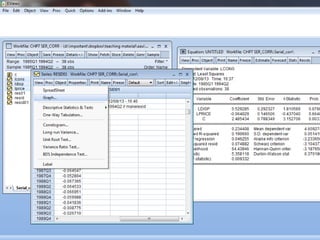
And a plot of the residuals can be obtained with:
plot res01
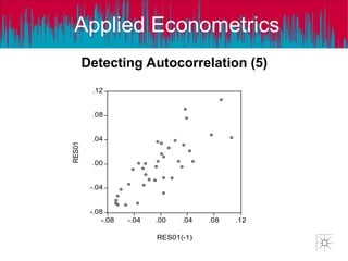
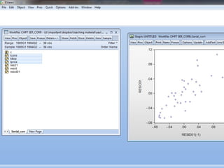
While a scatter of the residuals against their
lagged terms can be obtained by:
scat res01(-1) res01
Detecting Autocorrelation (3)
Applied Econometrics
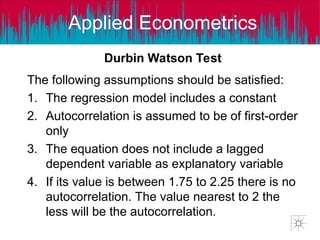
Durbin WatsonTest
The following assumptions should be satisfied:
1. The regression model includes a constant
2. Autocorrelation is assumed to be of first-order
only
3. The equation does not include a lagged
dependent variable as explanatory variable
4. If its value is between 1.75 to 2.25 there is no
autocorrelation. The value nearest to 2 the
less will be the autocorrelation.
29.
Applied Econometrics
Step 1:Estimate model by OLS and obtain the
residuals
Step 2: Calculate DW statistic
Step 3: Conclude
Durbin Watson Test (2)
30.
Applied Econometrics
Drawbacks ofthe DW test:
1.May give inconclusive results
2.Not applicable when a lagged dependent
variable is used
3.Can’t take into account higher order of
autocorrelation
Durbin Watson Test (4)
Applied Econometrics
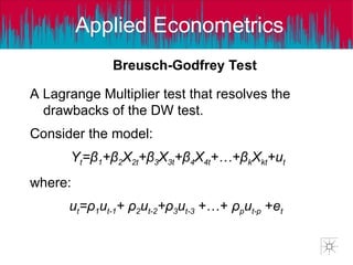
Breusch-Godfrey Test
ALagrange Multiplier test that resolves the
drawbacks of the DW test.
Consider the model:
Yt=β1+β2X2t+β3X3t+β4X4t+…+βkXkt+ut
where:
ut=ρ1ut-1+ ρ2ut-2+ρ3ut-3 +…+ ρput-p +et
33.
Applied Econometrics
It isa general test for at any order
autocorrelation could be tested. F & p-
values are the decision criterias of
autocorrelation.
Ho= There is no autocorrelation
H1= There is autocorrelation
Breusch-Godfrey Test (2)
34.
Applied Econometrics
Step 1:Estimate model and obtain the residuals
Step 2: Run full LM model with the number of
lags used being determined by the assumed
order of autocorrelation
Step 3: Conclude
Breusch-Godfrey Test (3)
Applied Econometrics
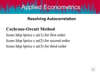
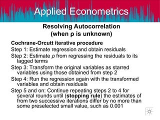
Resolving Autocorrelation
(whenρ is unknown)
Cochrane-Orcutt iterative procedure
Step 1: Estimate regression and obtain residuals
Step 2: Estimate ρ from regressing the residuals to its
lagged terms
Step 3: Transform the original variables as starred
variables using those obtained from step 2
Step 4: Run the regression again with the transformed
variables and obtain residuals
Step 5 and on: Continue repeating steps 2 to 4 for
several rounds until (stopping rule) the estimates of
from two successive iterations differ by no more than
some preselected small value, such as 0.001