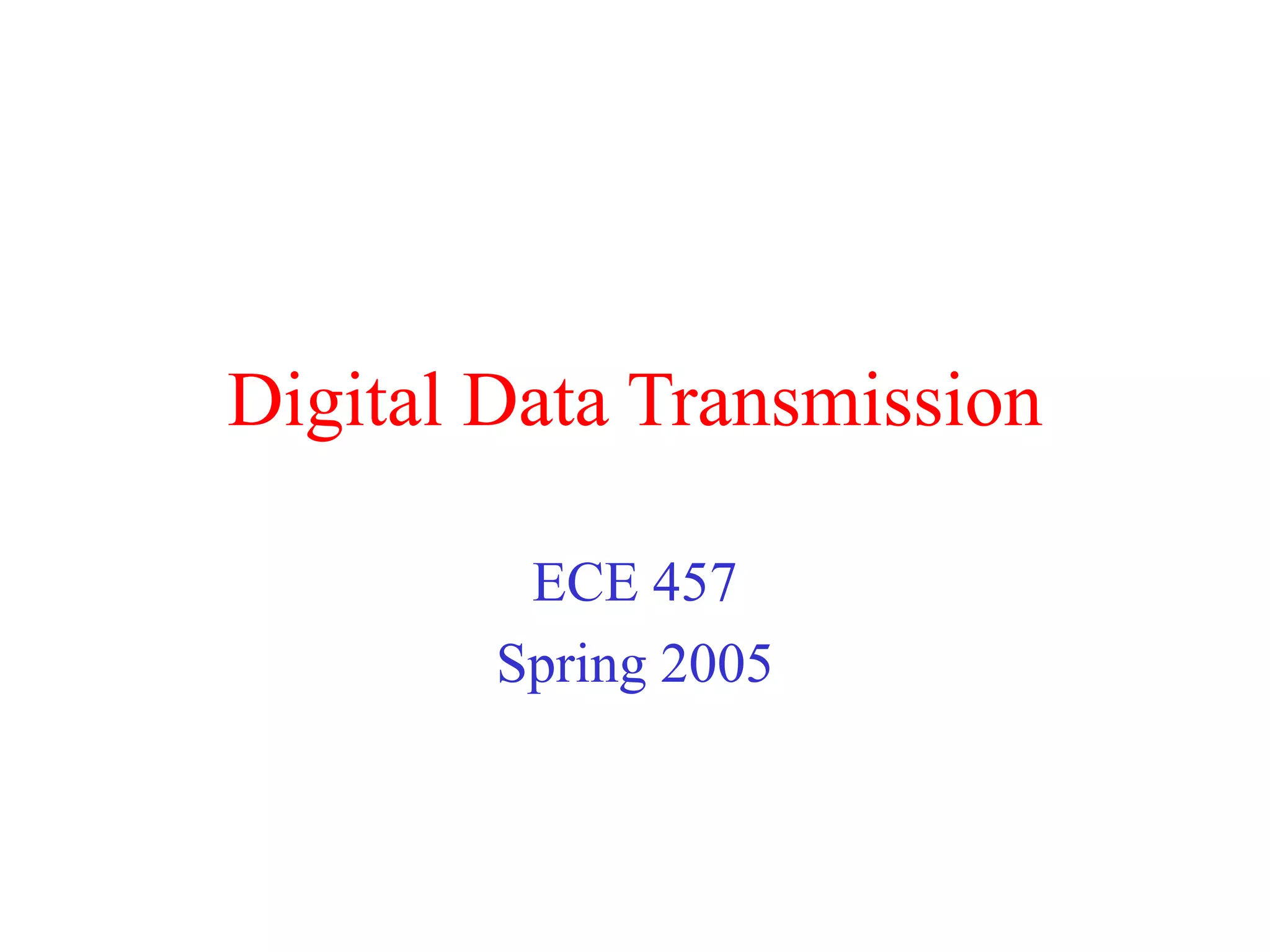
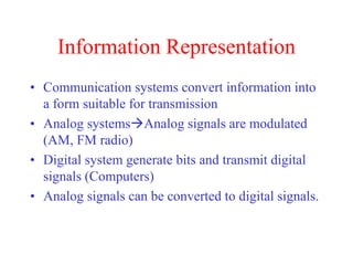
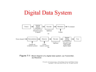
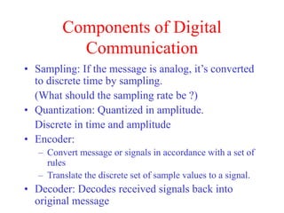
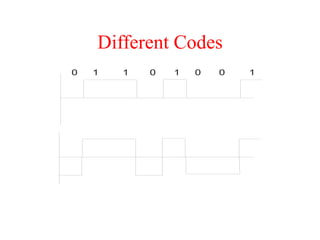
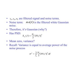
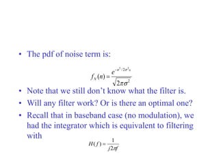
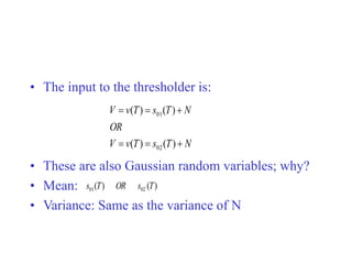
This document discusses digital data transmission and communication systems. It begins by comparing analog and digital signals, noting that digital signals have discrete values while analog signals are continuous. The key components of digital communication systems are then introduced, including sampling, quantization, encoding, and decoding. Different coding techniques like ASK, PSK, and FSK are also described. The document concludes by analyzing the performance of digital communication systems using metrics like data rate, bit error rate, and probability of error as a function of signal-to-noise ratio.
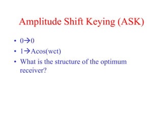
![Receiver Preformance
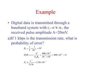
• The output of the integrator:
• is a random variable.
• N is Gaussian. Why?
sent
is
A
N
AT
sent
is
A
N
AT
dt
t
n
t
s
V
T
t
t
0
0
)]
(
)
(
[
T
t
t
dt
t
n
N
0
0
)
(](https://image.slidesharecdn.com/digitaldatatransmission-221127142749-ff09b081/85/Digital-Data-Transmission-ppt-13-320.jpg)
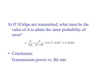
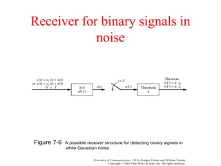
![Analysis
• Key Point
– White noise is uncorrelated
2
)
!
?(
)
(
2
)]
(
)
(
[
)
(
?
]
[
]
[
]
[
]
[
0
)]
(
[
]
)
(
[
]
[
0
0
2
2
2
2
0
0
0
0
0
0
0
0
0
0
0
0
0
0
T
N
ed
uncorrelat
is
noise
White
Why
dtds
s
t
N
dtds
s
n
t
n
E
dt
t
n
E
Why
N
E
N
E
N
E
N
Var
dt
t
n
E
dt
t
n
E
N
E
T
t
t
T
t
t
T
t
t
T
t
t
T
t
t
T
t
t
T
t
t
](https://image.slidesharecdn.com/digitaldatatransmission-221127142749-ff09b081/85/Digital-Data-Transmission-ppt-14-320.jpg)
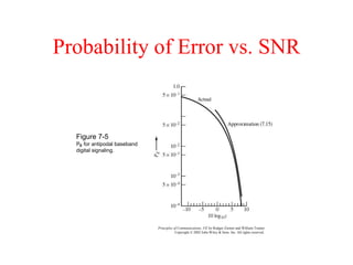
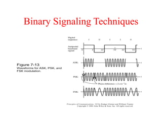
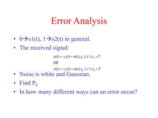
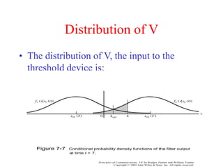
![Probability of Error
• Two types of errors:
• The average probability of error:
)
(
1
2
))
(
|
(
)
(
2
))
(
|
(
02
2
2
/
)]
(
[
2
01
2
2
/
)]
(
[
1
2
2
02
2
2
01
T
s
k
Q
dv
e
t
s
E
P
T
s
k
Q
dv
e
t
s
E
P
k T
s
v
k
T
s
v
)]
(
|
[
2
1
)]
(
|
[
2
1
2
1 t
s
E
P
t
s
E
P
PE
](https://image.slidesharecdn.com/digitaldatatransmission-221127142749-ff09b081/85/Digital-Data-Transmission-ppt-34-320.jpg)
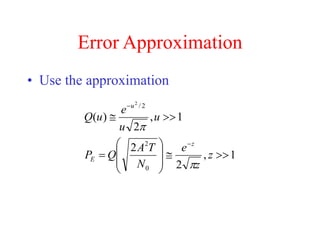
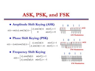
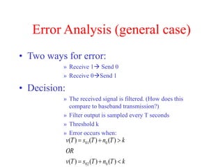
![• Goal: Minimize the average probability of
errror
• Choose the optimal threshold
• What should the optimal threshold, kopt be?
• Kopt=0.5[s01(T)+s02(T)]
•
2
)
(
)
( 01
02 T
s
T
s
Q
PE](https://image.slidesharecdn.com/digitaldatatransmission-221127142749-ff09b081/85/Digital-Data-Transmission-ppt-35-320.jpg)