Downloaded 22 times

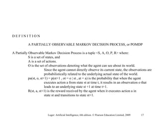
![function Viterbi(Observations of length T, Probabilistic FSM)
begin
number := number of states in FSM
create probability matrix viterbi[R = N + 2, C = T + 2];
viterbi[0, 0] := 1.0;
for each time step (observation) t from 0 to T do
for each state si from i = 0 to number do
for each transition from si to sj in the Probabilistic FSM do
begin
new-count := viterbi[si, t] x path[si, sj] x p(sj | si);
if ((viterbi[sj, t + 1] = 0) or (new-count > viterbi[sj, t + 1]))
then
begin
viterbi[si, t + 1] := new-count
append back-pointer [sj , t + 1] to back-pointer list
end
end;
return viterbi[R, C];
return back-pointer list
end.
Luger: Artificial Intelligence, 6th edition. © Pearson Education Limited, 2009 11](https://image.slidesharecdn.com/sixthedchap13-170228102732/85/Artificial-Intelligence-11-320.jpg)

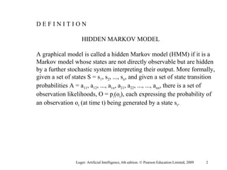
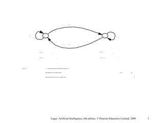
This document discusses probabilistic machine learning models including hidden Markov models, dynamic Bayesian networks, and reinforcement learning. It provides definitions and examples of these concepts. Hidden Markov models are graphical models where the states are hidden and represented by observable outputs. Dynamic Bayesian networks are Bayesian networks that model systems changing over time. Reinforcement learning models sequential decision making problems where an agent takes actions in an environment to maximize rewards.