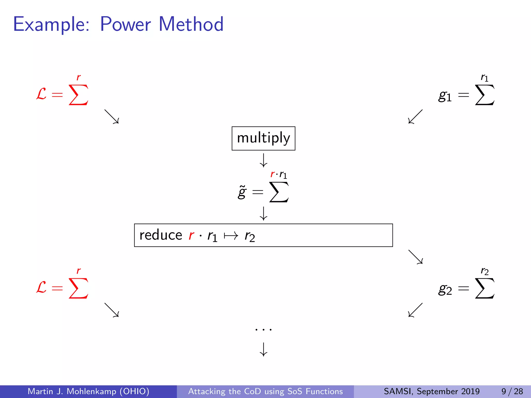
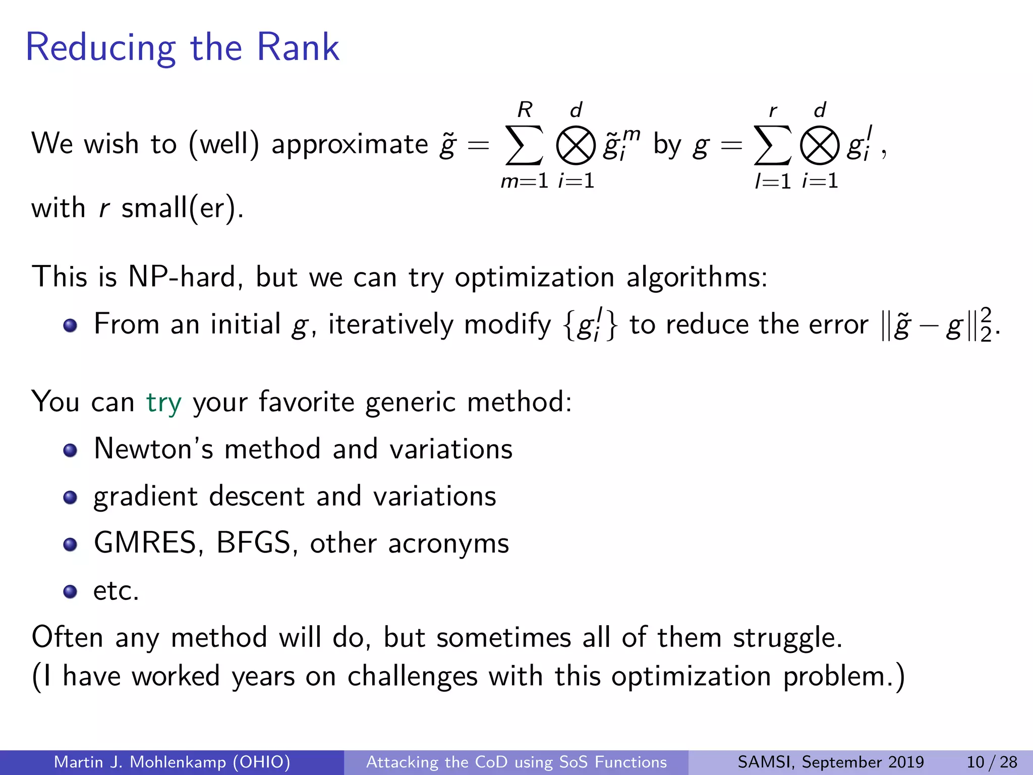
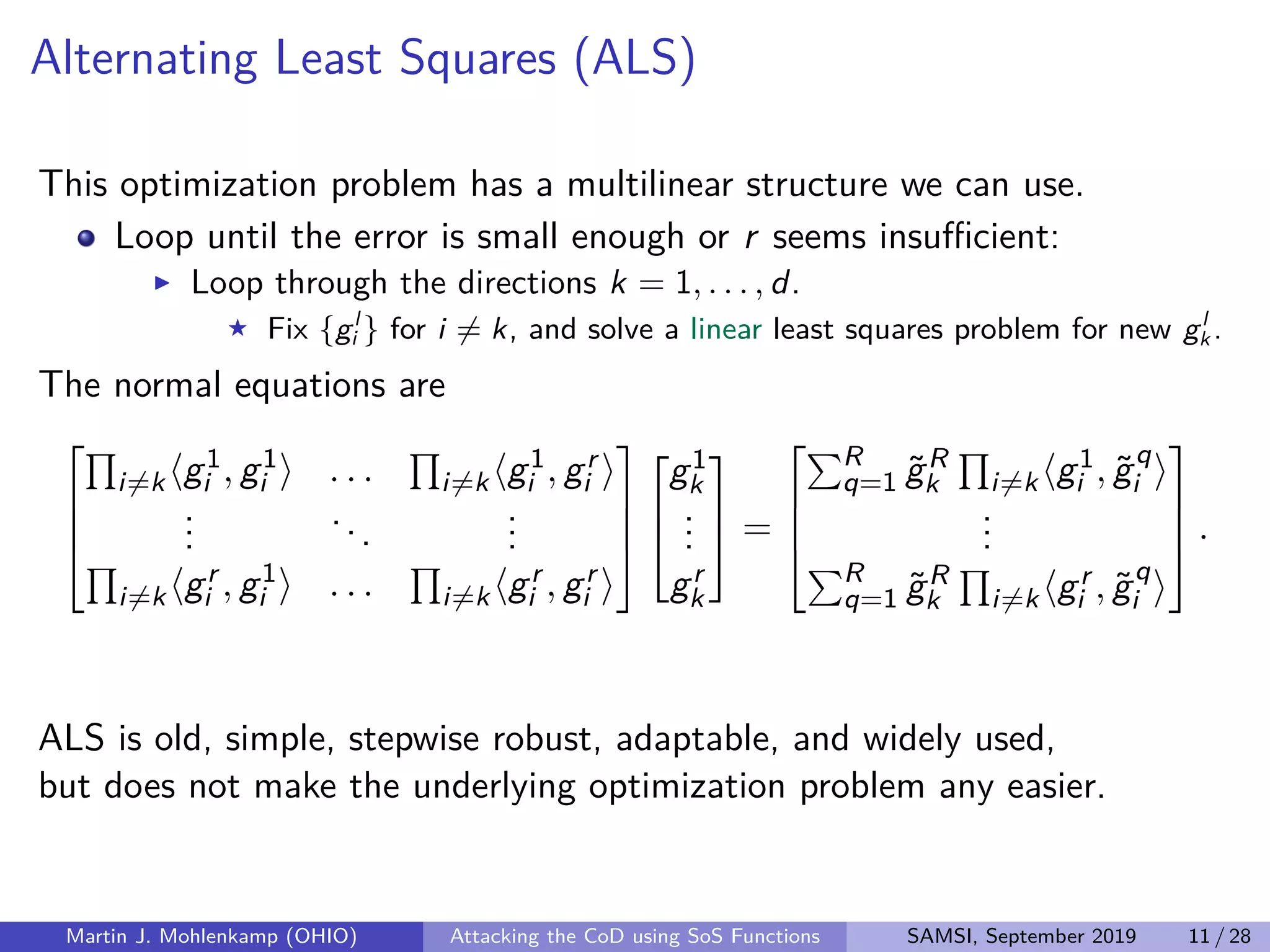
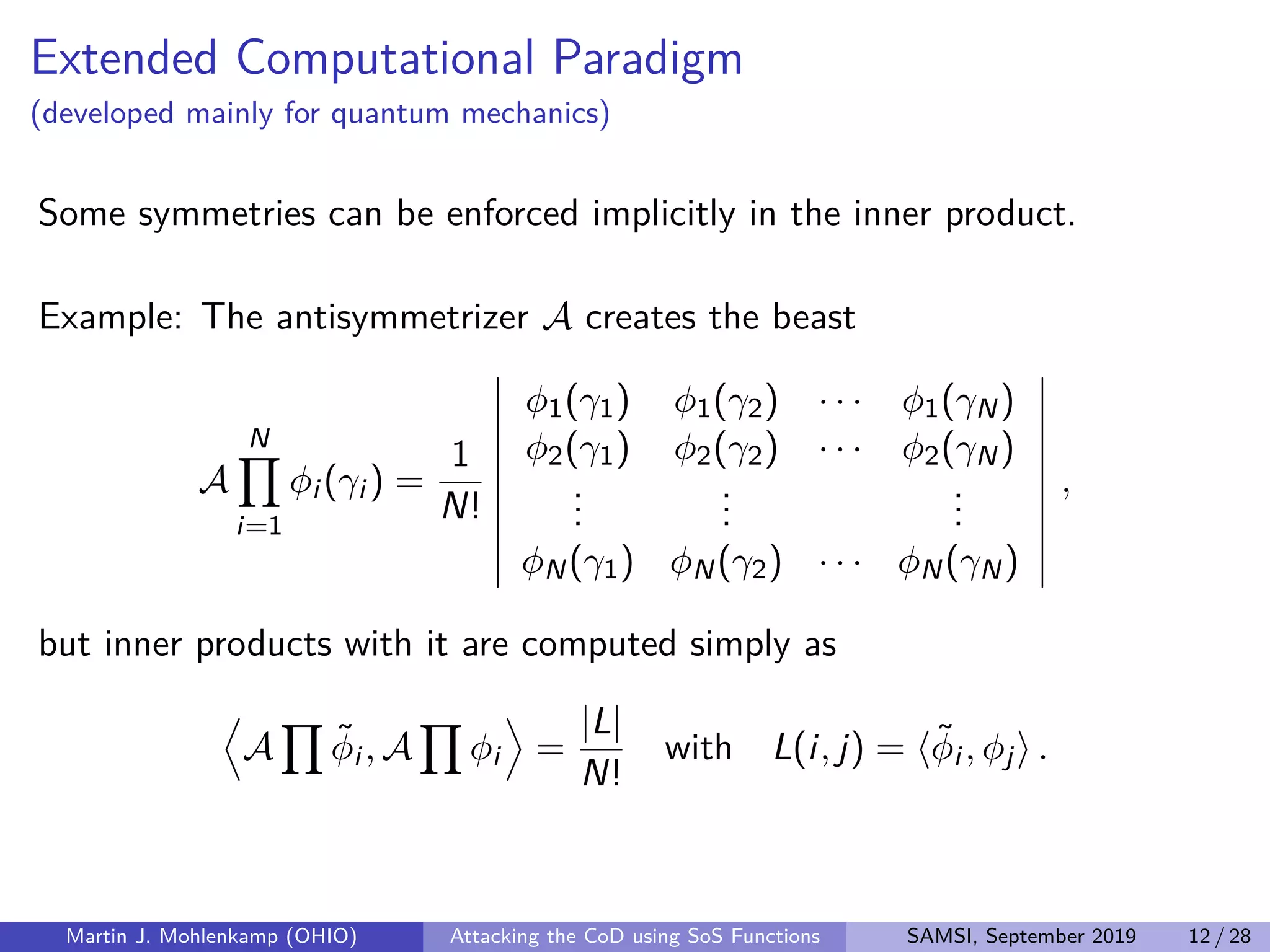
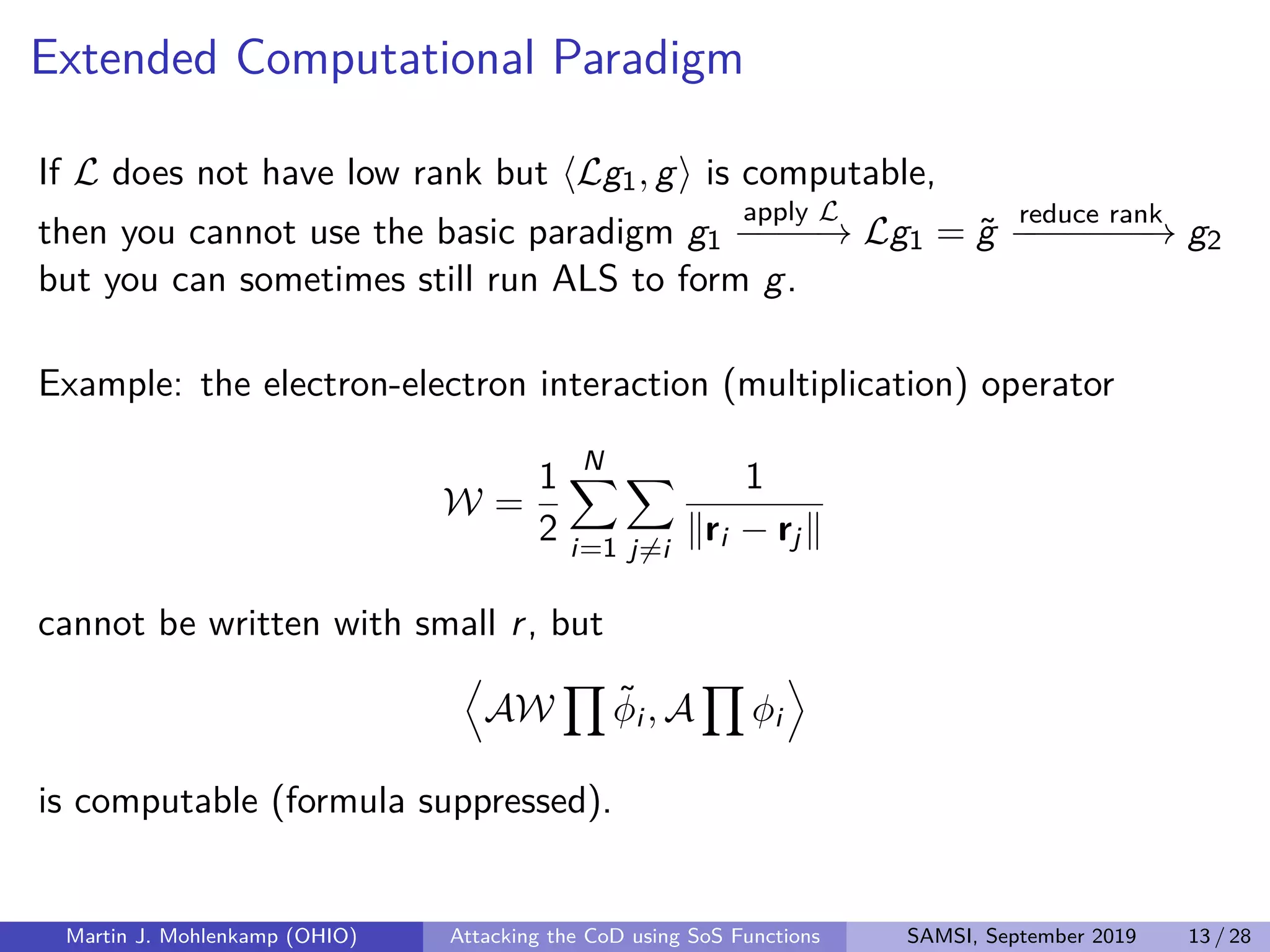
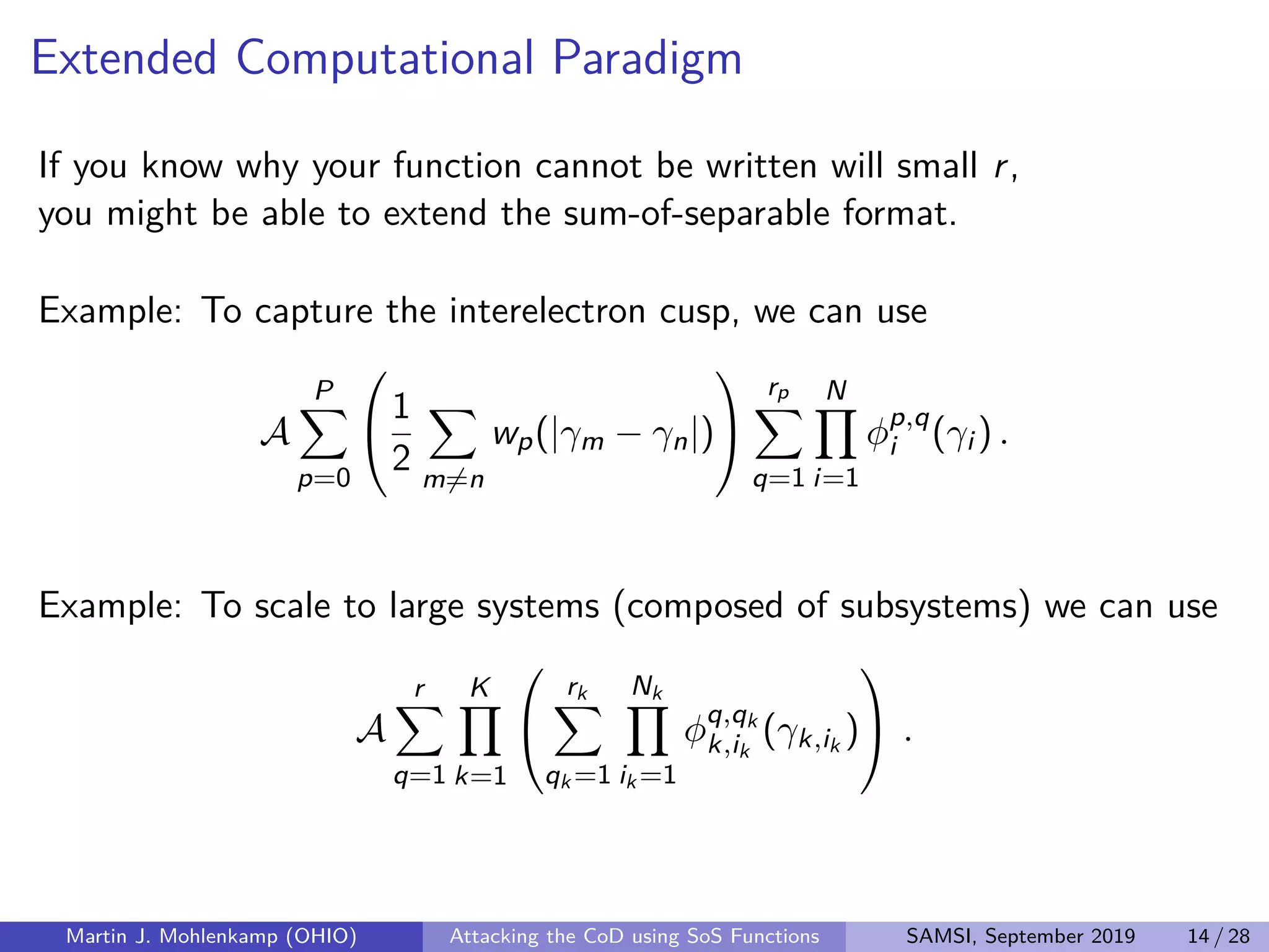
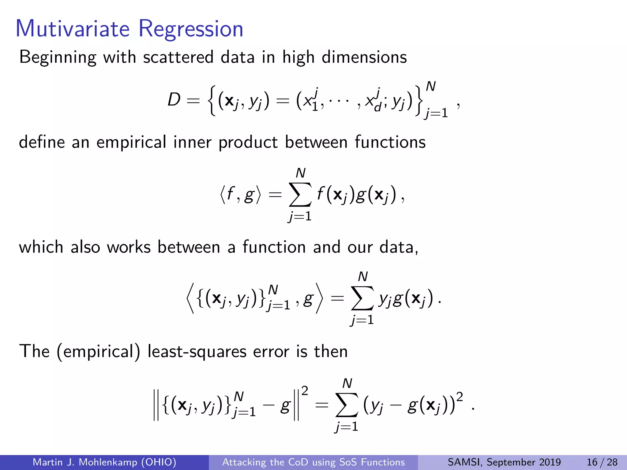
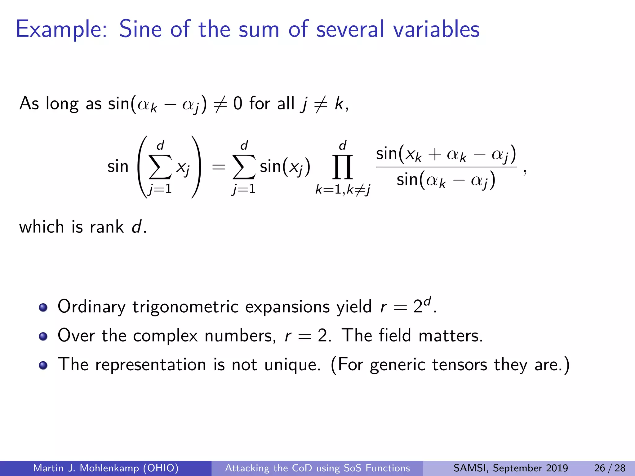
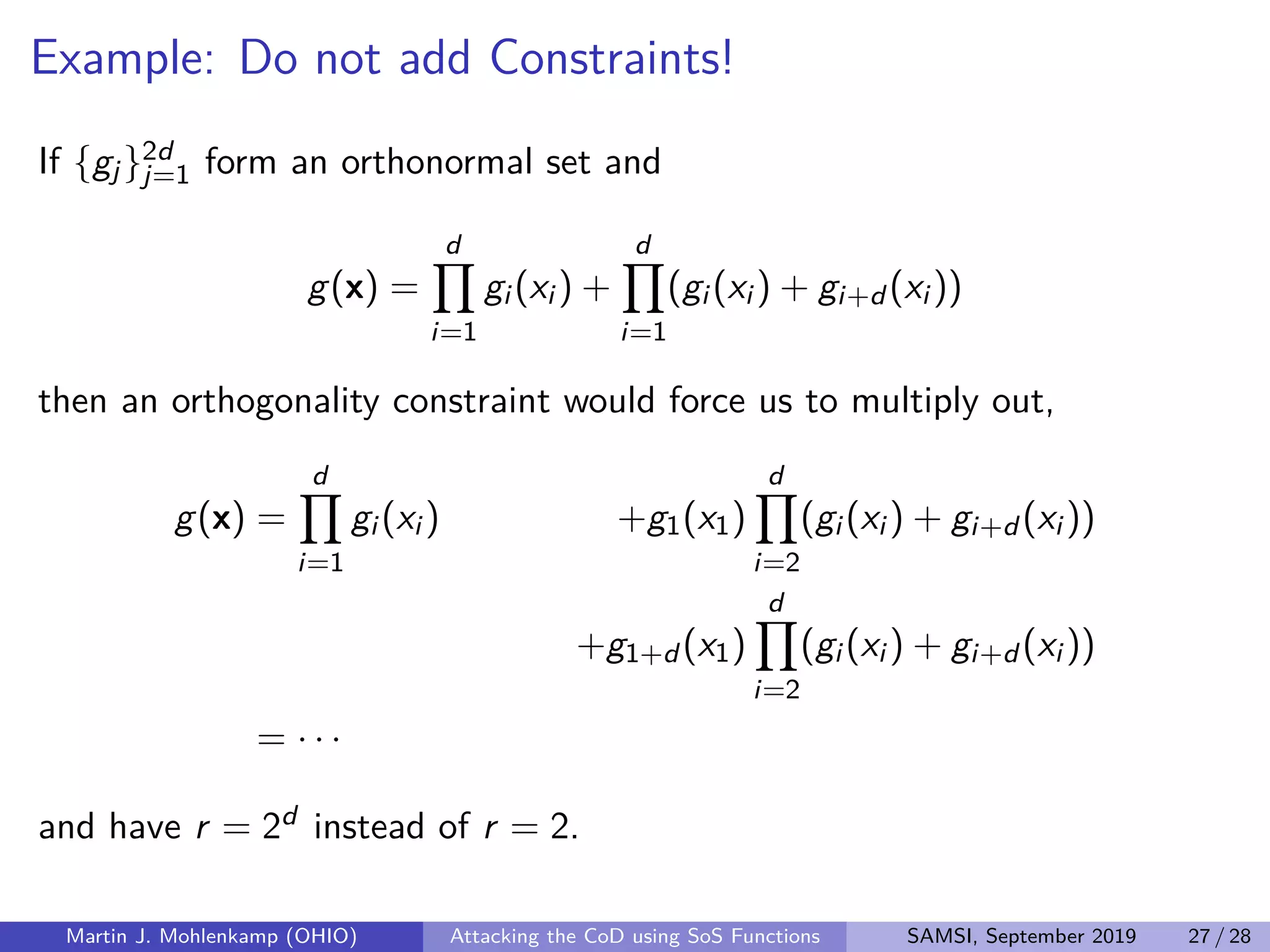
Download as PDF, PPTX
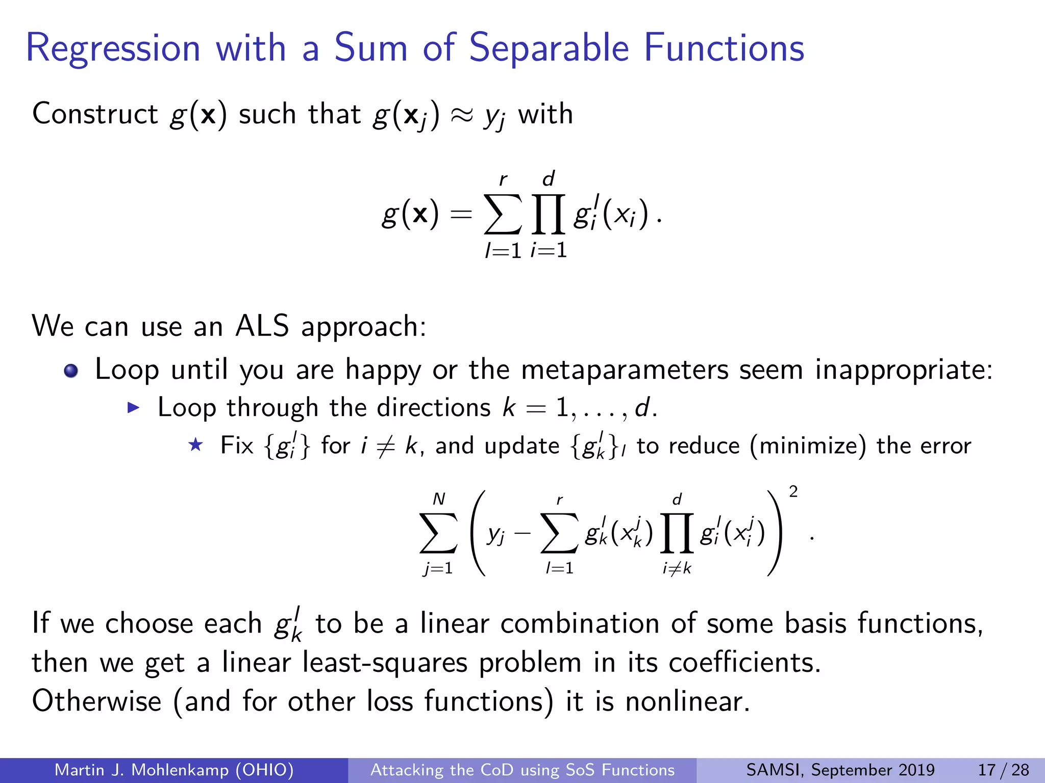
![Regression with Consistent Functions
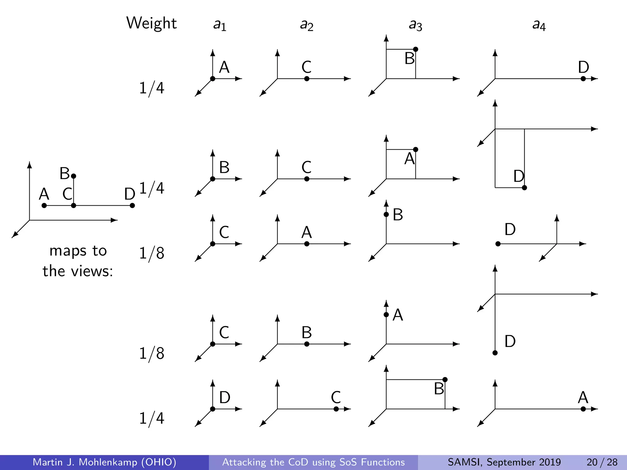
From a function g on ordered lists of atoms, we can build a function on
structures that is rotation and translation invariant by defining
Cg(σ) =
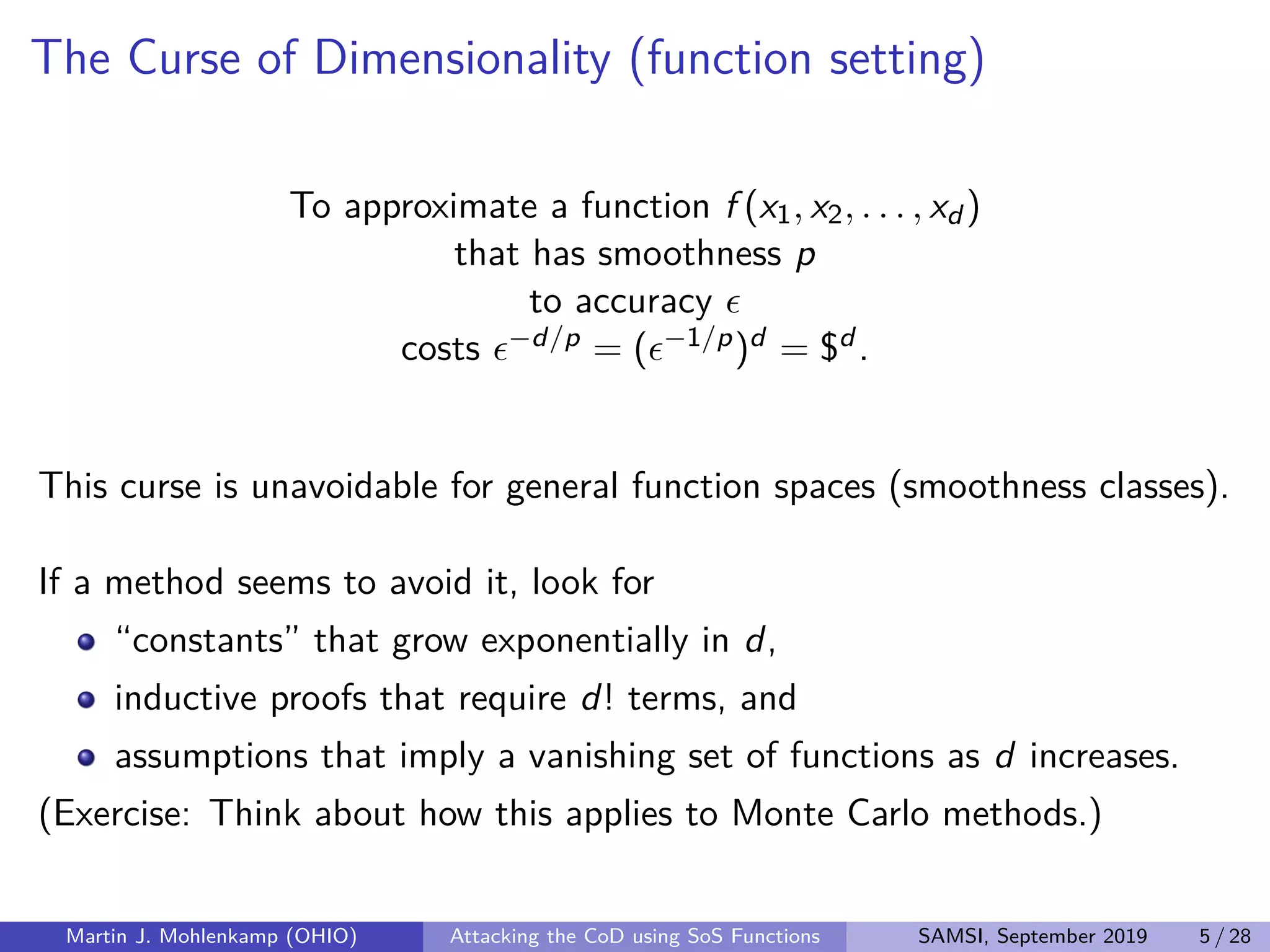
(w,v)∈Vσ
wg(v) .
We can then attempt to minimize the least-squares error
D −Cg 2
=
1
N
N
j=1
(yj − Cg(σj))2
=
1
N
N
j=1
yj −
(w,v)∈Vσj
wg(v)
2
.
If g([a1, a2, . . .]) := g([a1, a2, . . . , ad ]) =
r
l=1
d
i=1
gl
i (ai ) ,
then ALS can be run. Each gl
i is a function of a = (t, r), so its domain is
several copies of R3, which is tractable.
Martin J. Mohlenkamp (OHIO) Attacking the CoD using SoS Functions SAMSI, September 2019 21 / 28](https://image.slidesharecdn.com/mohlenkampseminar-190924151208/75/2019-Fall-Series-Postdoc-Seminars-Special-Guest-Lecture-Attacking-the-Curse-of-Dimensionality-Using-Sums-of-Separable-Functions-Martin-Mohlenkamp-September-11-2019-21-2048.jpg)

The document discusses strategies for addressing the curse of dimensionality in high-dimensional functions by approximating them as sums of separable functions or tensors. It outlines the computational benefits of this approach in numerical analysis and machine learning, particularly through methods like alternating least squares and regression techniques. The author emphasizes the utility of these methods while also acknowledging ongoing challenges and potential limitations.