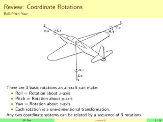
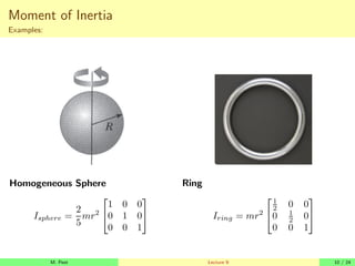
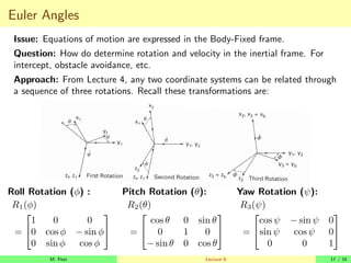
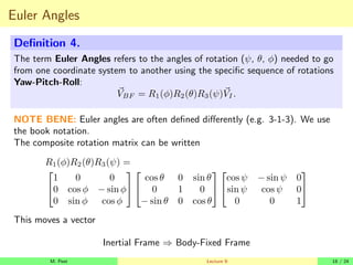
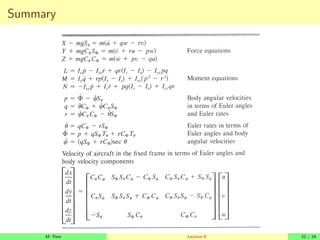
This lecture covers the 6 degree-of-freedom equations of motion for spacecraft and aircraft. It begins with a review of Newton's laws, rotating reference frames, and coordinate rotations. It then derives the equations of motion for linear and angular momentum in an inertial frame and body-fixed frame. Due to the body-fixed frame rotating, additional terms are needed in the equations of motion. Euler angles are also introduced to relate vectors between the inertial and body-fixed frames.
![6DOF: Newton’s Laws
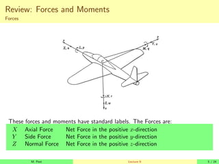
Forces
Newton’s Second Law tells us that for a particle F = ma. In vector form:
~
F =
X
i
~
Fi = m
d
dt
~
V
That is, if ~
F = [Fx Fy Fz] and ~
V = [u v w], then
Fx = m
du
dt
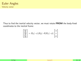
Fx = m
dv
dt
Fz = m
dw
dt
Definition 1.
~
L = m~
V is referred to as Linear Momentum.
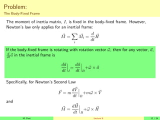
Newton’s Second Law is only valid if ~
F and ~
V are defined in an Inertial
coordinate system.
Definition 2.
A coordinate system is Inertial if it is not accelerating or rotating.
M. Peet Lecture 9: 7 / 24](https://image.slidesharecdn.com/6dof-231105070429-292d786d/85/6-dof-pdf-7-320.jpg)
![Newton’s Laws
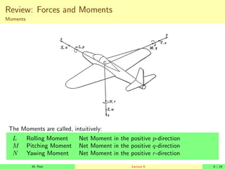
Moments
Using Calculus, this concept can be extended to rigid bodies by integration over
all particles.
~
M =
X
i
~
Mi =
d
dt
~
H
Definition 3.
Where ~
H =
R
(~
rc × ~
vc)dm is the angular momentum.
Angular momentum of a rigid body can be found as
~
H = I~
ωI
where ~
ωI = [p, q, r]T
is the angular rotation vector of the body about the
center of mass.
• p is rotation about the x-axis.
• q is rotation about the y-axis.
• r is rotation about the z-axis.
• ωI is defined in an Inertial Frame.
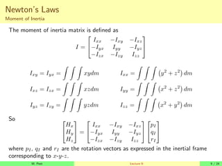
The matrix I is the Moment of Inertia Matrix.
M. Peet Lecture 9: 8 / 24](https://image.slidesharecdn.com/6dof-231105070429-292d786d/85/6-dof-pdf-8-320.jpg)


![[Deck] What's New in Spark-Iceberg Integration via DSV2.pptx](https://cdn.slidesharecdn.com/ss_thumbnails/deckwhatsnewinspark-icebergintegrationviadsv2-260210005337-25955b12-thumbnail.jpg?width=640&height=640&fit=bounds)


