Probability
• Probability isa method for measuring and quantifying the likelihood of obtaining a
specific sample from a specific population.
• We define probability as a fraction or a proportion.
• The probability of any specific outcome is determined by a ratio comparing the
frequency of occurrence for that outcome relative to the total number of possible
outcomes.
4.
Probability (cont.)
• Probabilityis determined by a fraction or proportion.
• When a population of scores is represented by a frequency distribution, probabilities
can be defined by proportions of the distribution.
• In graphs, probability can be defined as a proportion of area under the curve.
5.
5
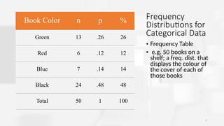
Frequency
Distributions for
Categorical Data
•Frequency Table
• e.g. 50 books on a
shelf; a freq. dist. that
displays the colour of
the cover of each of
those books
Book Color n p %
Green 13 .26 26
Red 6 .12 12
Blue 7 .14 14
Black 24 .48 48
Total 50 1 100
6.
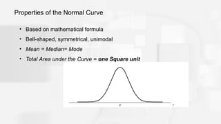
Properties of theNormal Curve
• Based on mathematical formula
• Bell-shaped, symmetrical, unimodal
• Mean = Median= Mode
• Total Area under the Curve = one Square unit
7.
7
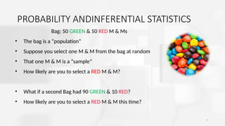
PROBABILITY ANDINFERENTIAL STATISTICS
Bag:50 GREEN & 50 RED M & Ms
• The bag is a “population”
• Suppose you select one M & M from the bag at random
• That one M & M is a “sample”
• How likely are you to select a RED M & M?
• What if a second Bag had 90 GREEN & 10 RED?
• How likely are you to select a RED M & M this time?
8.
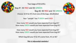
Two bags ofM & M’s:
Bag #1: 50 RED and 50 GREEN
Bag #2: 90 RED and 10 GREEN
Choose 10 M & M’s from one of the bags, blindfolded
Your “sample” has 7 GREEN and 3 RED
How many RED would you have expected from bag #1?
How many GREEN would you have expected from bag #1?
How many RED would you have expected from bag #2?
How many GREEN would you have expected from bag #2?
Which bag did your M & M’s come from, #1 or #2?
This is inferential statistics!
9.
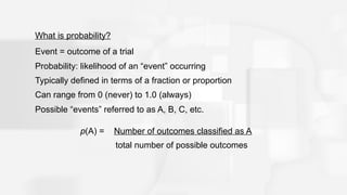
What is probability?
Event= outcome of a trial
Probability: likelihood of an “event” occurring
Typically defined in terms of a fraction or proportion
Can range from 0 (never) to 1.0 (always)
Possible “events” referred to as A, B, C, etc.
p(A) = Number of outcomes classified as A
total number of possible outcomes
10.
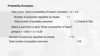
Probability Examples:
Toss acoin, what is probability of heads? p(heads) = ½ = 0.5
Number of outcomes classified as Heads = 1
Total number of possible outcomes = 2 (Head & Tail)
Select a card from a deck. What is probability of Heart?
p(Heart) = 13/52 = ¼ = 0.25
Number of outcomes classified as Hearts = 13
Total number of possible outcomes = 52
11.
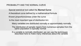
PROBABILITY AND THENORMAL CURVE
Special statistical tool called the Normal Curve
A theoretical curve defined by a mathematical formula
Known proportions/areas under the curve
Is the most important type of distribution b/c:
Many variables are distributed normally or approximately normally
The distribution of sample means from numerous samples from the
same population is typically normal
If a variable is normally distributed, we can use the techniques
described here to make many inferences about the variable
12.
Properties of theNormal Curve
• Based on mathematical formula
• Bell-shaped, symmetrical, unimodal
• Mean = Median= Mode
• Total Area under the Curve = one Square unit
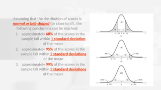
Assuming that thedistribution of scores is
normal or bell-shaped (or close to it!), the
following conclusions can be reached:
1. approximately 68% of the scores in the
sample fall within 1 standard deviation
of the mean
2. approximately 95% of the scores in the
sample fall within 2 standard deviations
of the mean
3. approximately 99% of the scores in the
sample fall within 3 standard deviations
of the mean
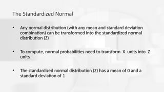
The Standardized Normal
•Any normal distribution (with any mean and standard deviation
combination) can be transformed into the standardized normal
distribution (Z)
• To compute, normal probabilities need to transform X units into Z
units
• The standardized normal distribution (Z) has a mean of 0 and a
standard deviation of 1
17.
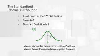
The Standardized
Normal Distribution
•Also known as the “Z” distribution
• Mean is 0
• Standard Deviation is 1
Z
f(Z)
0
1
Values above the mean have positive Z-values.
Values below the mean have negative Z-values.
18.
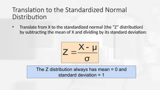
Translation to theStandardized Normal
Distribution
• Translate from X to the standardized normal (the “Z” distribution)
by subtracting the mean of X and dividing by its standard deviation:
σ
μ
X
Z
The Z distribution always has mean = 0 and
standard deviation = 1
19.
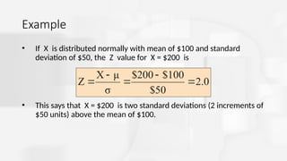
Example
• If Xis distributed normally with mean of $100 and standard
deviation of $50, the Z value for X = $200 is
• This says that X = $200 is two standard deviations (2 increments of
$50 units) above the mean of $100.
2.0
$50
100
$
$200
σ
μ
X
Z
20.
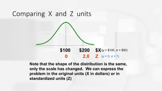
Comparing X andZ units
Note that the shape of the distribution is the same,
only the scale has changed. We can express the
problem in the original units (X in dollars) or in
standardized units (Z)
Z
$100
2.0
0
$200 $X(μ = $100, σ = $50)
(μ = 0, σ = 1)
21.
Probability is measuredby the area under
the curve
a b X
f(X)
P a X b
( )
≤
≤
P a X b
( )
<
<
=
(Note that the probability
of any individual value is
zero)
Finding Normal Probabilities
22.
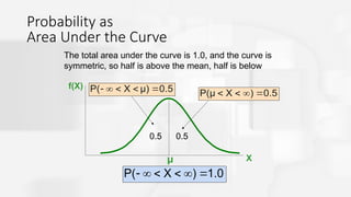
Probability as
Area Underthe Curve
The total area under the curve is 1.0, and the curve is
symmetric, so half is above the mean, half is below
f(X)
X
μ
0.5
0.5
1.0
)
X
P(
0.5
)
X
P(μ
0.5
μ)
X
P(
23.
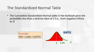
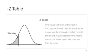
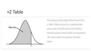
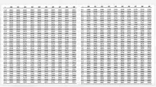
The Standardized NormalTable
• The Cumulative Standardized Normal table in the textbook gives the
probability less than a desired value of Z (i.e., from negative infinity
to Z)
Z
0 2.00
0.9772
Example:
P(Z < 2.00) = 0.9772
24.
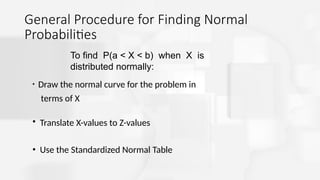
General Procedure forFinding Normal
Probabilities
• Draw the normal curve for the problem in
terms of X
• Translate X-values to Z-values
• Use the Standardized Normal Table
To find P(a < X < b) when X is
distributed normally:
25.
Finding Normal Probabilities
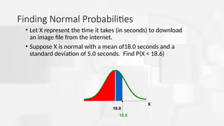
•Let X represent the time it takes (in seconds) to download
an image file from the internet.
• Suppose X is normal with a mean of18.0 seconds and a
standard deviation of 5.0 seconds. Find P(X < 18.6)
18.6
X
18.0
26.
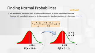
Finding Normal Probabilities
•Let X represent the time it takes, in seconds to download an image file from the internet.
• Suppose X is normal with a mean of 18.0 seconds and a standard deviation of 5.0 seconds. Find P(X
< 18.6)
Z
0.12
0
X
18.6
18
μ = 18
σ = 5
μ = 0
σ = 1
(continued)
0.12
5.0
8.0
1
18.6
σ
μ
X
Z
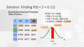
P(X < 18.6) P(Z < 0.12)
27.
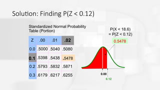
Z
0.12
0.5478
Standardized Normal Probability
Table(Portion)
0.00
= P(Z < 0.12)
P(X < 18.6)
Z .00 .01
0.0 .5000 .5040 .5080
.5398 .5438
0.2 .5793 .5832 .5871
0.3 .6179 .6217 .6255
.02
0.1 .5478
Solution: Finding P(Z < 0.12)
28.
Finding Normal
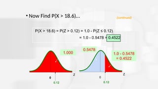
Upper TailProbabilities
• Suppose X is normal with mean 18.0 and standard deviation
5.0.
• Now Find P(X > 18.6)
X
18.6
18.0
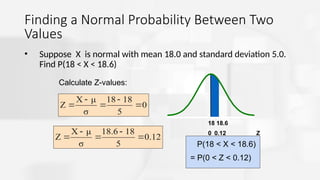
Finding a NormalProbability Between Two
Values
• Suppose X is normal with mean 18.0 and standard deviation 5.0.
Find P(18 < X < 18.6)
P(18 < X < 18.6)
= P(0 < Z < 0.12)
Z
0.12
0
X
18.6
18
0
5
8
1
18
σ
μ
X
Z
0.12
5
8
1
18.6
σ
μ
X
Z
Calculate Z-values:
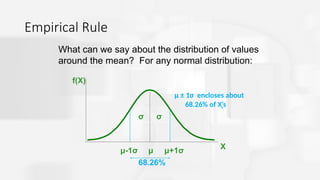
Empirical Rule
μ ±1σ encloses about
68.26% of X’s
f(X)
X
μ μ+1σ
μ-1σ
What can we say about the distribution of values
around the mean? For any normal distribution:
σ
σ
68.26%
33.
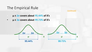
The Empirical Rule
•μ ± 2σ covers about 95.44% of X’s
• μ ± 3σ covers about 99.73% of X’s
x
μ
2σ 2σ
x
μ
3σ 3σ
95.44% 99.73%
(continued)
34.
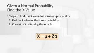
Given a NormalProbability
Find the X Value
• Steps to find the X value for a known probability:
1. Find the Z value for the known probability
2. Convert to X units using the formula:
Zσ
μ
X
35.
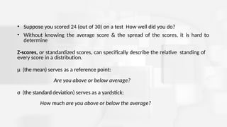
• Suppose youscored 24 (out of 30) on a test How well did you do?
• Without knowing the average score & the spread of the scores, it is hard to
determine
Z-scores, or standardized scores, can specifically describe the relative standing of
every score in a distribution.
μ (the mean) serves as a reference point:
Are you above or below average?
σ (the standard deviation) serves as a yardstick:
How much are you above or below the average?
36.
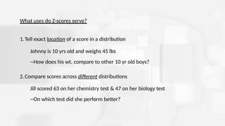
What uses doZ-scores serve?
1.Tell exact location of a score in a distribution
Johnny is 10 yrs old and weighs 45 lbs
--How does his wt. compare to other 10 yr old boys?
2.Compare scores across different distributions
Jill scored 63 on her chemistry test & 47 on her biology test
--On which test did she perform better?
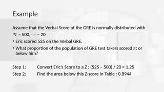
Example
Assume that theVerbal Score of the GRE is normally distributed with
= 500, = 20
• Eric scored 525 on the Verbal GRE.
• What proportion of the population of GRE test takers scored at or
below him?
Step 1: Convert Eric’s Score to a Z : (525 – 500) / 20 = 1.25
Step 2: Find the area below this Z-score in Table : 0.8944
43.
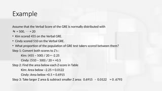
Example
Assume that theVerbal Score of the GRE is normally distributed with
= 500, = 20
• Kim scored 455 on the Verbal GRE.
• Cindy scored 510 on the Verbal GRE.
• What proportion of the population of GRE test takers scored between them?
Step 1: Convert both scores to Z’s :
Kim: (455 – 500) / 20 = -2.25
Cindy: (510 – 500) / 20 = +0.5
Step 2: Find the area below each Z-score in Table
Kim: Area below –2.25 = 0.0122
Cindy: Area below +0.5 = 0.6915
Step 3: Take larger Z area & subtract smaller Z area: 0.6915 - 0.0122 = 0 .6793
44.
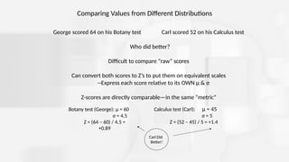
Comparing Values fromDifferent Distributions
George scored 64 on his Botany test Carl scored 52 on his Calculus test
Who did better?
Difficult to compare “raw” scores
Can convert both scores to Z’s to put them on equivalent scales
--Express each score relative to its OWN μ & σ
Z-scores are directly comparable—in the same “metric”
Botany test (George): μ = 60
σ = 4.5
Z = (64 – 60) / 4.5 =
+0.89
Calculus test (Carl): μ = 45
σ = 5
Z = (52 – 45) / 5 = +1.4
Carl Did
Better!
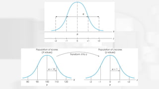
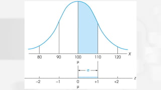
#37 Figure 5.3
The relationship between z-score values and locations in a population distribution.
Figure 5.5
An entire population of scores is transformed into z-scores. The transformation does not change the shape of the population, but the mean is transformed into a value of 0 and the standard deviation is transformed to a value of 1.
#38 Figure 5.6
Following a z-score transformation, the X-axis is relabeled in z-score units. The distance that is equivalent to 1 standard deviation on the X-axis (σ = 10 points in this example) corresponds to 1 point on the z-score scale.


![CTEV [ clubfoot] DR ARUN LAL ,DR MOHAMED ASHRAF travancore medical college k...](https://cdn.slidesharecdn.com/ss_thumbnails/ctevclubfootdrarunlaldrmohamedashraftravancoremedicalcollegekollamkeralaindia-260208063247-18fc466c-thumbnail.jpg?width=640&height=640&fit=bounds)

![ONFH[AVN HIP] -TRIPLE REGIME -A NOVAL SURGICAL CONCEPT .pptx](https://cdn.slidesharecdn.com/ss_thumbnails/onfhavnhip2026koaconcalicutdrgokuldevdrmashraf-260210064517-213ec005-thumbnail.jpg?width=640&height=640&fit=bounds)


