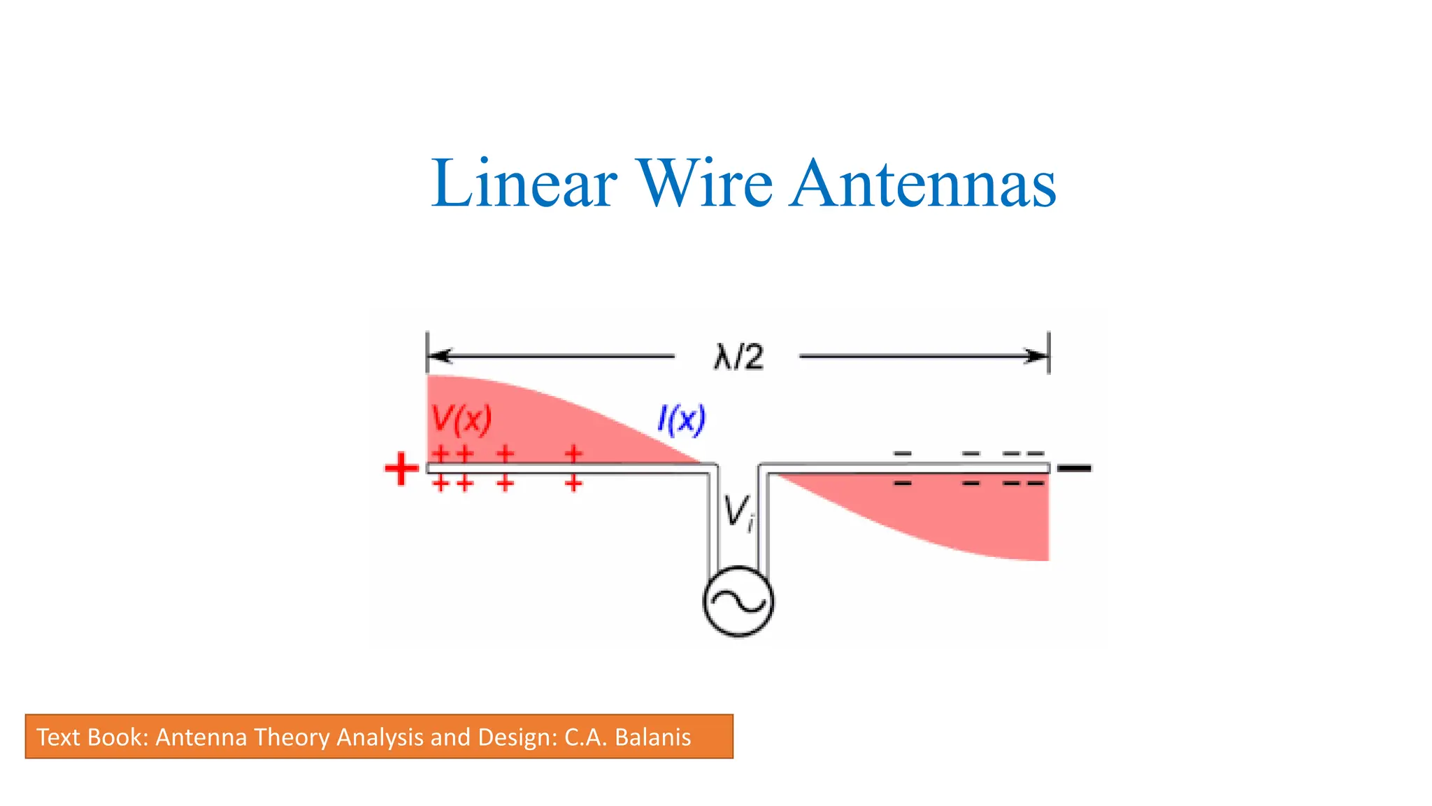
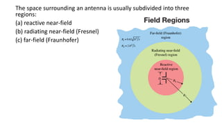
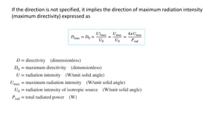
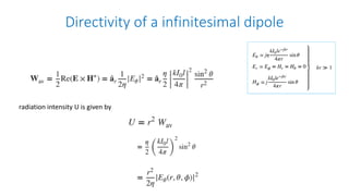
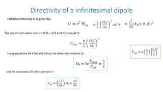
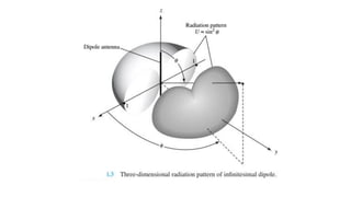
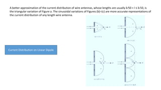
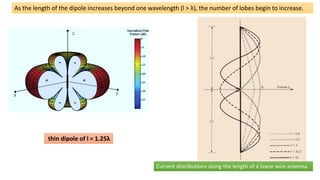
The document discusses antenna theory, focusing on the analysis and design of linear wire antennas, specifically detailing the characteristics and radiation patterns of Hertzian and finite dipoles. It covers topics such as the radiation resistance, directivity, current distribution, and the distinction between various field regions around antennas. Additionally, it explains the importance of the radiation pattern and introduces concepts like isotropic and directional patterns, contributing to a comprehensive understanding of antenna function and design.

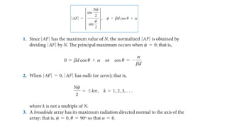


![3_Antenna Array [Modlue 4] (1).pdf](https://cdn.slidesharecdn.com/ss_thumbnails/3antennaarraymodlue41-220419112111-thumbnail.jpg?width=640&height=640&fit=bounds)


![Antenna lecture course CHapter 2_(2)[1].pdf](https://cdn.slidesharecdn.com/ss_thumbnails/antennach221-240525095938-532f47be-thumbnail.jpg?width=640&height=640&fit=bounds)


