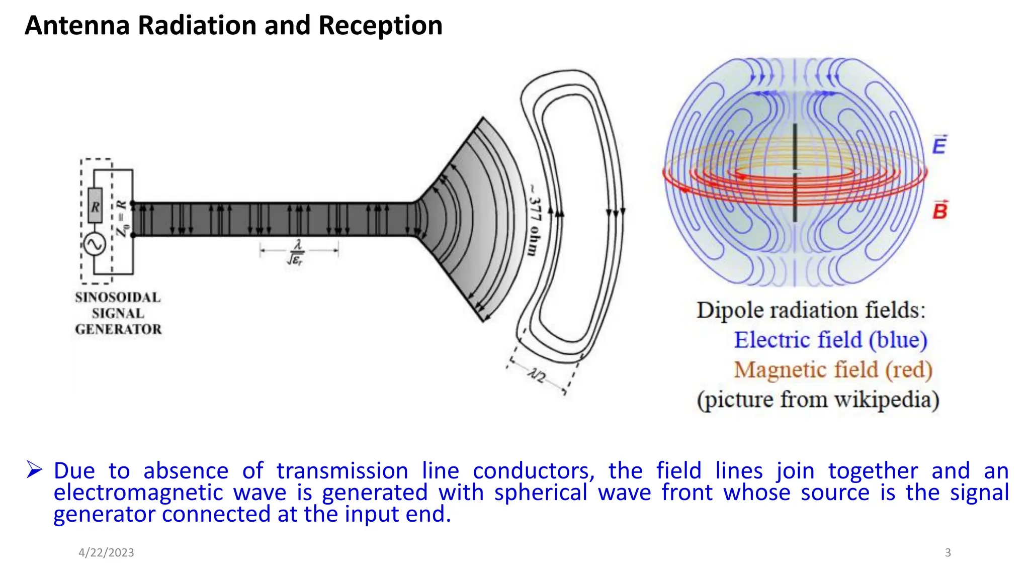
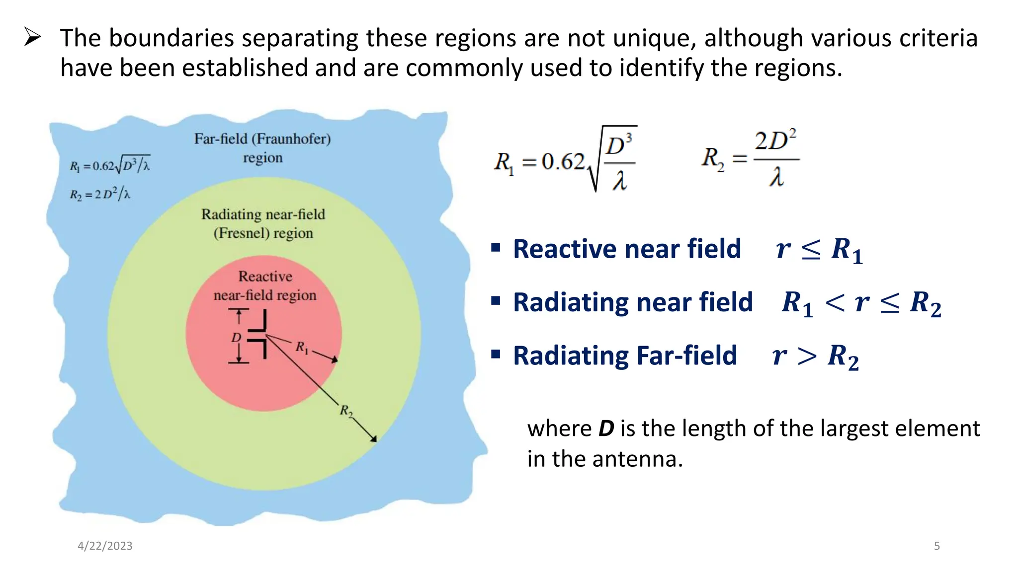
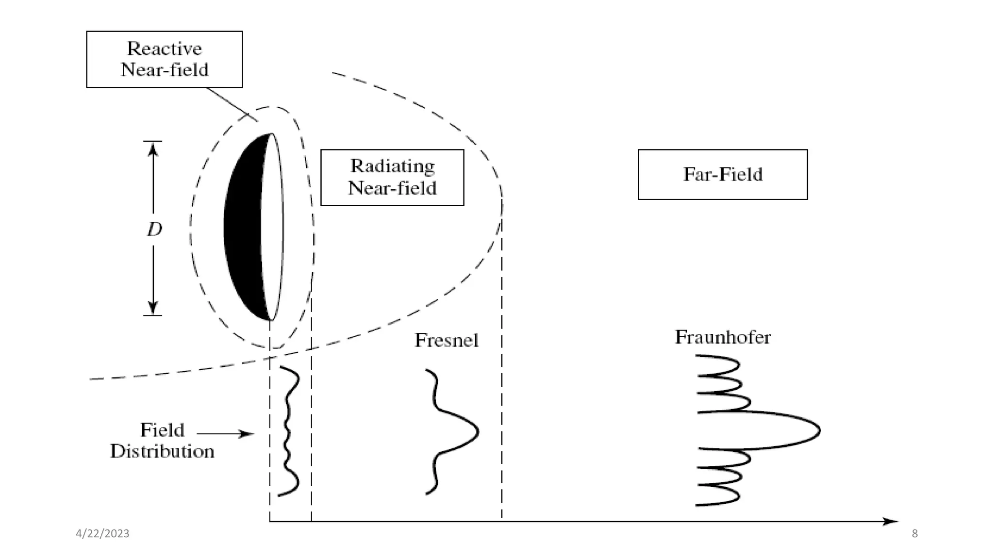
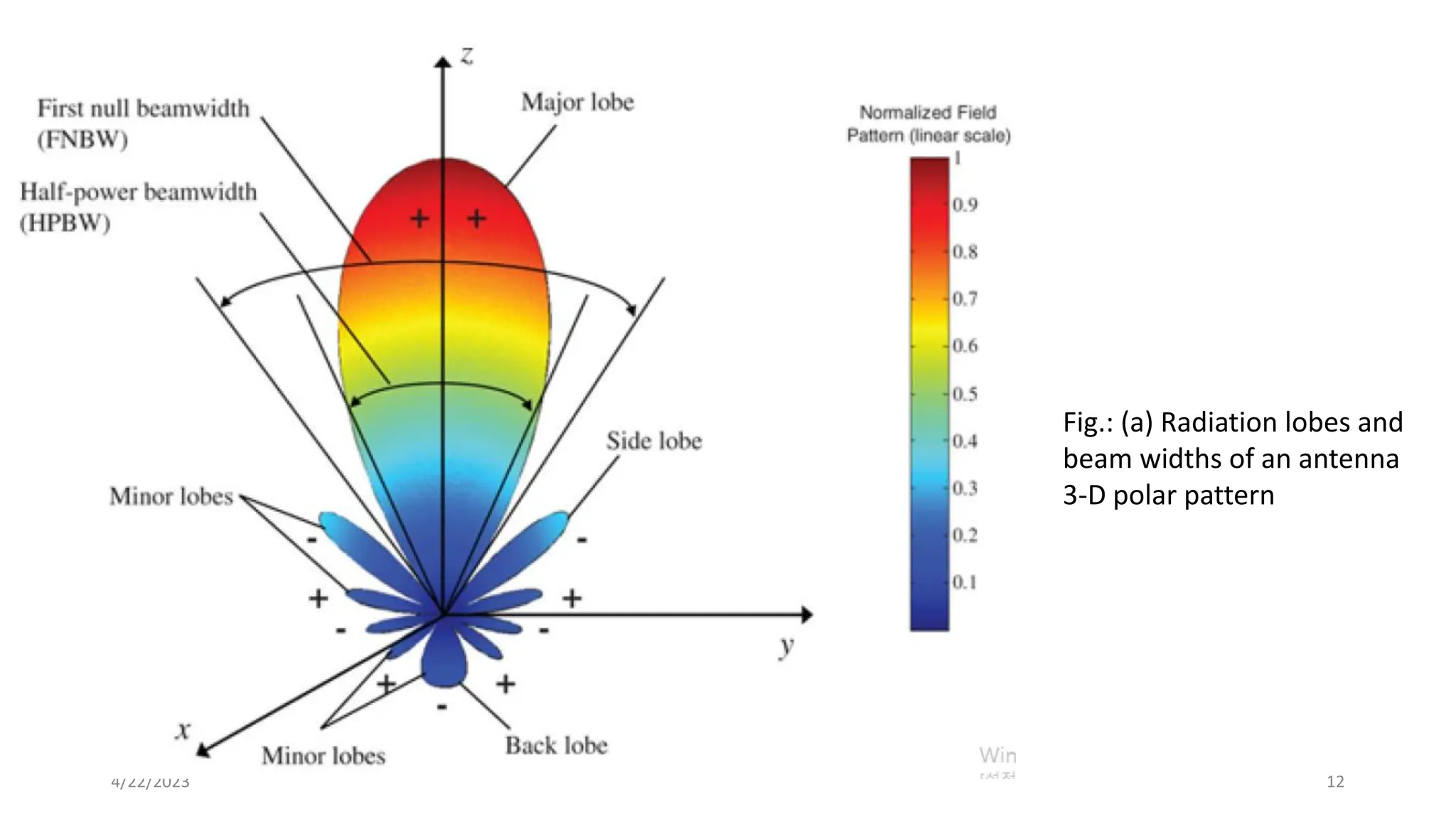
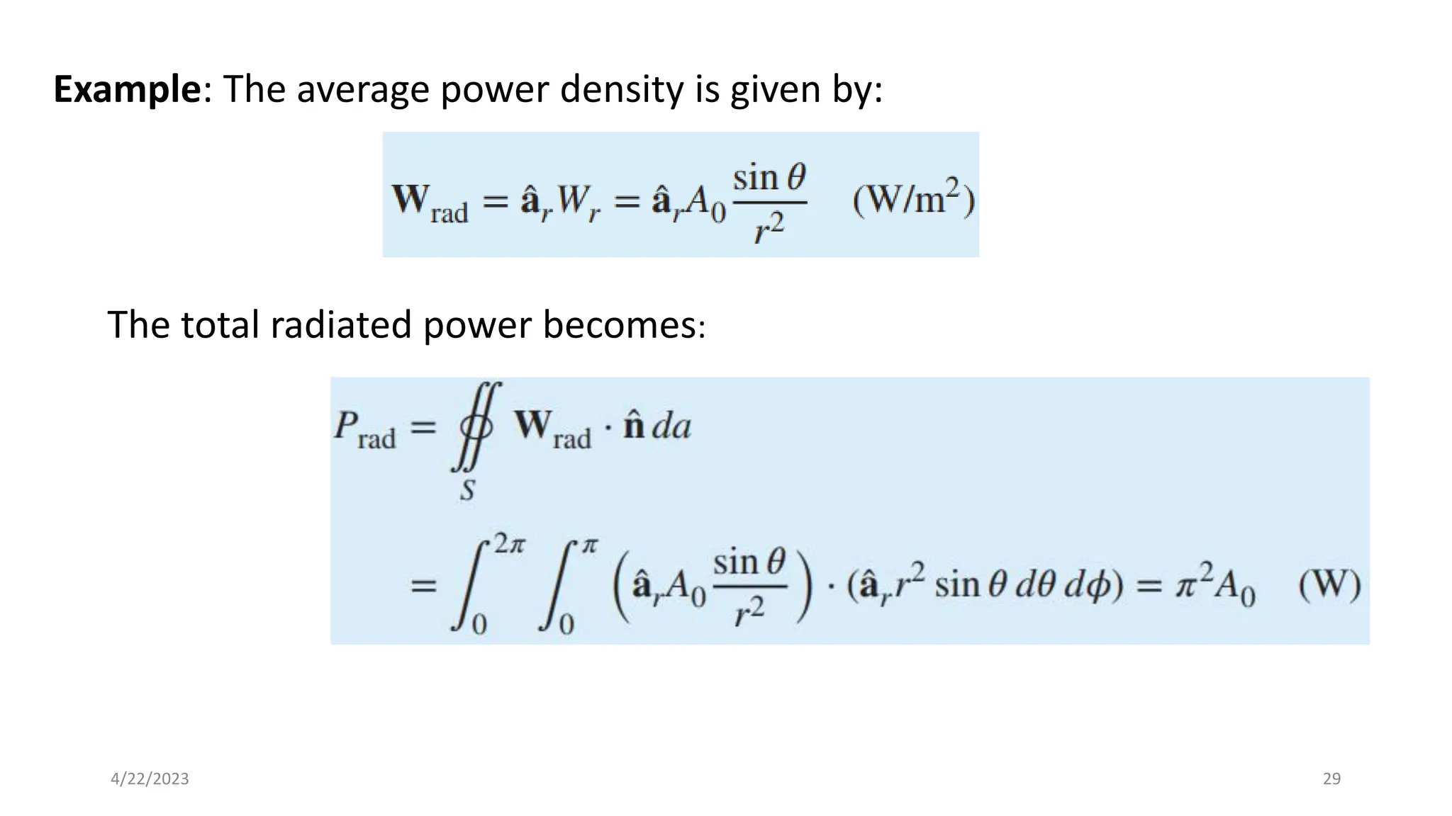
Antenna lecture course CHapter 2_(2)[1].pdf

Asossa University
Electrical and Computer Engineering Department
Post-Graduate Program
Advanced Antenna Systems
By: H/Maryam G.
Jan 18, 2023
1
4/22/2023

CHAPTER II
Antenna Parameters and Design Considerations
➢ Radiation Pattern
➢ Radiation Power Density and Radiation Intensity
➢ Beam width, Directivity and Gain
➢ Antenna Efficiency
➢ FRIIS Transmission Equation
➢ RF Radiation Hazards and Solutions
2
4/22/2023

Antenna Radiation and Reception
➢ Due to absence of transmission line conductors, the field lines join together and an
electromagnetic wave is generated with spherical wave front whose source is the signal
generator connected at the input end.
3
4/22/2023

Field Regions
➢ The field patterns generated by a radiating antenna vary with distance and
are associated with (i) radiating energy and (ii) reactive energy.
➢ The space surrounding an antenna is subdivided into three regions:
1. Reactive near-field
2. Radiating near-field (Fresnel) and
3. Radiating Far-field (Fraunhofer).
➢ The boundaries of these regions are not defined precisely but are only
approximations.
➢ Although no abrupt changes in the field configurations are noted as the
boundaries are crossed, there are distinct differences among them.
4
4/22/2023

➢ The boundaries separating these regions are not unique, although various criteria
have been established and are commonly used to identify the regions.
5
4/22/2023
▪ Reactive near field 𝒓 ≤ 𝑹𝟏
▪ Radiating near field 𝑹𝟏 < 𝒓 ≤ 𝑹𝟐
▪ Radiating Far-field 𝒓 > 𝑹𝟐
where D is the length of the largest element
in the antenna.

Reactive near-field region
➢ Is portion of the near-field region immediately surrounding the antenna where in
the reactive field predominates.
➢ For most antennas, the outer boundary of this region is commonly taken to exist
at a distance:
where λ is the wavelength (meter) and D is the largest dimension of the antenna (meter).
Radiating near-field (Fresnel) region
➢ Is region of the field of an antenna between the reactive near-field region and the
far-field region wherein radiation fields predominate and wherein the angular
field distribution is dependent upon the distance from the antenna.
➢ If the antenna has a maximum dimension that is not large compared to the
wavelength, this region may not exist.
6
4/22/2023

➢ For an antenna focused at infinity, the radiating near-field region is sometimes
referred to as the Fresnel region. The boundary for this region:
➢ In this region the field pattern is, in general, a function of the radial distance and
the radial field component may be substantial.
Far-field (Fraunhofer) region
➢ Is the region of the field of an antenna where the angular field distribution
is essentially independent of the distance from the antenna. It is commonly
taken to exist at distances.
➢ In this region, the field components are essentially transverse and the angular
distribution is independent of the radial distance where the measurements are made.
➢ Typical changes of antenna amplitude pattern shape from reactive near field toward
the far field. 7
4/22/2023

➢ The amplitude pattern of an antenna, as the observation distance is
varied from the reactive near field to the far field, changes in shape
because of variations of the fields, both magnitude and phase.
➢ A typical progression of the shape of an antenna, with the largest
dimension D, is shown in fig, It is apparent that in the reactive near field
region the pattern is more spread out and nearly uniform, with slight
variations.
➢ As the observation is moved to the radiating near-field region (Fresnel),
the pattern begins to smooth and form lobes.
➢ In the far-field region (Fraunhofer), the pattern is well formed, usually
consisting of few minor lobes and one, or more, major lobes.
9
4/22/2023

Radiation Pattern Lobes
➢ Once the electromagnetic (EM) energy leaves the antenna, the radiation
pattern tells us how the energy propagates away from the antenna.
➢ Radiation pattern is defined as a mathematical function or a graphical
representation of the radiation properties of the antenna as a function of space
coordinates.
➢ Various parts of a radiation pattern are referred to as lobes.
➢ A radiation lobe is a portion of the radiation pattern bounded by regions of
relatively weak radiation intensity.
➢ It is may be classified into major (main) and minor lobes. The minor lobe further
classified as side and back lobes.
➢ A major lobe also called main beam is defined as the radiation lobe containing
the direction of maximum radiation. In fig. below the major lobe is pointing in the
(𝜽 = 𝟎) direction.
➢ In some antennas, such as split-beam antennas, there may exist more than one
major lobe.
10
4/22/2023

➢ A minor lobe is any lobe except a major lobe. In figures (a) and (b) all the lobes
with the exception of the major can be classified as minor lobes.
➢ A side lobe is a radiation lobe in any direction other than the intended lobe.
Usually a side lobe is adjacent to the main lobe and occupies the hemisphere in
the direction of the main beam.
➢ A back lobe is a radiation lobe whose axis makes an angle of approximately
𝟏𝟖𝟎𝒐
with respect to the beam of an antenna. Usually it refers to a minor lobe
that occupies the hemisphere in a direction opposite to that of the major lobe.
▪ Fig: (a) demonstrates a symmetrical three dimensional polar pattern
with a number of radiation lobes. Some are of greater radiation
intensity than others, but all are classified as lobes.
▪ Fig: (b) illustrates a linear two-dimensional pattern where the same
pattern characteristics are indicated.
11
4/22/2023

12
4/22/2023
Fig.: (a) Radiation lobes and
beam widths of an antenna
3-D polar pattern

Fig: (b) Linear 2-D plot of power pattern and its associated lobes and beam widths.
13
4/22/2023

14
4/22/2023
Figure: Normalized three-dimensional
amplitude field pattern( in linear scale)

Radiation Pattern:
➢ In most cases, the radiation pattern is determined in the far-field
(Fraunhofer) region and is represented as a function of the directional
coordinates.
➢ Radiation properties include power density, radiation intensity, field
strength, directivity, phase or polarization.
➢ A convenient set of coordinates is shown in fig. below. A trace of the
received electric (magnetic) field at a constant radius is called the
amplitude field pattern.
➢ The radiation property of most concern is the two- or three dimensional
spatial distribution of radiated energy as a function of the observer’s
position along a path or surface of constant radius.
➢ On the other hand, a graph of the spatial variation of the power density
along a constant radius is called an amplitude power pattern.
15
4/22/2023

16
4/22/2023
Fig: Coordinate system for antenna analysis:

Radiation Pattern:
➢ Any field pattern can be represented in three dimensional spherical coordinates as
in fig. above or by plane cuts through the main lobe axis.
➢ Often the field and power patterns are normalized with respect to their maximum
value, resulting in normalized field and power patterns.
➢ Also, the power pattern is usually plotted on a logarithmic scale or more commonly
in decibels (dB).
➢ The normalized or relative patterns which are dimensionless quantities with
maximum value of unity are obtained by dividing the pattern component by its
maximum value.
➢ At distances that are large compared to the size of the antenna and the
wavelength, the shape of the field pattern is independent of distance.
➢ The patterns of interest are of this far-field condition, since in practice reception of
radiate antenna is in the far-field region.
➢ The normalized power pattern can be obtained by dividing the component of
power per unit area called Poynting vector to its maximum value.
17
4/22/2023

18
4/22/2023
➢We place an antenna at the center. The
electric field components are and
.
➢The radiated power will be in the
direction of the Poynting vector P = E X H.
Power pattern is . The normalized
power pattern is .
Normalized field
pattern
Normalized power
pattern

Figure: Two-dimensional normalized (a) field pattern (in linear scale) (b) power pattern
(in linear scale), and (c) power pattern (in dB)
19
4/22/2023

Radiation Pattern:
➢ Amplitude field pattern : A trace of the received electric/magnetic field at
a constant radius.
➢ Amplitude power pattern : A graph of the spatial variation of the power
density along a constant radius.
A. Field pattern (in linear scale): typically represents a plot of the
magnitude of the electric or magnetic field as a function of the angular
space.
B. Power pattern ( in linear scale): typically represents a plot of the square
of the magnitude of the electric or magnetic field as a function of the
angular space.
C. Power pattern (in dB): represents the magnitude of the electric or
magnetic field, in decibels, as a function of the angular space.
20
4/22/2023

21
4/22/2023
2
| E| -pattern
2
| E| -pattern in dB scale
|E|-pattern

Isotropic, Directional, and Omni-directional Patterns
22
4/22/2023
➢ Isotropic Antenna: A hypothetical lossless antenna pattern having equal
radiation in all directions.
▪ Ideal, not physically realizable.
▪ Often taken as a reference for expressing the directive properties of actual antennas.
➢ Directional Antenna: is one having the property of radiating or receiving
electromagnetic waves more effectively in some directions than in others.
▪ Examples of antennas with directional radiation patterns are horn antenna, dipole
antenna, etc.
➢ It is seen that the pattern in fig. below is non-directional in the azimuth plane
and directional in the elevation plane.
➢ This type of a pattern is designated as Omni-directional Antenna, and it is
defined as one having an essentially non-directional pattern in a given plane and
a directional pattern in any orthogonal plane.
▪ An Omni-directional pattern is special type of a directional pattern.

23
4/22/2023
Nondirectional Pattern
Directional Pattern
Orthogonal
Plane

24
4/22/2023
Fig: Sample of 2-D polar pattern.

Radian and Steradian
25
4/22/2023
➢ The measure of a plane angle is a radian.
One radian is defined as the plane angle
with its vertex at the center of a circle of
radius r that is subtended by an arc whose
length is r.
➢ The measure of a solid angle is a steradian.
One steradian is defined as the solid angle
with its vertex at the center of a sphere of
radius r that is subtended by a spherical
surface area equal to that of a square with
each side of length r.
➢ A graphical illustration is shown in fig
below.

Radian and Steradian
➢ Since the circumference of a circle of radius 𝑟 is 𝐶 = 2𝜋𝑟, there are
2𝜋 rad (2𝜋𝑟/𝑟) in a full circle. And since the area of a sphere of radius 𝑟
is 𝐴 = 4𝜋𝑟2, there are 4𝜋 sr (4𝜋𝑟2/𝑟2) in a closed sphere.
➢ The infinitesimal area 𝑑𝐴 on the surface of a sphere of radius r, shown in
fig above, is given by:
➢ Therefore, the element of solid angle 𝑑𝛺 of a sphere can be written as:
26
4/22/2023

Radiation Power density
➢ Electromagnetic waves are used to transport information through a wireless
medium or a guiding structure, from one point to the other.
➢ It is then natural to assume that power and energy are associated with
electromagnetic fields.
➢ The quantity used to describe the power associated with an electromagnetic
wave is the instantaneous Poynting vector defined as:
S = E X H*
where: S = Instantaneous power vector (W/m2)
E = instantaneous electric-field intensity (V/m)
H = instantaneous magnetic-field intensity (A/m)
➢ Since the Poynting vector is a power density, the total power crossing a closed
surface can be obtained by integrating the normal component of the Poynting
vector over the entire surface.
27
4/22/2023

➢ For time-harmonic EM fields:
➢ Poynting vector:
➢ Time average Poynting vector (average power density or radiation density):
▪ The Τ
1
2 factor appears because the E and H fields represent peak values, and it
should be omitted for RMS values:
➢ So that an Average power radiated power becomes:
28
4/22/2023

Example: The average power density is given by:
The total radiated power becomes:
29
4/22/2023

Radiation Intensity
➢ Radiation intensity in a given direction is defined as “the power radiated
from an antenna per unit solid angle.”
➢ The radiation intensity is a far-field parameter, and it can be obtained by
simply multiplying the radiation density by the square of the distance.
➢ In mathematical form it is expressed as:
where: U = radiation intensity (W/unit solid angle)
Wrad = radiation density (W/m2)
30
4/22/2023

Beamwidth
➢ It is defined as the angular separation between two identical points on
opposite side of the pattern maximum. In an antenna pattern, there are a
number of beamwidths.
➢ One of the most widely used beamwidths is the Half-Power Beamwidth
(HPBW), which is defined by IEEE as: “In a plane containing the direction of
the maximum of a beam, the angle between the two directions in which the
radiation intensity is one-half value of the beam.”
➢ Another important beamwidth is the angular separation between the first
nulls of the pattern, and it is referred to as the First-Null Beamwidth
(FNBW).
➢ Both the HPBW and FNBW are demonstrated for the pattern in Figure
However, in practice, the term beamwidth, with no other identification,
usually refers to HPBW.
31
4/22/2023

➢ The beamwidth of an antenna is a very important figure of merit and often
is used as a trade-off between it and the side lobe level; As the beamwidth
decreases, the side lobe increases and vice versa.
➢ The most common resolution criterion states that the resolution capability
of an antenna to distinguish between two sources is equal to half the first-
null beamwidth (FNBW/2), which is usually used to approximate the half
power beamwidth (HPBW).
➢ That is, two sources separated by angular distances equal or greater than
FNBW/2 ≈ HPBW of an antenna with a uniform distribution.
➢ If the separation is smaller, then the antenna will tend to smooth the
angular separation distance.
➢ Example: Refer example 2.4 in your text book (ANTENNA THEORY, 4th edition by:
Constantine A. Balanis).
32
4/22/2023

Directivity
➢ Directivity is a measure of the antenna‘s ability to focus the energy in one or
more specific directions.
➢ Directivity of an antenna defined as the ratio of the radiation intensity in a
given direction from the antenna to the radiation intensity averaged over
all directions.
➢ The average radiation intensity is equal to the total power radiated by the
antenna divided by 4π.
➢ If the direction is not specified, the direction of maximum radiation intensity
is implied.
➢ Stated more simply, the directivity of a non isotropic source is equal to the
ratio of its radiation intensity in a given direction over that of an isotropic
source.
33
4/22/2023

➢ In mathematical form, it can be written as:
➢ If direction is not mentioned, it implies the direction of maximum
radiation intensity, maximum directivity is expressed as:
where:
34
4/22/2023

Gain
➢ Defined as the ratio of the intensity, in a given direction, to the radiation
intensity that would be obtained if the power accepted by the antenna were
radiated isotopically.
➢ The gain of the antenna is closely related to the directivity, it is a measure
that takes into account the efficiency of the antenna as well as its directional
capabilities.
➢ The radiation intensity corresponding to the isotopically radiated power is
equal to the power accepted (input) by the antenna divided by 4π. In
equation form this can be expressed as:
35
4/22/2023

Bandwidth
➢ The bandwidth of an antenna is defined as the range of frequencies within which
the performance of the antenna, with respect to some characteristic, conforms to
a specified standard.
➢ The bandwidth can be considered to be the range of frequencies, on either side of
a centre frequency (usually the resonance frequency for a dipole), where the
antenna characteristics are within an acceptable value of those at the centre
frequency.
▪ For broadband antennas, the bandwidth is usually expressed as the ratio of the
upper-to-lower frequencies of acceptable operation.
▪ Example: a 10:1 bandwidth indicates: upper frequency is 10 times greater than the lower.
➢ For narrowband antennas, the bandwidth is expressed as a percentage of the
frequency difference (upper minus lower) over the centre frequency of the
bandwidth.
▪ Example: a 5% bandwidth indicates that the frequency difference of acceptable operation is
5% of the centre frequency of the bandwidth.
36
4/22/2023

Polarization
➢ Polarization is defined as the
property of an EM wave describing
the time-varying direction and
relative magnitude of the E-field
vector.
➢ In other words, Polarization of
radiated wave describes the
oscillation direction and relative
magnitude of the electric field.
➢ Specifically, the figure traced as a
function of time by the extremity
of the vector at a fixed location in
space, and the sense in which it is
traced, as observed along given
direction.
37
4/22/2023
Fig: Polarization of EM waves

38
4/22/2023
(a) Linear polarization (b) Circular polarization and (c) Elliptical polarization
• Blue line : Electric field of a radiated/received wave
• Red and green line : Consisting of (one) two orthogonal, in-phase components
• Purple line : Polarized along a plane
(a) (b) (c)

➢ Polarization may be classified as linear, circular, or elliptical.
➢ If the vector that describes the electric field at a point in space as a function
of time is always directed along a line, the field is said to be linearly
polarized.
➢ In general, however, the figure that the electric field traces is an ellipse, and
the field is said to be elliptically polarized.
➢ Linear and circular polarizations are special cases of elliptical, and they can
be obtained when the ellipse becomes a straight line or a circle, respectively.
➢ The figure of the electric field is traced in a clockwise (CW) or
counterclockwise (CCW) sense. Clockwise rotation of the electric-field vector
is also designated as right-hand polarization and counterclockwise as left-
hand polarization.
39
4/22/2023

Input Impedance
➢ Input impedance is defined as the impedance presented by an antenna at
its input terminals or the ratio of the voltage to current at a pair of input
terminals or the ratio of the appropriate components of the electric to
magnetic fields at a point.
Fig: Transmitting antenna and its equivalent circuits.
40
4/22/2023
Loss
resistance
Radiation
resistance
g g g
Z R jX
= +
= Generator impedance (ohms)
= Resistance of generator impedance (ohms)
= Reactance of generator impedance (ohms)
g
Z
g
R
g
X

➢ The ratio of the voltage to current at these terminals (designated as a-b),
with no load attached, defines the impedance of the antenna as:
𝒁𝑨 = 𝑹𝑨 + 𝒋𝑿𝑨
Where: 𝑍𝐴 = antenna impedance at terminals a–b, (Ω)
𝑅𝐴 = antenna resistance at terminals a–b , (Ω)
𝑋𝐴 = antenna reactance at terminals a–b, (Ω)
➢ Input impedance at a pair of terminals which are the input terminals of
the antenna. In Fig. above these terminals are designated as a − b.
41
4/22/2023

➢ To find the amount of power delivered to 𝑹𝒓 for radiation and the amount
dissipated in 𝑹𝑳 as heat.
42
4/22/2023
( ) ( )
g g
g
t r L g A g
V V
I
Z R R R j X X
= =
+ + + +
1
2 2 2
( ) ( )
g
g
r L g A g
V
I
R R R j X X
==
 
+ + + +
 
2
2
2 2
1
2 2 ( ) ( )
g r
r g r
r L g A g
V R
P I R
R R R j X X
 
 
= =
 
+ + + +
 
 
 
2
2
2 2
1
2 2 ( ) ( )
g L
L g L
r L g A g
V R
P I R
R R R j X X
 
 
= =
 
+ + + +
 
 
 
➢ Power delivered to the antenna for radiation.
➢ Power that dissipated as heat.
➢ Maximum power delivered to the
antenna when conjugate matching.
➢ Conjugate matching;
r L g
R R R
+ =
A g
X X
= −

43
4/22/2023
2 2
2 2
2 4( ) 8 ( )
g g
r r
r
r L r L
V V
R R
P
R R R R
   
= =
   
+ +
   
2
2
8 ( )
g L
L
r L
V R
P
R R
 
=  
+
 
2 2 2
2
1
8 ( ) 8 8
g g g
g
g
r L r L g
V V V
R
P
R R R R R
   
= = =
   
+ +
   
2 2
2 2
8 ( ) 8 ( )
g g
g r L
g r L
r L r L
V V
R R R
P P P
R R R R
   
+
= + = =
   
+ +
   
➢ Power that dissipated as heat in the internal resistance of the generator = power for
radiation + power that dissipated as heat in the antenna.
➢ If the antenna is lossless and matched to the transmission line half of the total power supplied by the
generator is radiated by the antenna during conjugate matching, and the other half is dissipated as heat in
the generator.
1 ( 0)
r
cd L
r L
R
e R
R R
 
= = =
 
+
 

44
4/22/2023
➢ Conjugate matching ( to remove imaginary components)
r L T A T
R R R X X
+ = = −
▪ Power delivered to the load 𝑹𝑻 :
▪ Power that scattered of (re-radiated):
▪ Power that dissipated as heat through 𝑹𝑳 :
2 2 2
2
1
8 ( ) 8 8
T T T
T
T
r L r L T
V V V
R
P
R R R R R
   
= = =
   
+ +
   
2 2
2 2
2 4( ) 8 ( )
T T
r r
r
r L r L
V V
R R
P
R R R R
   
= =
   
+ +
   
2
2
8 ( )
T L
L
r L
V R
P
R R
 
=  
+
 
Which is collected or captured Power

Antenna Radiation Efficiency
➢ The antenna efficiency that takes into account the reflection, conduction,
and dielectric losses.
➢ The conduction and dielectric losses of an antenna are very difficult to
compute and in most cases they are measured.
➢ Even with measurements, they are difficult to separate and they are usually
lumped together to form the ecd efficiency.
➢ The resistance 𝑅𝐿 is used to represent the conduction-dielectric losses.
➢ The conduction-dielectric efficiency ecd is defined as the ratio of the power
delivered to the radiation resistance 𝑅𝑟 to the power delivered to 𝑅𝑟and
𝑅𝐿. It is given by:
45
4/22/2023

Antenna Efficiency
➢ The power efficiency of an antenna or antenna efficiency is the ratio of power radiated to
total power input to the antenna. Thus, if the radiation resistance 𝑹𝒓 and the loss
resistance 𝑹𝑳 is known, the antenna efficiency can expressed as:
▪ Here, I is the current flowing through the antenna terminals. Multiplying 𝜼𝒂 by 100,
one may obtain the percentage antenna efficiency.
➢ The total antenna efficiency e0 is used to take into account losses at the input
terminals and within the structure of the antenna. Such losses may be due to:
➢ Reflections because of the mismatch between the transmission line and the antenna.
➢ I 2R losses (conduction and dielectric).
46
4/22/2023

Fig: Reference terminals and antenna losses.
47
4/22/2023
➢ In general, the overall
efficiency can be written
as:
e0 = ereced

FRIIS Transmission Equation
➢ The FRIIS Transmission Equation relates the power received to the power
transmitted between two antennas separated by a distance:
.…………… (far-field region)
where: D is the largest dimension of either antenna.
48
Prepared by: H/MARYAM G.
08/05/2013 E.C

➢ FRIIS Transmission Equation is expressed by:
where: , is the gain of antenna (dimensionless)
, is power density ( Τ
𝑊𝑎𝑡𝑡 𝑚2
)
, is total received power (Watt)
49
08/05/2013 E.C

Example
1. The normalized radiation intensity of an antenna is represented by:
𝑢 𝜃 = 𝑐𝑜𝑠2
𝜃 𝑐𝑜𝑠2
3𝜃 ; (0 ≤ 𝜃 ≤ 900
, 0 ≤ 𝜙 ≤ 3600
)
a. Find HPBW (in degrees and radians)
b. Find FNBW (in degrees and radians)
2. If the impedance of a horn antenna is (𝑍𝐴= 20 + 𝑗30) Ω and the characteristics
impedance of 50 Ω, then evaluate voltage reflection coefficient at the input
terminal of the antenna and calculate the overall voltage standing wave ratio?
3. A GSM1800 cell tower antenna is transmitting 20 W of power in the frequency
range of 1840 to 1845 MHz. The gain of the antenna is 17 dB. Find the power
density at a distance of (a) 50 m and (b) 300 m in the direction of maximum
radiation.
4. The transmitting and receiving antennas are separated by a distance of 200 𝜆 and
have directive gains of 25 and 18 dB, respectively. If 5 mW of power is to be
received, calculate the minimum transmitted power.
50
08/05/2013 E.C

Solution:
1. Ans: a) HPBW ≈ 0.5 rad; ≈ 28.650
b) FNBW ≈ 1.047 rad; ≈ 600
2. Ans: Γ = −0.206 + 𝑗 0.517 = 0.56∠1120; VSWR = 3.55
3. Power density:
4. Minimum transmitted power:
Given that 𝐺𝑡 𝑑𝐵 = 25𝑑𝐵 = 10𝑙𝑜𝑔10 𝐺𝑡 ; 𝐺𝑡 = 102.5 = 316.23
Similarly, 𝐺𝑟 𝑑𝐵 = 18𝑑𝐵 = 10𝑙𝑜𝑔10 𝐺𝑟 ; 𝐺𝑟 = 101.8
= 63.1
Using the FRIIS equation, we have: 𝑃𝑟 = 𝐺𝑡 𝐺𝑟
𝜆
4𝜋𝑟
2
𝑃𝑡 ; 𝑃𝑡 = 𝑃𝑟
4𝜋𝑟
𝜆
2 1
𝐺𝑡 𝐺𝑟
= 𝟏. 𝟓𝟖𝟑 𝑊
51
08/05/2013 E.C

Potential Solutions
63
4/22/2023

Any Questions?
END !
64
4/22/2023

Antenna lecture course CHapter 2_(2)[1].pdf

More Related Content

Similar to Antenna lecture course CHapter 2_(2)[1].pdf

More from AbrahamGadissa

Recently uploaded

Antenna lecture course CHapter 2_(2)[1].pdf