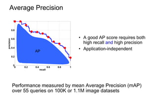
Download as PDF, PPTX


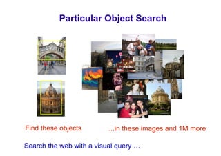
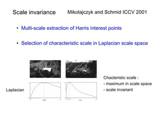
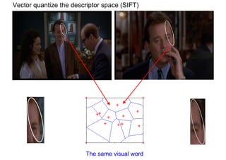
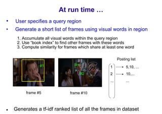
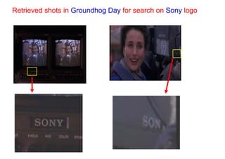
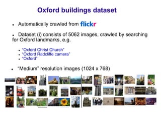
![Problem specification: particular object retrieval
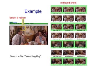
Example: visual search in feature films
Visually defined query “Groundhog Day” [Rammis, 1993]
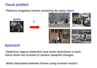
“Find this
clock”
“Find this
place”](https://image.slidesharecdn.com/azpart1a-110802082200-phpapp02/85/Andrew-Zisserman-Talk-Part-1a-4-320.jpg)
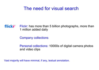
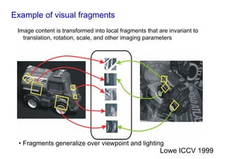
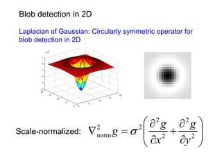
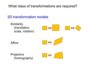
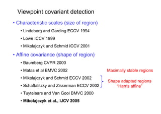
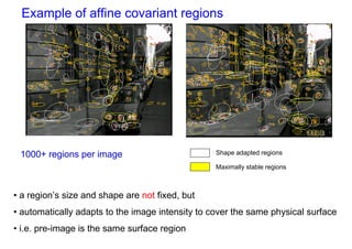
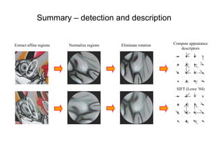
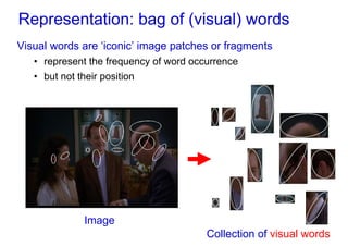
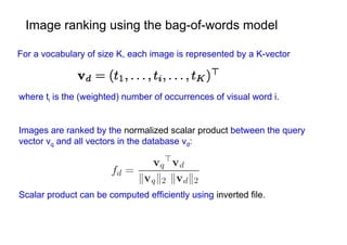
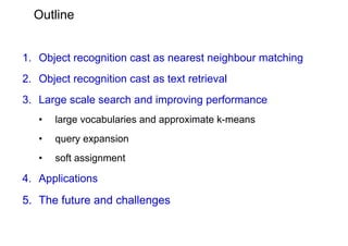
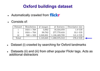
![Viewpoint invariant description
• Elliptical viewpoint covariant regions
• Shape Adapted regions
• Maximally Stable Regions
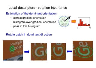
• Map ellipse to circle and orientate by dominant direction
• Represent each region by SIFT descriptor (128-vector) [Lowe 1999]
• see Mikolajczyk and Schmid CVPR 2003 for a comparison of descriptors](https://image.slidesharecdn.com/azpart1a-110802082200-phpapp02/85/Andrew-Zisserman-Talk-Part-1a-34-320.jpg)
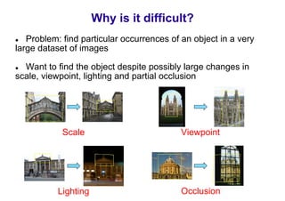
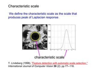
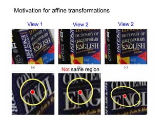
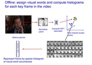
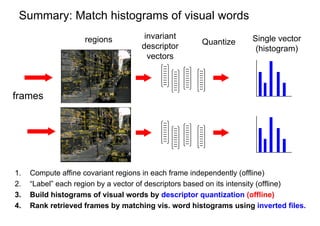
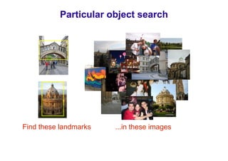
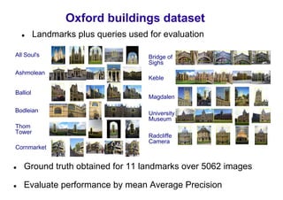
![Descriptors – SIFT [Lowe’99]
distribution of the gradient over an image patch
image patch gradient 3D histogram
x
→ →
y
4x4 location grid and 8 orientations (128 dimensions)
very good performance in image matching [Mikolaczyk and Schmid’03]](https://image.slidesharecdn.com/azpart1a-110802082200-phpapp02/85/Andrew-Zisserman-Talk-Part-1a-36-320.jpg)
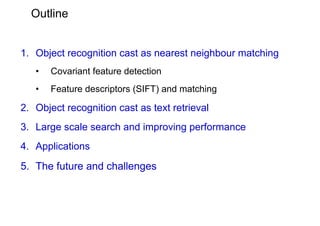
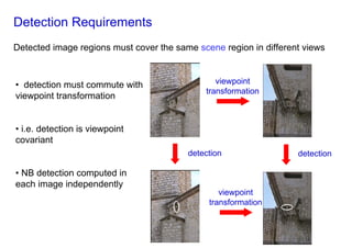
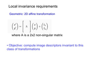
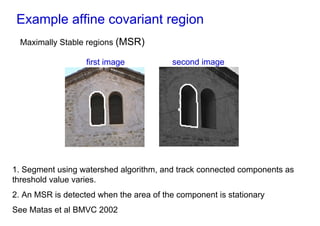
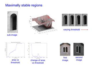
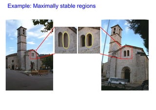
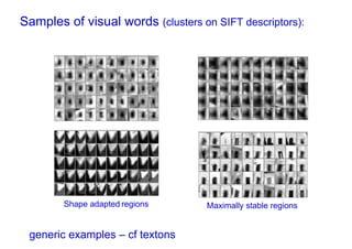
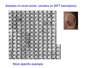
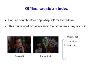
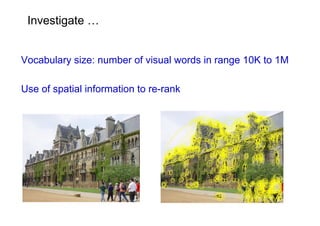
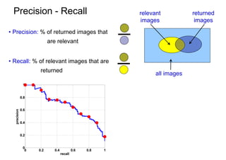
![Example
In each frame independently
determine elliptical regions (detection covariant with camera viewpoint)
compute SIFT descriptor for each region [Lowe ‘99]
1000+ descriptors per frame
Harris-affine
Maximally stable regions](https://image.slidesharecdn.com/azpart1a-110802082200-phpapp02/85/Andrew-Zisserman-Talk-Part-1a-40-320.jpg)

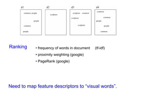
![Text retrieval lightning tour
Stemming Represent words by stems, e.g. “walking”, “walks” “walk”
Stop-list Reject the very common words, e.g. “the”, “a”, “of”
Inverted file
Ideal book index: Term List of hits (occurrences in documents)
People [d1:hit hit hit], [d4:hit hit] …
Common [d1:hit hit], [d3: hit], [d4: hit hit hit] …
Sculpture [d2:hit], [d3: hit hit hit] …
• word matches are pre-computed](https://image.slidesharecdn.com/azpart1a-110802082200-phpapp02/85/Andrew-Zisserman-Talk-Part-1a-45-320.jpg)
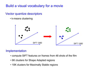
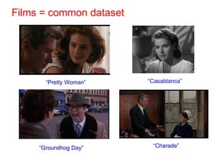
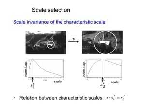
![Bag of visual words particular object retrieval
centroids
Set of SIFT (visual words)
query image descriptors
sparse frequency vector
Hessian-Affine visual words
regions + SIFT descriptors +tf-idf weighting
Inverted
file
querying
Geometric ranked image
verification short-list
[Chum & al 2007] [Lowe 04, Chum & al 2007]](https://image.slidesharecdn.com/azpart1a-110802082200-phpapp02/85/Andrew-Zisserman-Talk-Part-1a-93-320.jpg)

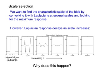
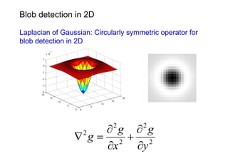
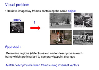
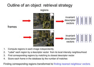
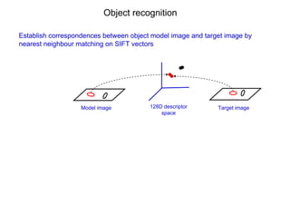
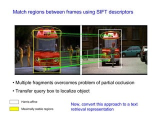
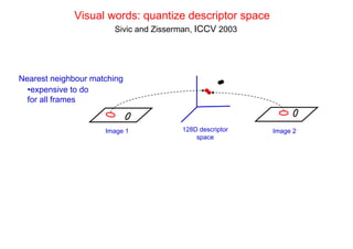
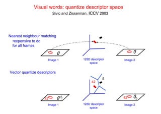
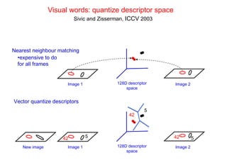
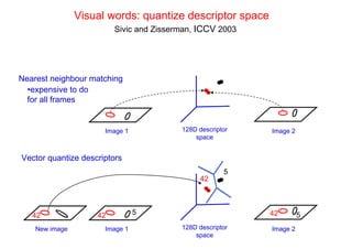
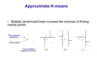
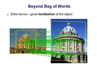
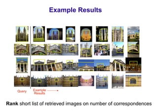
This document discusses visual search and recognition, specifically large scale instance search. It outlines detecting objects across different images despite changes in scale, viewpoint, lighting and occlusion. Key steps include covariant feature detection to find corresponding regions, and generating invariant descriptors like SIFT to match features between images. The goal is to cast object recognition as nearest neighbor matching or text retrieval to perform efficient search over very large datasets.