Download to read offline


![Consider the following example.
"
3 1
1 2
#
·
"
x1
x2
#
=
"
5
5
#
We can multiply the second row by -3 to obtain the following.
"
3 1
−3 −6
#
·
"
x1
x2
#
=
"
5
−15
#
The following is obtained when we add the first row to the second row.
"
3 1
0 −5
#
·
"
x1
x2
#
=
"
5
−10
#
The equation is now in upper triangular form, making it easy to solve the simulta-
neous equations and obtain the values of x1 and x2. More specifically, the second
row tells us that −5x2 = −10, giving x2 = 2. The first row reveals that 3x1 +x2 = 5.
Substituting for x2 and solving yields x1 = 1. Of course, more steps are required
when N is greater and that’s where your Matlab skills come in to play!
Draw a flow chart and write some Matlab code for a function that obtains the
upper triangular form by manipulating A and b into A′
and b′
, respectively. Your
function must also obtain the solution vector x for the simultaneous equations.
Therefore, the first line of your Matlab function is required to be as follows.
function [x, Aprime, bprime] = solve(A, b)
In cases where no errors occur, x and bprime are required to have the same di-
mensions as b, while Aprime is required to have the same dimensions as A.
Try your function with the following six tests (some of which have particular
features that will challenge your function’s error checking).
1. A =
1 1 0
2 1 1
1 2 3
, b =
3
7
14
.
2. A =
0 1 3 2
2 1 4 0
1 1 2 1
1 2 3 1
, b =
14
11
11
15
.
3. A =
1 1 3
1 1 1
2 1 1
, b =
4
2
3
.
4](https://image.slidesharecdn.com/assignmentonmatlab-230807142932-1c5cea51/75/Assignment-On-Matlab-4-2048.jpg)


![Exercise 2
The mathematical function y = f(x) has one dependent variable y, but N indepen-
dent variables, which are provided in the vector x = [x1, x2, x3, . . . , xN]. Suppose
that you want to find the particular values of the independent variables x that max-
imise the value of the dependent variable y. However, consider the case where the
function is like a ‘black box’; you can input some particular values of the indepen-
dent variables x and observe the resultant value of the dependent variable y, but
you can’t see how the function is defined. Since you don’t know how the value of
y depends on those of x, you are prevented from using differentiation techniques
to find the particular values of x that maximise the value of y. In this case, the
steepest ascent optimisation algorithm comes to the rescue!
The steepest ascent optimisation algorithm is an iterative algorithm for finding the
particular values of x that maximise the value of y = f(x). This algorithm starts
with a 1 by N vector of initial values for the independent variables x0. It then
assesses the gradient of the function f(x) in the vicinity of these values x0. Note
that this gradient g0 = ∇ f(x0) has direction has well as magnitude and so g0 is
also a 1 by N vector, just like x0. The direction of the gradient g0 points ‘uphill’,
towards better values of the independent variables x, which give higher values
for y = f(x). This allows us to easily replace our initial independent variable
values x0 with new better ones x1. More specifically, we can obtain x1 according
to xi = xi−1 + δ · gi−1, where δ is a small positive constant. Furthermore, we can
iteratively repeat this process to improve upon x1 and so on. This iterative process
can be terminated when f(xi) − f(xi−1) < t, where t is another small positive
threshold constant.
The steepest ascent optimisation algorithm is exemplified in Figure 2, in which
a surface plot is provided for a function y = f1(x) of two independent variables
x = [x1, x2]. In this example, the algorithm used initial independent variable
values of x0 = [0.5, −0.9] and it ran for 25 iterations. The evolution of these
iterations is indicated using a series of linked dots, which plots yi = f1(xi) against
xi for i = 0, 1, 2, . . . , 25. As shown in Figure 2 the algorithm always progresses
‘uphill’, in the direction of the gradient gi. Furthermore, the algorithm progresses
at a rate which is proportional to the magnitude of the gradient gi, by a coefficient
equal to δ = 0.25. As a result, big hops are used when the gradient is steep, but
small hops are used when approaching the highest point of the surface plot. In this
way, the steepest ascent optimisation algorithm is able to quickly and accurately
determine the values of x that maximises the function y = f1(x).
In this exercise, you need to use Matlab to perform steepest ascent optimisation
8](https://image.slidesharecdn.com/assignmentonmatlab-230807142932-1c5cea51/75/Assignment-On-Matlab-8-2048.jpg)
![−1
−0.5
0
0.5
1 −1
−0.5
0
0.5
1
0
0.5
1
1.5
finish
y
x1
x2
start
Figure 2: Example of using the steepest ascent optimisation algorithm to max-
imise y = f1(x). Here, x = [x1, x2], x0 = [0.5, −0.9] and δ = 0.25.
9](https://image.slidesharecdn.com/assignmentonmatlab-230807142932-1c5cea51/75/Assignment-On-Matlab-9-2048.jpg)
![and find the independent variable values that maximise the mathematical functions
that are listed below. You will need to write a Matlab function for each of these
mathematical functions. Each of these Matlab functions is required to have a
first line like the following example, which should be used for the first of the
mathematical functions listed below, y = f1(x).
function y = f_1(x)
Here, the argument x is required to be a 1 by N vector that provides the indepen-
dent variables x = [x1, x2, x3, . . . , xN]. Furthermore, y is required to be a scalar
that returns the corresponding value of y = f1(x).
You will also need to draw a flow chart and write a Matlab function for performing
the steepest ascent optimisation algorithm. Note that your single Matlab function
is required to work for all three of the mathematical functions listed below. The
first line of your Matlab function is required to be as follows.
function [X, y] = optimise(function_name, x_0, delta)
Here, the argument function name is a function handle that allows you to specify
which of the mathematical functions listed below to optimise. More specifically,
this argument provides a string containing the name your corresponding Matlab
function. For example, this string would have a value of ’f 1’, if the mathemat-
ical function y = f1(x) was to be optimised. The argument x 0 lets you specify
the vector of initial independent variable values x0, as described above. The third
argument delta is used to provide a value for the small positive scalar δ, which
controls how far the steepest ascent algorithm will hop in each iteration. Your
optimise function is required to have two return variables. The first X should be
an M by N matrix, where M is the number of iterations that the steepest ascent
algorithm runs for. Each row of the matrix X should provide the vector of inde-
pendent variable values xi that was used in a different iteration. More specifically,
x0 should provide the first row of X, x1 should provide the second row and so on.
The second return variable y should be an M by 1 vector that provides the cor-
responding dependent variable values yi, where the first element provides y0, the
second provides y1 and so on.
Write Matlab functions for each of the following three mathematical functions
and use them as inputs to your optimise function.
1. y = f1(x),
x = [x1, x2],
x0 = [0.5, −0.9],
f1(x1, x2) = 1 − x2
1/4 − x2
2/4 − sin(−2x1 − 3x2)/2,
δ = 0.25.
10](https://image.slidesharecdn.com/assignmentonmatlab-230807142932-1c5cea51/75/Assignment-On-Matlab-10-2048.jpg)
![2. y = f2(x),
x = [x1],
x0 = [220],
f2(x1) = 9.87 sin(2b(x1)) − 7.53 cos(b(x1)) − 1.5 sin(b(x1)),
b(x1) = 2π(x1 − 81)/365,
δ = 50.
3. y = f3(x),
x = [x1, x2, x3],
x0 = [0, 0, 0],
f3(x1, x2, x3) = 9x1 + 8x2 + 7x3 − 6x2
1 − 5x2
2 − 4x2
3 + 3x1x2 + 2x1x3 + x2x3,
δ = 0.1.
Include listings of your f 1, f 2 and f 3 Matlab functions in your write-up.
Also include your flow chart and a listing of your optimise function. Take
the results you obtained by passing your f 1 function to your optimise func-
tion and use Matlab to draw a 3D figure similar to Figure 2. Similarly, draw
an equivalent 2D plot for the results obtained using your f 2 function. In ad-
dition to these plots, your write-up should include the matrix X and the vector
y that you obtained by passing your f 3 function to your optimise function.
Here is some advice for completing this exercise:
• Begin by writing the Matlab functions f 1, f 2 and f 3.
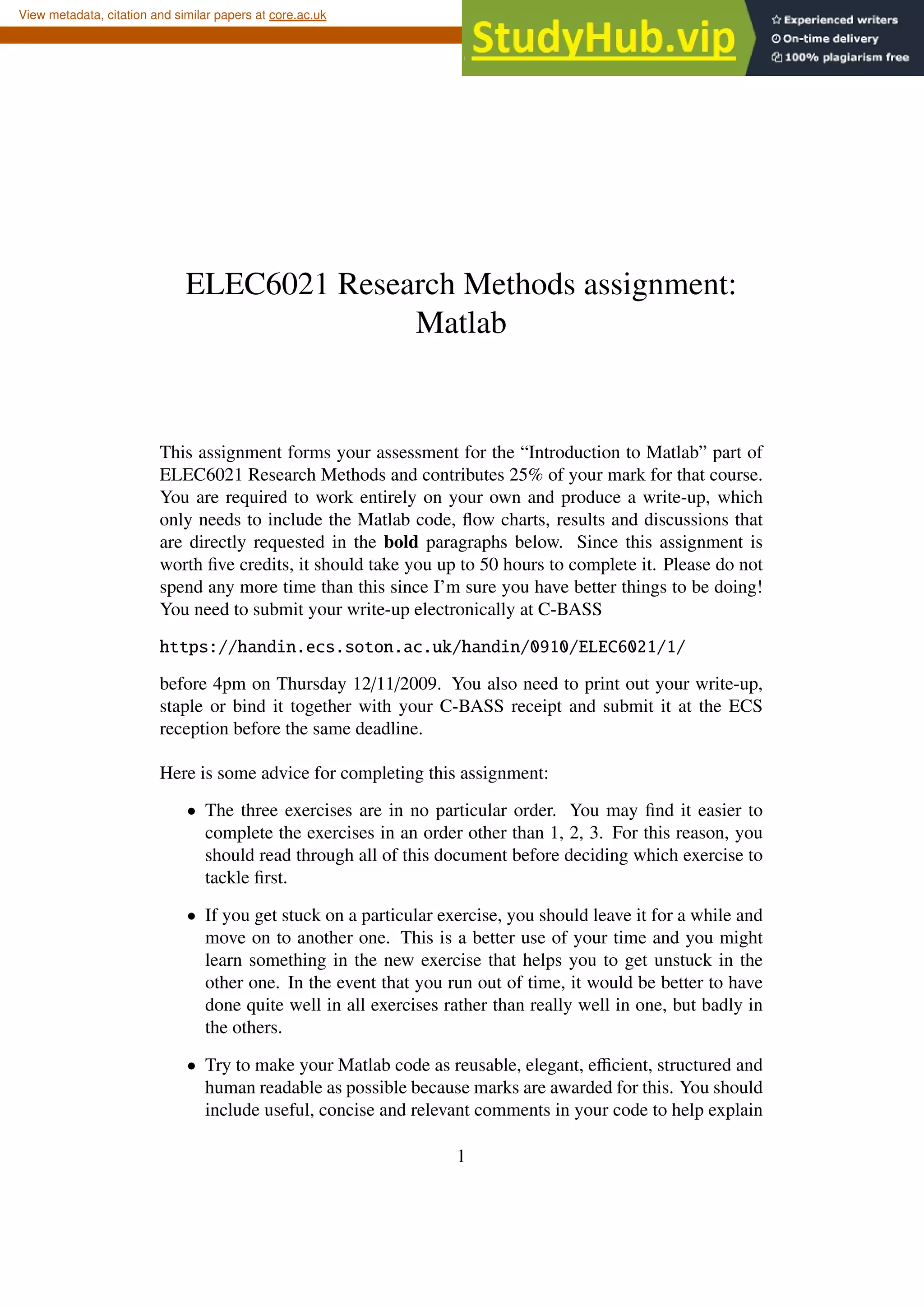
• Figure 3 provides a flow chart that will help you to get started with the
optimise function. This flow chart illustrates the process for determining
the gradient of a function in the vicinity of particular values of its indepen-
dent variables. When drawing your flow chart of the optimise function,
you can use a single box to represent the process illustrated in Figure 3.
• Draw your flow chart of the optimise function on a computer so that it is
easy to move parts around and make changes to it. You should be doing this
in parallel with writing your Matlab code, rather than leaving the flow chart
to the end. You should find that doing things this way will make it easier for
you to break the problem down.
• I found that values of ǫ = 0.0001 and t = 0.0001 work well.
• You will probably find the built-in Matlab functions feval, plot, plot3,
meshgrid, surf and hold to be useful in this exercise.
11](https://image.slidesharecdn.com/assignmentonmatlab-230807142932-1c5cea51/75/Assignment-On-Matlab-11-2048.jpg)

![f and x
j ← j + 1
g
x′
j ← x′
j + ǫ
x′
← x
j ← 1
gj ← f(x′)−f(x)
ǫ
no
yes
j < N
Figure 3: Flow chart for finding the gradient g of the function f in the vicin-
ity of the particular values provided for the N independent variables x =
[x1, x2, x3, . . . , xN]. Here, gj is the jth
element in the 1 by N vector g and ǫ is
a small positive constant.
13](https://image.slidesharecdn.com/assignmentonmatlab-230807142932-1c5cea51/75/Assignment-On-Matlab-13-2048.jpg)


![case, the player chooses the number x of playing cards to take from the top of a
shuffled pack. If more than y number of the selected cards belong to the same suit
then the player gets a score of zero. Otherwise, the player gets a score equal to the
sum of the selected card values, where an ace has a value of 1, a two has a value
of 2, . . . , a jack has a value of 11, a queen has a value of 12 and a king has a value
of 13. For example, in the case where y = 2, the x = 4 cards 5♥ Q♦ 8♥ A♣ would
get a score of 26, since no more than y = 2 of the cards belong to the same suit.
By contrast, the x = 6 cards 5♠ 7♣ 2♦ A♣ J♦ 3♣ would get a score of zero, since
the number of clubs is greater than y = 2.
As with the dice game, draw a flow chart and write a Matlab function for perform-
ing the Monte Carlo simulation of the described card game. The first line of this
Matlab function is required to be as follows.
function cards(x, y, n, file_name)
Here, the arguments of the cards function are used in the same way as those of
the dice function. Again, your code should write the expected scores into a text
file having the format exemplified in Figure 4.
Include listings and flow charts for your two Matlab functions in your write-
up. Also include the text files obtained by the commands
dice(1:20, 1:5, 10000, ’dice.txt’)
cards(1:20, 1:5, 10000, ’cards.txt’)
For both games, identify the optimal value of x for each value of y ∈ [1, 5].
Here is some advice for completing this exercise:
• Note that when rolling x number of dice, the resultant values will all be
independent of each other. However, x number of cards taken from the top
of a shuffled pack will not be independent of each other, since the x selected
cards are guaranteed to have different combinations of suit and value. Your
cards function should efficiently consider this. You can make sure that
your solution is efficient by ensuring that the command cards(52, 13,
1, ’cards.txt’) takes only a moment to run.
hearts, diamonds, clubs and spades. Each card has one of 13 values, namely ace, two, three, four,
five, six, seven, eight, nine, ten, jack, queen and king. No two cards in a pack have the same
combination of suit and value. Therefore, there are four cards having each value in a pack and 13
cards belonging to each suit. For example, the four sixes are 6♥ , 6♦ , 6♣ and 6♠ . Similarly, the
13 diamonds are A♦ , 2♦ , 3♦ , 4♦ , 5♦ , 6♦ , 7♦ , 8♦ , 9♦ , 10♦ , J♦ , Q♦ and K♦ . When a pack is
shuffled, the order of its 52 cards is randomised.
16](https://image.slidesharecdn.com/assignmentonmatlab-230807142932-1c5cea51/75/Assignment-On-Matlab-16-2048.jpg)


This document describes an assignment to write a Matlab function that transforms a matrix A and vector b into upper triangular form to solve simultaneous equations. Students are provided with 6 example matrices A and vectors b to test their function on. They must return the solution vector x, transformed matrix A', and vector b'. The function must include error checking to ensure valid input dimensions.