- The document is a master's thesis report that evaluates the impact on ampacity (current carrying capacity) of power cables according to IEC-60287 when cables are placed in thermally unfavorable conditions.
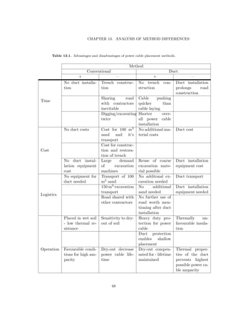
- The report compares a conventional technique of placing cables in cable trenches to a method of placing cables in protective plastic ducts. Comparisons are made regarding ampacity, cost, and technical simplifications.
- Based on the analysis using IEC-60287 models, the results show that placing cables in plastic ducts provides sufficient ampacity for the given circumstances while allowing more flexibility in cable placement logistics compared to cable trenches.


![D.2 Data from probes placed inside the duct, immediately outside the duct
and 2 dm above, surrounded by gravel and stones (material contents
according to 5.3 on page 30). . . . . . . . . . . . . . . . . . . . . . . . . 100
D.3 Data from all probes. . . . . . . . . . . . . . . . . . . . . . . . . . . . . 101
D.4 Moment of heat cable being shut off. Probe on plastic duct surrounded
by sand. . . . . . . . . . . . . . . . . . . . . . . . . . . . . . . . . . . . 102
D.5 Moment of heat cable being shut off. Probe on plastic duct and road
surface. . . . . . . . . . . . . . . . . . . . . . . . . . . . . . . . . . . . . 102
D.6 Moment of heat cable being shut off. Probe inside duct and 2 dm above
surrounded by gravel and stones. . . . . . . . . . . . . . . . . . . . . . . 103
List of Tables
1.1 Reading instructions. . . . . . . . . . . . . . . . . . . . . . . . . . . . . . 6
3.1 Constituents of power cable in figure 3.1. . . . . . . . . . . . . . . . . . 17
6.1 Example table showing time demand. . . . . . . . . . . . . . . . . . . . 34
6.2 Example table describing the material demand in the different methods. 35
6.3 Example table describing logistic demands. . . . . . . . . . . . . . . . . 35
7.1 General conditions. . . . . . . . . . . . . . . . . . . . . . . . . . . . . . . 39
7.2 Common physical quantities for all investigated prerequisites. . . . . . . 42
7.3 Physical quantities for partial dry-out. . . . . . . . . . . . . . . . . . . . 43
7.4 Electric power cable ampacity in two cases. . . . . . . . . . . . . . . . . 44
8.1 Table showing sample from gathered temperature data. . . . . . . . . . 45
9.1 Approximations of phase duration for both power cable placement meth-
ods [18], [19]. See phase description in section 6.1 on page 34. . . . . . . 49
9.2 Material demand in the different cable placement methods [18]. . . . . . 50
9.3 Costs ( [18], [19]). . . . . . . . . . . . . . . . . . . . . . . . . . . . . . . 50
9.4 Actual material cost per km. . . . . . . . . . . . . . . . . . . . . . . . . 51
9.5 Logistic demands [6], [18], [20], [16]. . . . . . . . . . . . . . . . . . . . . 51
10.1 Temperature vs. ampacity. . . . . . . . . . . . . . . . . . . . . . . . . . 57
11.1 Mean temperatures with heat cable on and off. . . . . . . . . . . . . . . 61
2](https://image.slidesharecdn.com/ampacityaccordingtoiec-60287-191019201759/85/Ampacity-according-to-iec-60287-14-320.jpg)

![CHAPTER 1. INTRODUCTION
and social planning."2
"The Electromagnetic Engineering lab (ETK) is one out of the twelve labs in the
School of Electrical Engineering at the Royal Institute of Technology. It was formed
at the end of 2005 by merging of the divisions of Electrotechnical design (EEK) and
Electromagnetic Theory (TET). In 2009, the Electromagnetic Compatibility (EMC)
group at Uppsala University was moved to this division."3
The second supervisor is Assoc. Prof. Hans Edin at the department of Electromag-
netic Engineering, School of Electrical Engineering. He is currently leader of the
high voltage engineering and insulation diagnostic group.
1.2 Purpose
The purpose of this master thesis is to investigate whether suggested changes to con-
ventional cable laying techniques can contribute to the overall optimization process.
Useful contributions are: acceptable ampacity level of power cable, lower installa-
tion costs, greater flexibility in project implementation, higher work place safety,
minimization of simultaneous contractors on site, greater maintenance flexibility
and shorter construction time.
1.3 Goals
The goals of this master thesis are divided into three sections: assignment, problem
formulation and project question.
1.3.1 Assignment
In this masters’ degree project, these are the key assignments:
Evaluate the suggested method for power cable placement according to IEC-
60287.
Based on empiric data, evaluate the model describing the material surrounding
the power cable.
1.3.2 Problem formulation
According to the project description [12], six questions states the problem.
Does the suggested new method in power cable placement allow greater flex-
ibility in time planning?
2
About KTH, www.kth.se, 2011-06-15
3
ETK, www.etk.ee.kth.se, 2011-06-06
8](https://image.slidesharecdn.com/ampacityaccordingtoiec-60287-191019201759/85/Ampacity-according-to-iec-60287-20-320.jpg)

![CHAPTER 2. METHOD
periment implementations are described. Economic investigations according to the
economic review are presented.
2.4 Analysis
Analysis is the single most important part of the report. The analysis is based
entirely on results from data gathering and validated only through IEC 60287 (
[1], [2], [3]) and in acceptance and ideas from experienced participants (project
supervisors et al).
After performing the analysis, conclusions are presented in the conclusions section.
The most important purpose of the conclusions section is to answer the questions
from the project goals (in section 1.3 on page 8).
2.5 Presentation
The last stage of the master thesis is to orally present the work that has been
performed. Naturally the report is an important part of the presentation, but even
more important are the views and ideas of the author and feedback from supervisors
and others involved. Suggestions on future work in the area will also be presented.
The oral presentation is open and can be visited by anyone with an interest in the
subject.
12](https://image.slidesharecdn.com/ampacityaccordingtoiec-60287-191019201759/85/Ampacity-according-to-iec-60287-24-320.jpg)


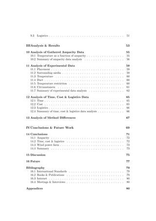
![Chapter 3
General Theory on Electric Power
Transfer in Wind Power Farms
Large wind power plants produce electric power in the vicinity of 1.5 MW up to 5
MW (or in some cases more1). Wind power plants deliver their produced power to
a transformer. Before feeding the electricity into the public grid, the transformer
converts the electricity from the generated voltage to a more suitable high voltage
(Page 211 in Developing wind power projects, Wizelius, 2007, [10]).
The power cable that connects the wind power plant with the transformer has to
have a power cable ampacity large enough to be able to handle the power produced
in the wind power plant. Dimensioning the power cable is done according to the
power output of the wind power plant. However, due to increased costs in increased
cable dimension, the cable should have an ampacity that is large enough, but not
too large.
Figure 3.1 and 3.3 describes the geometry of the power cable AXKJ-F 3x95/25.
Figure 3.1 shows all constituent parts of the cable and in table 3.1 all parts are
described. Figure 3.3 shows the setup with the power cable placed in a protective
duct. Figure 3.2 shows a 3D view [11] of the cutaway view in figure 3.1.
3.1 Thermal stress
According to the Arrhenius equation, at room temperature chemical reactions dou-
bles their reaction rate for every 10 °C increase in temperature [9].
Due to the change in reaction rate, described in the Arrhenius equation, power ca-
bles deteriorate/age faster under thermal stress. Hence, thermal stress should be
avoided to benefit expected lifetime for a power cable.
1
E.g. the Enercon E-126 has a rated power of 7.5 MW.
15](https://image.slidesharecdn.com/ampacityaccordingtoiec-60287-191019201759/85/Ampacity-according-to-iec-60287-27-320.jpg)
![CHAPTER 3. GENERAL THEORY ON ELECTRIC POWER TRANSFER IN WIND
POWER FARMS
Screen
Serving PP C paper
Semicon
Semicon
X
X
Semicon
Semicon
Semicon
Cond.
Cond.
Cond.
Figure 3.1. Geometry of the Power Cable, 2D Profile
Figure 3.2. Threedimensional view of three phase power cable.
One of the reasons to why a cable is exposed to thermal stress is it’s geometry and
construction. Cables covered with protective plastics or metals isolates and pre-
serves heat better than cables without these protective layers (thermal resistance
in equation 3.1 calculated according to IEC-60287-2-1 [2]). A power cable system
(power cable, cable protection and surrounding medium) that preserves heat suffers
from increased temperature and is hence exposed to thermal stress.
The electrical resistance of the power cable increase with temperature according to
equation 4.5 from IEC-60287-1-1 [1]. An increase in electrical resistance leads to an
increased loss in electric power (see equation 5.1) in the form of heat.
Power cables placed in ground are not only affected, in terms of heat isolation, by
16](https://image.slidesharecdn.com/ampacityaccordingtoiec-60287-191019201759/85/Ampacity-according-to-iec-60287-28-320.jpg)
![3.2. THERMAL RESISTANCE
Table 3.1. Constituents of power cable in figure 3.1.
Serving non-extruded layer or assembly of non-extruded layers applied to the
exterior of a cable 2, but can also be called outer sheath;
Screen 25 mm2 Copper screen;
PP Polypropylene. Belongs to the group thermoplastic polymers. Keeps
the screen fixed during manufacturing;
C paper Carbon paper. Plastic material covered in carbon particles. Additional
screen;
Semicon Outer and inner semi conductor;
X Cross-linked polyethylene used for isolation and protection;
Cond. 95 mm2 aluminium conductor;
protective plastic and/or metallic layers. Surrounding medium such as soil, sand,
gravel, water, mud or air have a profound effect on heat isolation properties of the
system. This will be closer explained in section 3.2.
3.2 Thermal resistance
Heat produced in any system is transferred via mediums surrounding the heat
source. Depending on medium properties the heat transfer ability differs between
different mediums. Heat transfer can be classified in different groups such as convec-
tion, conduction and radiation (see section 1.2 in Rating of Electric Power Cables...
G J Anders, 2005, [4]). In figure 3.4 heat transfer can be seen as radiation and
conduction. Due to the thermal properties of surrounding mediums, the thermal
resistance of the system does not only rely on the construction of the power cable
(see equation 3.1), but all constituent layers add thermal resistance and even the
surrounding soil/sand is important to account for (see equation 3.2 below).
To calculate the ampacity of a power cable according to IEC-60287 many properties
of the cable needs clarification, simplification and structuring. This is done in sec-
tion 4. The thermal resistance of the power cable is one of the constituents needed
in the international standard to calculate the ampacity.
The thermal resistance of a power cable can according to IEC-60287-2-1 [2] be
described as:
T = T1 + T2 + T3 (3.1)
where
T1 is the thermal resistance between one conductor and sheath (see cable de-
scription in section 3.1) [Km/W];
T2 is the thermal resistance between sheath and armour [Km/W];
17](https://image.slidesharecdn.com/ampacityaccordingtoiec-60287-191019201759/85/Ampacity-according-to-iec-60287-29-320.jpg)
![CHAPTER 3. GENERAL THEORY ON ELECTRIC POWER TRANSFER IN WIND
POWER FARMS
1 cm2
Figure 3.3. Geometry of the power cable placed in a plastic duct (cross section)
T3 is the thermal resistance of outer covering/serving [Km/W];
Thermal resistances distinguishes the two methods where the power cables are either
placed in a trench or in a duct. The construction of the power cable is the same in
both cases. The only thing that differentiates between them is the outer thermal
resistance T4. One power cable is placed directly in wet soil, the other in an air
filled plastic duct. In the air filled plastic duct the thermal resistance is higher than
when soil and gravel surrounds the power cable (Tsoil<Tair [1]). Furthermore, the
medium around the power cable and outside the plastic duct have different thermal
properties. Since the power cable placed in the duct is better protected than the
cable in the trench more coarse soil/gravel can be used. In the method where a
duct is used, the material surrounding the system is assumed to have the same or
higher thermal resistance than sand or soil. Hence the lowest calculated ampacity is
chosen in chapter 10 since a decrease in current carrying capacity can be expected
(also found in chapter 10) compared to conventional power cable placement. T4 is
18](https://image.slidesharecdn.com/ampacityaccordingtoiec-60287-191019201759/85/Ampacity-according-to-iec-60287-30-320.jpg)
![Chapter 4
Theory on Calculating Ampacity
According to IEC-60287
Road surface
Conditions:
θa=20°C ambient soil temperature;
θ=90°C power cable core temperature;
ρw=1 Km/W thermal resistivity of wet soil;
ρd=3 Km/W thermal resistivity of dry soil;
L=1 m placement depth.
Three phase power cable Plastic duct
=64 mm =110 mm
L
Figure 4.1. Fundamental assumptions such as power cable burial depth etc.
This chapter contains clarifications regarding the use of the international stan-
dard IEC-60287. All sections are presented according to the standard documents
IEC-60287-1-1 [1], IEC-60287-2-1 [2] and IEC-60287-3-2 [3], with comments where
simplifications or alterations have been performed. IEC-60287 is used to establish
the permissible current rating (ampacity) of a power cable. The standard contains
formulas for calculating losses (ac resistance and dielectric losses), loss factors for
power cable constituents (reinforcements etc.) and thermal resistances throughout
the entire system (power cable, protective covering and surrounding medium). A
full description of prerequisites is found in Appendix A.
21](https://image.slidesharecdn.com/ampacityaccordingtoiec-60287-191019201759/85/Ampacity-according-to-iec-60287-33-320.jpg)
![CHAPTER 4. THEORY ON CALCULATING AMPACITY ACCORDING TO
IEC-60287
The scope of IEC-60287 according to IEC [1]:
"... IEC-60287 is applicable to the conditions of steady-state operation of cables
at all alternating voltages, and direct voltages up to 5 kV, buried directly in the
ground, in ducts, troughs or in steel pipes, both with and without partial drying-out
of the soil, as well as cables in air. The term "steady state" is intended to mean a
continuous constant current (100 % load factor) just sufficient to produce asymp-
totically the maximum conductor temperature, the surrounding ambient conditions
being assumed constant."
4.1 Ampacity
The permissible current rating of electric power cables will throughout this master
thesis be referred to as ampacity.
Since the ampacity of the power cable is calculated for real conditions, both partial
dry-out (section 4.1.2) of the surrounding medium and no dry-out at all (section
4.1.1) is considered. Due to the fact that both scenarios can occur and the least
favourable (lowest ampacity) should be counted for, the lowest of the two ampaci-
ties is chosen. In this section the main parts of IEC-60287 are described.
In IEC-60287-1-1 [1] the ampacity of an AC cable is derived from the expression for
the temperature rise of the cable conductor above ambient temperature:
∆θ = (I2
R +
1
2
Wd)T1 + [I2
R(1 + λ1) + Wd]nT2 + [I2
R(1 + λ1 + λ2) + Wd]n(T3 + T4)
(4.1)
All constituents in equation 4.1 are explained in the following sections. From equa-
tion 4.1 the ampacity (I in the equation) can be derived in different ways to adapt
to different circumstances. Below, two different ways of using equation 4.1 are
presented.
4.1.1 Buried cables where drying-out of the soil does not occur
A power cable buried in an environment where the soil does not become dry. A con-
tinuous contribution of dampness can be expected. Wet surroundings have different
properties than dry (see section 3.1). The permissible current rating is obtained
from 4.1 according to IEC 60287-1-1 [1] as follows:
I =
∆θ − Wd[0.5T1 + n(T2 + T3 + T4)]
R[T1 + n(1 + λ1)T2 + n(1 + λ1 + λ2)(T3 + T4)]
0.5
(4.2)
22](https://image.slidesharecdn.com/ampacityaccordingtoiec-60287-191019201759/85/Ampacity-according-to-iec-60287-34-320.jpg)
![4.2. CALCULATION OF LOSSES
4.1.2 Buried cables where partial drying-out of the soil occurs
In areas where dry-out of surrounding medium can be expected, the ampacity cal-
culations must be adapted. The permissible current rating is obtained from 4.1
according to IEC 60287-1-1 [1] as follows:
I =
∆θ − Wd[0.5T1 + n(T2 + T3 + vT4)] + (v − 1)∆θx
R[T1 + n(1 + λ1)T2 + n(1 + λ1 + λ2)(T3 + vT4)]
0.5
(4.3)
4.2 Calculation of losses
The heat produced in a power cable is 100 % losses. Ideally, all power is transferred
as electricity and nothing is lost to other forms of energy. In reality, the system have
losses that heats the conductor and affects it’s surroundings. This section describes
the losses and how it affects the ampacity.
4.2.1 AC resistance of conductor
The AC resistance of a conductor consist of the DC resistance, the skin effect and the
proximity effect. Working at maximum operating temperature, the AC resistance
(per unit length), according to IEC-60287-1-1 section 2.1, is given by:
R = R (1 + ys + yp) (4.4)
DC resistance of conductor
R = R0[1 + α20(θ − 20)] (4.5)
where
R0 is the d.c. resistance of the conductor at 20 °C [Ω/m];
α20 is the constant mass temperature coefficient for aluminium at 20 °C per
Kelvin;
θ is the maximum operating temperature in °C.
Skin effect factor ys
At rising frequencies the skin effect effectively limits the cross-sectional area of the
conductor [7]. Due to concentration of currents at the surface, the resistance of
the conductor increases and hence the ampacity is decreased. The skin effect is a
phenomenon that depends on frequency and therefore causes AC resistance to be
higher than DC resistance (page 20 in Practical Transformer Handbook, Irving M
Gottlieb, 1998, [7]).
23](https://image.slidesharecdn.com/ampacityaccordingtoiec-60287-191019201759/85/Ampacity-according-to-iec-60287-35-320.jpg)
![CHAPTER 4. THEORY ON CALCULATING AMPACITY ACCORDING TO
IEC-60287
The skin effect factor ys is given by:
ys =
x4
s
192 + 0.8 · x4
s
(4.6)
where
x2
s =
8πf
R
· 10−7
· ks (4.7)
f is the supply frequency in hertz.
ks coefficient according to IEC–60287 [1] table 2. Depending on conductor type
(e.g. helical) and strand impregnation.
Proximity effect factor yp (for three-core cables)
When circulating currents occur due to alternating magnetic flux caused by current
flows in nearby conductor(s), the resistance of the conductor is increased (page 395
in Power System Engineering, R K Rajput, 2006, [8]). This is what is called prox-
imity effect.
Three phase power cables having three conductors gives a proximity effect factor,
according to IEC-60287-1-1, of:
yp =
x4
p
192 + 0.8x4
p
dc
s
2
0.312 ·
dc
s
2
+
1.18
x4
p
192+0.8x4
p
+ 0.27
(4.8)
where
x2
p =
8πf
R
· 10−7
· kp (4.9)
dc is the diameter of conductor [mm];
s is the distance between conductor axes [mm];
kp coefficient according to IEC–60287 [1] table 2. Depending on conductor type
(e.g. helical) and strand impregnation.
24](https://image.slidesharecdn.com/ampacityaccordingtoiec-60287-191019201759/85/Ampacity-according-to-iec-60287-36-320.jpg)
![4.2. CALCULATION OF LOSSES
4.2.2 Dielectric losses
Cables investigated in this master thesis are insulated with cross-linked polyethy-
lene. This type of dielectric medium, when subject to alternating currents, is run
through by charging currents (page 109, Rating of Electric Power Cables:..., George
J Anders, 1997, [5]). The work required to move electrons back and forth in the
dielectric at the same frequency as the alternating current, generates heat and is a
loss of power - this is the dielectric loss [5].
The dielectric loss per unit length in each phase is given by:
Wd = ωCU2
0 tan δ [W/m] (4.10)
where
ω = 2πf;
U0 is the voltage to earth [V ].
The capacitance for circular conductors is given by:
C ≈
ε
18 ln Di
dc
· 10−9
[F/m] (4.11)
where
ε is the relative permittivity of the insulation;
Di is the external diameter of the insulation (excluding screen) [mm];
dc is the diameter of conductor, including screen [mm].
4.2.3 Loss factor for screen
The power loss in the screen ( λ1 ), according to IEC-60287-1-1 section 2.2, consists
of losses caused by circulating currents ( λ1 ) and eddy currents ( λ1 ), thus:
λ1 = λ1 + λ1 (4.12)
where
λ1 =
RS
R
1
1 + RS
X
2 (4.13)
X = 2ω · 10−7
ln
2s
d
(4.14)
where
25](https://image.slidesharecdn.com/ampacityaccordingtoiec-60287-191019201759/85/Ampacity-according-to-iec-60287-37-320.jpg)
![CHAPTER 4. THEORY ON CALCULATING AMPACITY ACCORDING TO
IEC-60287
X is the reactance per unit length of sheath or screen per unit length of cable
[Ω/m];
ω = 2πf [rad/s];
s is the distance between conductor axes in the electrical section being con-
sidered [mm];
d is the mean diameter of the sheath [mm];
λ1 = 0. The eddy-current loss is ignored according to IEC 60287-1-1 section
2.3.1 [1].
Rs is the resistance of the screen per unit length of cable at its maximum operating
temperature [Ω/m].
RS = RS0 [1 + α20(θSC − 20)] [Ω/m] (4.15)
where
RS0 is the resistance of the cable screen at 20 °C [Ω/m].
4.3 Thermal resistance T
As described in section 3.2 thermal resistance occurs wherever there are mediums
limiting heat transfer. Following section explains important parts in calculating
what the constituents of a power cable adds in term of thermal resistance.
4.3.1 Thermal resistance of constituent parts of an electric power
cable, T1, T2, T3
According to IEC-60287-2-1 [2], the thermal resistance, T, is:
T = T1 + T2 + T3
Thermal resistance between one conductor and sheath T1
For screened cables with circular conductors the thermal resistance T1 is [2]:
T1 =
ρT
2π
G (4.16)
where
G is the geometric factor according to IEC60287 [2];
ρT is the thermal resistivity of insulation [Km/W];
26](https://image.slidesharecdn.com/ampacityaccordingtoiec-60287-191019201759/85/Ampacity-according-to-iec-60287-38-320.jpg)
![4.3. THERMAL RESISTANCE T
Thermal resistance between sheath and armour T2
The investigated power cable does not contain armour nor metallic sheath. Hence
T2 is not considered.
Thermal resistance of outer covering (serving) T3
T3 =
ρT
2π
· ln 1 +
2t3
Da
(4.17)
where
t3 is the thickness of serving [mm];
Da is the external diameter of the armour [mm];
4.3.2 External thermal resistance T4
The external thermal resistance of a cable in a duct consists of three parts:
T4 is the thermal resistance of the air space between the cable surface and
duct’s internal surface;
T4 is the thermal resistance of the duct itself;
T4 is the external thermal resistance of the duct (sand, soil, gravel, etc.).
T4 = T4 + T4 + T4 (4.18)
Thermal resistance between cable and duct T4
T4 =
U
1 + 0.1(V + Y θm)De
(4.19)
where
U, V and Y are material constants defined in IEC-60287 [2] table 4.
De is the external diameter of the cable [mm];
θm is the mean temperature of the medium filling the space between
cable and duct. [°C];
27](https://image.slidesharecdn.com/ampacityaccordingtoiec-60287-191019201759/85/Ampacity-according-to-iec-60287-39-320.jpg)
![CHAPTER 4. THEORY ON CALCULATING AMPACITY ACCORDING TO
IEC-60287
Thermal resistance of the duct T4
T4 =
ρT
2π
· ln
D0
Dd
(4.20)
where
D0 is the outside diameter of the duct [mm];
Dd is the inside diameter of the duct [mm];
ρT is the thermal resistivity of duct material [Km/W]
External thermal resistance of the duct T4
T4 =
1
2π
ρsoil · ln (2u) (4.21)
where
ρsoil is the thermal resistivity of earth around bank [Km/W];
u = 2L
D0
, L is the depth of the laying to centre of duct [mm];
28](https://image.slidesharecdn.com/ampacityaccordingtoiec-60287-191019201759/85/Ampacity-according-to-iec-60287-40-320.jpg)
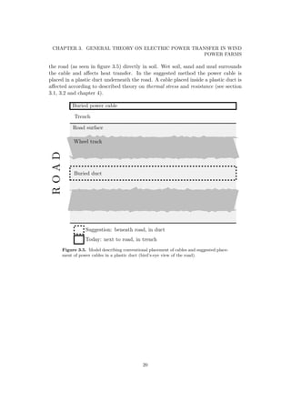
![Chapter 5
Theory on Experiment Implementation
The current ampacity of a power cable is affected by surrounding mediums and
the mediums’ thermal resistances (IEC-60287-1-1 section 1.4.1.1 [1] and Rating of
Electric Power Cables section 1.3.1, George J Anders, 2005 [4]). This makes the
thermal properties of the surroundings interesting when rating power cables.
To find the thermal properties of the surroundings an on-site experiment has been
performed. Temperature sensors were placed at different locations in and around
dug down cable ducts. A heat cable was installed in the duct and the sensors were
used to log how heat spread through the system. This section describes the purpose
and set-up of the experiment.
5.1 Experiment purpose
The purposes of performing this experiment are:
• Find temperature transients regarding heat up and cool down1 of the power
cable system2.
• Observe how heat spreads through system components.
• Investigate damages on ducts placed beneath road surface.
• Gather views on how the new set-up3 is looked upon.
• Find inaccuracies in measurement equipment.
5.2 Equipment
• Plastic ducts (Polyethylene), 10 m long
1
How quickly is a temperature equilibrium reached at power up and power down?
2
Power cable, duct and surrounding material
3
Power cable placed beneath the road surface instead of next to the road.
29](https://image.slidesharecdn.com/ampacityaccordingtoiec-60287-191019201759/85/Ampacity-according-to-iec-60287-41-320.jpg)
![CHAPTER 5. THEORY ON EXPERIMENT IMPLEMENTATION
Figure 5.1. Data logger used to store temperature data (© Gemini Dataloggers UK,
2011).
• Heat cable, 10 m long, 10 [W/m], see calculations in section 5.3
• 4 data loggers (see figure 5.1) for data storage, storage capacity=16000 values
(≈ 1 temperature sample every 5 minutes for 55 days).
• 6 temperature sensor probes (1.5 m, waterproof flexible thermistor probe)
• Joint foam (used to seal the duct halfway through to avoid heat leakage be-
tween measurement points)
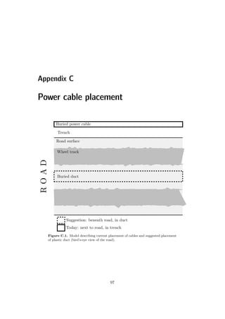
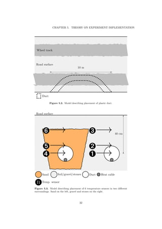
5.3 Experiment set-up
3 sets of respectively 8 meters plastic ducts were placed beneath the road surface at
an emerging wind power park. The ducts were placed in the road before any heavy
transports had begun. All ducts were then left in the road during construction of
3 wind power plants. When the constructions was finished the ducts were dug up
and controlled for damages.
At the same time when two of these ducts were dug up, the third duct was left in
the road and a heat cable and temperature sensors were installed. Figure 5.2 shows
the duct in relation to the road and where the wheel tracks are located. The heat
cable was used to simulate the presence of a real power cable working at maximum
load. To accurately dimension the heat cable (Pheatcable ≈ Ploss) an approximation
of the power cable ampacity, according to the following equation, is demanded:
30](https://image.slidesharecdn.com/ampacityaccordingtoiec-60287-191019201759/85/Ampacity-according-to-iec-60287-42-320.jpg)
![5.3. EXPERIMENT SET-UP
Ploss = I2
· R (5.1)
where
I = 230 [A], the maximum load of the power cable with conductor at maximum
operating temperature θ = 90 °C;
R = 0.320
1000 · (1 + α20(θ − 20)) = 0.000381445 [Ω/m], the dc resistance of the
conductor per meter at max operating temperature according to IEC60287-
1-1 [1].
which gives
Ploss = 2302
· 0.000381445 ≈ 20.2 [W/m]
This means that the heat cable, used to simulate the power cable, should be dimen-
sioned to produce 20.2 W/m.
Figure 5.3 on page 32 shows the temperature sensor set-up. One side of the duct
was covered in coarse sand4 and the other side was covered with material directly
from the road (very coarse mix of sand, sandy till5, mud and stones).
A small hole was drilled on top of the duct and sensors placed according to in-
dicators 4 and 1 in figure 5.3 on page 32. Indicator 2 and 5 in figure 5.3 shows
the placement of sensors immediately outside the duct. The sensors placed furthest
away from the heat cable and closest to the road surface are indicators 3 and 6.
As mentioned above, joint foam was used to seal the two ends from each other and
also to keep the heat cable fixed during the 12 days of data gathering. Three of the
data loggers can handle input from 2 sensors each. The fourth has 1 data channel.
On the ninth day the heat cable was shut off and the system was left to cool.
After 12 days of continuous measurement the data loggers were collected and the
data extracted.
5.3.1 Duct
There were two types of ducts placed in the road. The duct used in this experiment
set-up is called SRS110 and is a reinforced 8 mm thick PVC duct. The other duct
was a corrugated, but not as sturdy, type called SRN110. Two ducts (one of each
type) were placed on a depth of 30 cm and one SRS110 was placed at a depth of 40
cm.
4
According to ISO 14688-1:2002, sand with a grain diameter of between 0.5 mm-1 mm
5
Unsorted glacial sediment mixed with sand. Swedish: ’sandig morän’.
31](https://image.slidesharecdn.com/ampacityaccordingtoiec-60287-191019201759/85/Ampacity-according-to-iec-60287-43-320.jpg)
![Chapter 6
Theory on Time, Cost & Logistics
As stated in section 1.2 and 1.3 Statkraft is interested in finding advantages and
disadvantages in different techniques for power cable placement. Areas of interest
are economy, safety and planning flexibility . Are there benefits with other methods
for electric power cable placement in comparison to methods used today? This
section will foremost be based on views from Statkraft employees and contractors
working with projects connected to the purpose and goals of this master thesis.
Data has been gathered through interviews, collaborations, questionnaires, email
conversations and phone calls during the project.
6.1 Time
Time is of the essence when constructing a wind power park. There are many phases
of the project that affects the time plan and three examples of important parts1 are
(Chapter 19 in Developing Wind Power Projects, T Wizelius (2008), [10]):
Road finished When the road, connecting the wind power plant sites with
each other and the closest main road, is finished, the con-
struction of the power plant foundation can be initiated;
Commissioning Not until the wind power plant delivers electricity to the grid,
the cost for the wind power plant starts paying back;
Flexibility Coordination of contractors working on the same site to pre-
vent cross-planning2 and accidents. What is sought is flexi-
bility in phase implementation and reaching a shorter time of
construction.
The table below is used to roughly approximate time consumption in the two meth-
ods (existing method and suggested method). All phases defined as "-" are phases
identical for the two methods or phases not affected by cable placement method.
1
Reaching an identifiable, important step in a project.
2
E.g. contractors working at the same place at the same time.
33](https://image.slidesharecdn.com/ampacityaccordingtoiec-60287-191019201759/85/Ampacity-according-to-iec-60287-45-320.jpg)
![CHAPTER 6. THEORY ON TIME, COST & LOGISTICS
The phases marked "-" will not be considered when comparing the cable placement
methods.
Following list describes the table content.
Lumbering Removal of trees and vegetation above ground level.
Excavation, blasting Removal of stubs, rocks and other irregularities below
ground level. An area the width of the road, and desired
depth (≈ 1 m), is cleared for the road construction.
Duct installation The plastic duct is installed in the bottom of the road-
to-be. This part includes the difference in time between
the two different cable placement methods.
Road construction A road is constructed according to a layer-on-layer prin-
ciple with different mediums on different depths (method
similar to Swedish transport administration , publica-
tion 2008:78, page 5 [15]). Differences in road construc-
tion are included in duct installation.
Trench construction Digging a trench next to the road where the power cable
will be placed.
Cable installation The electric power cable is placed either in a trench or in
a plastic duct underneath the road surface. In the trench
scenario, the power cable is winded from the cable reel
directly into the trench. When a plastic duct is used,
the power cable is pushed through the duct.
Electric installation Connecting the power cables to the wind power plant,
the transformer and the power grid.
Table 6.1. Example table showing time demand.
Time demand [hours/1000 m]
Phase Existing method Suggested method
Lumbering - -
Excavation, blasting - -
Duct installation
Road construction - -
Trench construction
Cable installation
Electric installation - -
Σ
34](https://image.slidesharecdn.com/ampacityaccordingtoiec-60287-191019201759/85/Ampacity-according-to-iec-60287-46-320.jpg)
![6.2. COST
6.2 Cost
Material and service costs are the major parts of the total project cost. Both
material demand and service need3 are included in the project plan, but only the
material demand is unlikely to change during the project4 while the need for services
is more flexible. Man hours for contractors are not included in table 6.2 since they
are accounted for in table 9.1. The cable pushing equipment mentioned in table 6.2
are the machines required to push/pull the power cable into the plastic duct. One
machine is placed at the duct entrance where it pushes the power cable. The second
machine is placed at the exit of the duct where the cable is pulled.
Table 6.2. Example table describing the material demand in the different methods.
Material demand /1000 m
Item Existing method Suggested method
Sand Volume m3 Volume m3
Plastic duct Length m Length m
Cable pusher Pcs Pcs
6.3 Logistics
What are the logistic demands and profits of the different power cable placments?
Table 6.3. Example table describing logistic demands.
Service demand /1000 m
Service Existing method Suggested method
Excavation removal Volume m3 Volume m3
Sand transports Volume m3 Volume m3
Power cable transport Length m, weight
kg
Length m, weight
kg
Duct transport Length m, weight
kg
Length m, weight
kg
3
Excavation, transports, duct installation, etc.
4
According to Kjell Gustafsson [20] and Urban Blom [21]
35](https://image.slidesharecdn.com/ampacityaccordingtoiec-60287-191019201759/85/Ampacity-according-to-iec-60287-47-320.jpg)


![CHAPTER 7. GATHERING AND CALCULATION OF AMPACITY DATA
1. Buried cables where drying-out of the soil does not occur
2. Buried cables where partial drying-out of the soil occurs
7.2 Calculation of losses
See chapter 4 for further description.
7.2.1 AC resistance of conductor
R = R (1 + ys + yp) (7.1)
DC resistance of conductor
R = R0[1+α20(θ−20)] = 0.00029752·[1+4.03·10−3
(90−20)] = 0.00038144 Ω (7.2)
Skin effect factor ys
ys =
x4
s
192 + 0.8 · x4
s
=
0.573974
192 + 0.573974
= 0.00056501 (7.3)
xs =
8πf
R
· 10−7 · ks = {ks = 1} =
8π50
0.00038144
· 10−7 = 0.57397
Proximity effect factor yp (for three-core cables)
The proximity effect factor is given by:
yp =
x4
p
192 + 0.8x4
p
dc
s
2
0.312 ·
dc
s
2
+
1.18
x4
p
192+0.8x4
p
+ 0.27
= ... = 0.00025545
(7.4)
xp =
8πf
R
· 10−7 · kp = {kp = 0.8} =
8π50
0.00038144
0.8 · 10−7 = 0.26355
→ R = R (1 + ys + yp) = 0.00038144 · (1 + 0.00056501 + 0.00025545) Ω =
0.0038175 Ω
The impact from skin- and proximity effect on the AC resistance is less than 1 .
40](https://image.slidesharecdn.com/ampacityaccordingtoiec-60287-191019201759/85/Ampacity-according-to-iec-60287-52-320.jpg)
![7.3. THERMAL RESISTANCE T
7.2.2 Dielectric losses
The dielectric loss per unit length in each phase is given by:
Wd = ωCU2
0 tan δ = 2π50 · 0.16392 · 10−9
(
36
√
3
· 103
)2
· 0.004 W/m = 0.088987 W/m
(7.5)
7.2.3 Loss factor (λ1) for screen
λ1 = λ1 + λ1 (7.6)
λ1 =
RS
R
1
1 + RS
X
2 =
0.000856394952
0.0038175
1
1 + 0.000856394952
5.275·10−6
2 = 8.798 · 10−5
The eddy-current loss λ1 is ignored according to IEC 60287-1-1 section
2.3.1 [1].
λ1 = λ1 + λ1 = 8.798 · 10−5
+ 0 = 8.798 · 10−5
7.3 Thermal resistance T
See section 4.3 for extended explanation of how the thermal resistance T is consid-
ered.
T = T1 + T2 + T3 + T4
7.3.1 Internal thermal resistances, T1, T2 and T3
Thermal resistance between one conductor and sheath T1
T1 =
ρT,PEX
2π
G =
3.5
2π
1.63 Km/W ≈ 0.91 Km/W (7.7)
G is a geometric factor based on the diameter of the conductor, thickness of insula-
tion between conductors and thickness of insulation between conductor and sheath.
See IEC-60287 [2] figure 3 for details.
Thermal resistance between sheath and armour T2
AXKJ-F 3x95/25 does not contain armour nor metallic sheath. Hence T2 is not
considered.
T2 = 0 (7.8)
41](https://image.slidesharecdn.com/ampacityaccordingtoiec-60287-191019201759/85/Ampacity-according-to-iec-60287-53-320.jpg)
![7.5. AMPACITY IN TWO CASES
7.4.1 Buried cables where drying-out of the soil does not occur
As declared in chapter 4 the ampacity can be calculated according to:
I =
∆θ − Wd[0.5T1 + n(T2 + T3 + T4)]
R[T1 + n(1 + λ1)T2 + n(1 + λ1 + λ2)(T3 + T4)]
0.5
(7.15)
7.4.2 Buried cables where partial drying-out of the soil occurs
The permissible current rating is obtained from 4.1 according to [1] as follows:
I =
∆θ − Wd[0.5T1 + n(T2 + T3 + vT4)] + (v − 1)∆θx
R[T1 + n(1 + λ1)T2 + n(1 + λ1 + λ2)(T3 + vT4)]
0.5
[A] (7.16)
Table 7.3. Physical quantities for partial dry-out.
Physical
quantity
Partial dry-out
ρd 3 Km/W
ρw 1 Km/W
v 3
θx 50 °C
θa 20 °C
∆θx 30 K
ρd, ρw is the thermal resistivity of the dry/moist soil;
v =ρd/ρw, the ratio of the thermal resistivities of the dry and moist soil
zones;
θx is the critical temperature rise of the soil and temperature of the boundary
between dry and moist zones;
∆θx =θx − θa, the critical temperature rise of the soil. θa is the ambient
temperature of the soil.
7.5 Ampacity in two cases
With the power cable placed in a plastic duct at the depth of 1 m, conductor
temperature of 90°C and an ambient temperature of 20°C the following data is
gathered.
43](https://image.slidesharecdn.com/ampacityaccordingtoiec-60287-191019201759/85/Ampacity-according-to-iec-60287-55-320.jpg)
![CHAPTER 7. GATHERING AND CALCULATION OF AMPACITY DATA
Table 7.4. Electric power cable ampacity in two cases.
Specification Ampacity [A]
No dry-out 205
Partial dry-out 180
44](https://image.slidesharecdn.com/ampacityaccordingtoiec-60287-191019201759/85/Ampacity-according-to-iec-60287-56-320.jpg)
![Chapter 8
Experiment Data
8.1 Data logg
When all data loggers were collected from the measurement site, the data was
downloaded to a computer in the format seen in table 8.1. The data in table 8.1 is
unedited, unfiltered and has not been corrected in terms of errors, hence the rough
usage of significant figures.
Table 8.1. Table showing sample from gathered temperature data.
Gathered data
Date Time Sensor 1 temperature [°C] Sensor 2 temperature [°C]
2011-05-17 16:34:00.000 16.9956 14.2653
2011-05-17 16:39:00.000 16.9999 14.2610
2011-05-17 16:44:00.000 17.0142 14.2639
2011-05-17 16:49:00.000 17.0286 14.2653
2011-05-17 16:54:00.000 17.0257 14.2668
2011-05-17 16:59:00.000 17.0329 14.2682
2011-05-17 17:04:00.000 17.0344 14.2653
2011-05-17 17:09:00.000 17.0473 14.2653
As mentioned in 5.3, three of the data loggers stores data from 2 sensors simultane-
ously. Data from these coincident measurements will be presented together for an
accurate comparison.
8.2 Presentation of data
All data gathered from the data loggers (see figure 5.1 on page 30) was checked
for errors (e.g. abnormal deviations in temperature from sensor compared to mean
measurement values from the same sensor) and is presented in appendix D in figures
45](https://image.slidesharecdn.com/ampacityaccordingtoiec-60287-191019201759/85/Ampacity-according-to-iec-60287-57-320.jpg)

![Chapter 9
Gathered Data on Time, Cost &
Logistics
9.1 Time
All data in this section is gathered through interviews or questionnaires, each value
or table of values will have one or several references to source.
The table below is used to roughly approximate time consumption in the two meth-
ods (existing method and suggested method). All phases defined as "-" are phases
identical for the two methods or phases not affected by cable placement method.
The phases marked "-" will not be considered when comparing the cable placement
methods. "Hours" in the table are given as man-hours (10 hours can mean 1 per-
son works for 10 hours or 2 persons for 5 hours each). Excavation, blasting is here
considered to claim the same amount of time in both methods since the section
trench construction accounts for the extra time required to excavate and construct
the trench. The same applies to road construction where the difference in time is
accounted for in the section duct installation.
Table 9.1. Approximations of phase duration for both power cable placement meth-
ods [18], [19]. See phase description in section 6.1 on page 34.
Time demand [hours/1000 m]
Phase Conventional Duct
Lumbering - -
Excavation, blasting - -
Duct installation 0 27
Road construction - -
Trench construction 70 0
Cable installation 15 10
Electric installation - -
Σ 85 37
49](https://image.slidesharecdn.com/ampacityaccordingtoiec-60287-191019201759/85/Ampacity-according-to-iec-60287-61-320.jpg)
![CHAPTER 9. GATHERED DATA ON TIME, COST & LOGISTICS
9.2 Cost
Material and service costs are the major parts of the total project cost. Both
material demand and service need1 are included in the project plan, but only the
material demand is unlikely to change during the project2 while the need for services
is more flexible. Material needs in table 6.2 are approximations. To approximate
the need for sand the trench is defined as 0.3 m deep and 0.3 m wide. In 1 km that
trench has a volume of 90 m3. In some areas more sand is needed to fill out gaps
- hence the extra 10 m3. The approximations does not include material for road
construction. The demand and cost for renting a dump truck is multiplied with 3
for three trucks3 and multiplied again with 3 for three days use4. The cable pushing
equipment mentioned in table 9.2 are the machines required to push/pull the power
cable into the plastic duct. As mentioned in secction 6.2 one machine is placed at
the duct entrance where it pushes the power cable. The second machine is placed
at the exit of the duct where the cable is pulled. Equipment used to push/pull the
power cable can either be bought or rented per day. The cost to buy the complete
push/pull equipment is approximately 0.5 MSEK . If the equipment is rented the
cost per day is 5000-6000 SEK . The total price lies around 18-19 SEK/m installed
power cable [19]. During one day a maximum of 4 push/pull operations can be
performed.
Table 9.2. Material demand in the different cable placement methods [18].
Material demand /1000 m
Item Conventional Duct
Sand 100 m3 0 m3
Plastic duct 0 m 1000 m
Cable pusher 0 pcs 2 pcs
Table 9.3. Costs ( [18], [19]).
Item Cost Cost/1000 m
Sand 203 SEK/m3 203 SEK/m3*100 m3=20300 SEK
Plastic duct 50 SEK/m 50000 SEK
Cable pusher 6000 SEK/pcs 6000 SEK
Man-hour 750 SEK/h methods differing
Dump truck 2620 SEK/day 23580 SEK (ex fuel)
1
Excavation, transports, duct installation, etc.
2
According to Kjell Gustafsson [20] and Urban Blom [21]
3
Volvo dump truck (13 ton capacity) recommended rental price per day.
4
Cost/1000 m involves 3 trucks for 3 days
50](https://image.slidesharecdn.com/ampacityaccordingtoiec-60287-191019201759/85/Ampacity-according-to-iec-60287-62-320.jpg)
![9.3. LOGISTICS
Table 9.4. Actual material cost per km.
Cost in SEK/1000 m
Item Conventional Duct
Sand 20300 0
Plastic duct 0 50000
Cable pusher 0 6000
Man-hours 63750 27750
Transport 23580 (ex fuel) 0
Total 107630 83750
9.3 Logistics
Logistics, time and cost are closely connected to each other. In table 9.5 the need
for logistics in each method is described.
Table 9.5. Logistic demands [6], [18], [20], [16].
Transport demand /1000 m
Service Conventional Duct
Excavation removal 150 m3 0 m3
Sand transport 100 m3 0 m3
Power cable transport 1000 m, 2840 kg [6] 1000 m, 2840 kg
Duct transport 0 m, 0 kg 1000 m, 1767 kg [16]
51](https://image.slidesharecdn.com/ampacityaccordingtoiec-60287-191019201759/85/Ampacity-according-to-iec-60287-63-320.jpg)


![Chapter 10
Analysis of Gathered Ampacity Data
According to ABB’s guide to XLPE cables [6], a three-core cable buried at a depth
of 1 m in ground (20 °C ambient temperature), with an aluminium conductor cross
section of 95 mm2, is rated for 230 A (with a maximum conductor temperature of
90 °C). This rating applies only without the use of ducts.
The calculations performed accordingly to IEC-60287 (chapter 4) are adapted to
the special circumstances regarding use of plastic ducts. The ducts adds thermal
resistance to the system and slows the cooling of the power cable. The current
rating is therefore lower than theoretical values from cable standards.
With the power cable placed in a plastic duct at the depth of 1 m, a conductor
temperature of 90°C and an ambient temperature of 20°C the following data was
gathered. The rated current (ampacity) for two different set-ups, according to
section B.5, are:
1. Ampacity of power cable when no dry-out occurs:
Equation B.23 shows that the rated current carrying capacity is 195 A.
2. Ampacity of power cable when partial dry-out occur:
Equation B.24 shows that the rated current carrying capacity is 191 A
10.1 Temperature as a function of ampacity
Figure 10.1 shows how temperature is affected by the current flow in the chosen
power cable. As mentioned in section 4.3.2 the thermal resistance of the surround-
ing medium affects the cable’s ability to transfer power. When soil is dried-out it
transfers heat less effectively than in wet condition (section 2.2.7.3 in IEC-60287-2-
1 [2]).
As can be seen the temperature starts at 20 °C which is the ambient temperature
of the surrounding soil. All values above 90 °C is in the forbidden area where the
55](https://image.slidesharecdn.com/ampacityaccordingtoiec-60287-191019201759/85/Ampacity-according-to-iec-60287-67-320.jpg)
![CHAPTER 10. ANALYSIS OF GATHERED AMPACITY DATA
power cable must not reach. When placing the power cable in soil without the
protective plastic duct the ampacity is 240 A at maximum conductor temperature.
Adding the plastic duct to the system gives an ampacity of 205 A at 90 °C.
50 100 150 200 250
0
10
20
30
40
50
60
70
80
90
100
Current [A]
Conductortempθ[°C]
Conductor temperature as function of current.
Cable in duct
Cable in soil
Forbidden area. >90 degrees
Figure 10.1. Temperature as a function of current.
10.2 Summary of ampacity data analysis
The level of electric power production in a wind power plant is 100 % depending on
the power in the wind. When there is no wind, the power plant does not produce
electric power. At high wind speeds1 the power plant produces as much power as
possible. Wind power plants delivers a non continuous electric power where the
current is varying. Calculations performed according to IEC-60287 [1] does not
include varying currents, but are based on continuous currents.
Section B.5 states that the ampacity is ≈205 ampere for a power cable placed
in the plastic duct described in section B.3.2. The ampacity factor between the
conventional method and the method using a plastic duct is called the reduction
factor κ. In equation 10.1 Iduct is the ampacity of the power cable placed in the duct
and Iconv is the ampacity of the power cable placed in a trench the conventional
way.
1
Wind power plants normally work in the range of a few m/s up to approximately 25 m/s
[10](p.29)
56](https://image.slidesharecdn.com/ampacityaccordingtoiec-60287-191019201759/85/Ampacity-according-to-iec-60287-68-320.jpg)

![Chapter 11
Analysis of Experimental Data
Thermal properties of the soil and the plastic duct affects the power cable ampac-
ity. Low thermal resistance is desirable for best possible heat transfer, but system
constituents adds thermal resistance and can not be neglected.
11.1 Placement
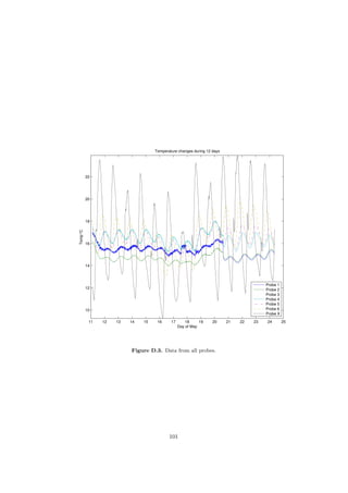
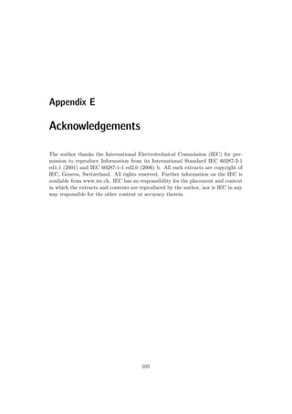
As can be seen in all measurement data (Appendix D figure D.1, D.2, and D.3) the
temperature is not only affected by the heat cable, but also by external sources. The
sinusoidal changes in temperature can be traced to solar radiation. Nothing else in
the area of the duct emits heat and the heat cable has a fixed power. Sensors placed
closer to the surface of the road experiences greater temperature changes with solar
radiation and air temperatures than sensors deeper down in the road [17]. A deeper
placement also means less drying-out of the soil/sand due to external heat (solar
radiation). An increased distance to ground level also decimates the cooling effect
of heat being transferred by air.
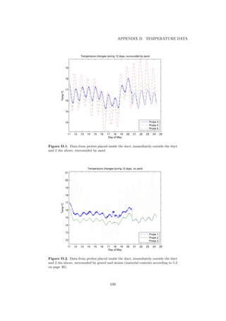
11.2 Surrounding media
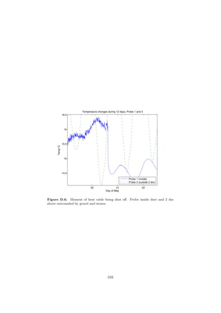
Even though two different kinds of filling were used around the duct and power
cable no significant difference can be found between them. In one case sand was
used and in the other gravel and stones1.
In both cases measurements indicates low thermal resistance. Temperatures inside
and outside the duct changes simultaneously. Compare Probe 4 and 5 in figure D.1
in appendix D to see the almost unnoticeable differences.
1
See section 5.3 for details.
59](https://image.slidesharecdn.com/ampacityaccordingtoiec-60287-191019201759/85/Ampacity-according-to-iec-60287-71-320.jpg)
![CHAPTER 11. ANALYSIS OF EXPERIMENTAL DATA
11.3 Temperature
A power cable placed directly in soil without protective duct emits heat immediately
into surrounding media. The ability of the system to transfer heat depends entirely
on the thermal properties of the soil/sand. Introducing a plastic duct to the system
means additional thermal resistance. Heat produced due to losses in the power
cable is not transferred as easily as in the case where no protective layers surround
the power cable.
11.4 Duct
The soil/gravel surrounding the plastic duct has a thermal resistivity of approxi-
mately 1 Km/W [6]. The duct itself has a thermal resistivity of around 6 Km/W.
A material with high thermal resistivity has a low ability of heat transfer2. The
impact from the duct’s thermal resistance can be seen in figure D.1 in appendix D
and table 11.1 where indications are found supporting the theory that the duct both
aggravates heat transfer and prevents further heating. In figure D.1 the difference
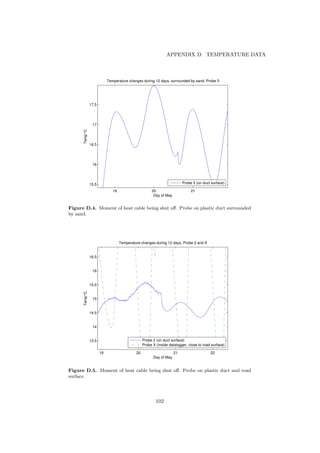
in temperature between the sensors placed inside the duct and immediately outside
can be seen. The thermal resistance of the duct cause a ≈0.4°C higher temperature
inside the duct than outside (when external heat sources affect the system less than
internal sources). When external heat sources affects the duct and power cable more
than the heat cable, the duct works in the opposite way and protects the inside from
heating up (in this case ≈0.5°C difference). After digging up both plastic ducts no
damages were found on model SRN110 (see section 5.3). Small punctures where
found on duct model SRS110 due to the coarse structure of the surrounding gravel.
11.5 Temperature restriction
One of the most important parts of the results from the experiment can be seen
in figure 11.1 on page 62 where the continuous line marks temperatures inside the
duct surrounded by sand.
To understand how heat was conducted throughout the system the heat cable was
turned off and the temperature sensors left to observe the result. Between the 20th
and the 21st of May a sharp change in temperatures can be seen due to this heat
restriction. From this one figure it is only possible to get a vague idea of what
kind of change has occurred. However, comparing the result in figure 11.1 with the
mean temperatures of the surroundings in table 11.1 on page 61 can give additional
information regarding the thermal resistivity of the system.
2
As stated by Fourier’s law, the thermal analogue of Ohm’s law.
60](https://image.slidesharecdn.com/ampacityaccordingtoiec-60287-191019201759/85/Ampacity-according-to-iec-60287-72-320.jpg)
![11.6. CIRCUMSTANCES
When transients for system heat up/cool down (see figure 11.2) has been accounted
for3, mean temperature values were calculated. The mean values in table 11.1 are
used to confirm changes in temperature throughout the system. During the time
the heat cable is on it emits heat and affects the system surrounding it (see section
5.3 details on set-up).
Probes 1,2 and 3 are placed in the vicinity of the gravel covered duct while probes 4,
5 and 6 are placed close to the sand covered duct. Table 11.1 on page 61 describes
mean temperatures based on data gathered by probes 1-6 according to figure 5.3
on page 32. ¯θon is the temperature when the heat cable is turned on. ¯θoff is the
temperature when the heat cable is turned off. ∆¯θ is the difference in temperature
between on and off . Negative difference means that the mean temperature was
higher with the heat cable turned off than on. This is an effect of the heat from the
sun.
Table 11.1. Mean temperatures with heat cable on and off.
Mean temperatures
Sensor n ¯θn,on [°C] ¯θn,off [°C] ∆¯θn
1 15.5 14.8 0.7
2 14.5 14.9 -0.4
3 15.6 17.2 -1.6
4 16.4 16.3 0.1
5 16.0 16.7 -0.7
6 15.9 17.6 -1.7
11.6 Circumstances
When the experiment equipment (see section 5.2 on page 29) was installed it was
done with regards to how the road is normally built. This means that no special
regard was shown to sensors and data loggers installed in the road. To prepare the
road for heavy traffic, the road surface is flattened with a heavy duty soil compactor.
This means two things:
1. The circumstances for the experiment (properties of the road material, geom-
etry of the cable versus road surface, etc.) were similar to how they would be
during a full scale application.
2. The equipment might have been affected by vibrations or other forces from
the road preparation machines.
3
Extreme values in the beginning of data gathering (when sensors are still not buried) are
neglected, see figure 11.2.
61](https://image.slidesharecdn.com/ampacityaccordingtoiec-60287-191019201759/85/Ampacity-according-to-iec-60287-73-320.jpg)
![11.7. SUMMARY OF EXPERIMENTAL DATA ANALYSIS
0 10 20 30 40 50 60 70 80 90
20
22
24
26
28
30
32
34
36
Temp°C
Time *5*60 [s]
Figure 11.2. Heat up/cool down transient for system surrounded by sand. The
peak represents the installation process when the sensor is placed above ground level
(in the sun).
63](https://image.slidesharecdn.com/ampacityaccordingtoiec-60287-191019201759/85/Ampacity-according-to-iec-60287-75-320.jpg)

![Chapter 12
Analysis of Time, Cost & Logistics Data
In this chapter some of the advantages of each method will be analysed. Time, cost
and logistics are all important to accurately evaluate the value in the two competing
power cable placement methods. The chapter following after Analysis is the chapter
Conclusions & Future which is based on results from the analysis.
12.1 Time
The challenging method for cable placement1 differs from the existing method when
it comes to time extent. In table 9.1 the difference between the two methods can be
seen. The method of placing the power cable in a trench implies the construction of
the trench and the placement of the cable. In the challenging method however, no
trench is constructed, but a duct is placed in the road while constructing it. Vice
versa, the trench method does not include any handling of a plastic duct. According
to contractors (Mikael Karlsson [18], Christer Liljegren [19] and Statkraft employees
Urban Blom [21] and Kjell Gustafsson [20]) the placement of a duct in the road takes
less time than the construction of a trench. The duct method takes 37 hours/km
power cable (where additional road work is included) compared to 83 hours/km
power cable using the conventional method with power cable placed in a trench.
Another benefit of the duct method is that the decreased installation time creates
more flexibility for power cable establishment during different phases of the project.
12.2 Cost
In table 9.2 the actual material needs are presented. The need for cover-sand is high
in the existing method, but on the other hand no duct is used in the trench. 100
m3 sand is an approximation, but the need for sand is extensive2. In the suggested
1
Power cable placed in a plastic duct underneath the road instead of directly in the ground in
a trench next to the road.
2
100 m3
sand cost approximately 200 SEK/m3
65](https://image.slidesharecdn.com/ampacityaccordingtoiec-60287-191019201759/85/Ampacity-according-to-iec-60287-77-320.jpg)
![CHAPTER 12. ANALYSIS OF TIME, COST & LOGISTICS DATA
new method no additional sand is needed3, but this method demands the use of a
plastic duct. To place the power cable inside the plastic duct, special power cable
push and pull equipment is used. This equipment is not needed when placing the
power cable in a trench.
12.3 Logistics
Already mentioned in section 12.2, one of the big differences between the two com-
peting power cable placement methods is that when using a duct the power cable
is pushed in after the duct has been buried. To perform the pushing of the power
cable special power cable pushing equipment is required. According to Mikael Karls-
son [18] pushing the power cable into the duct takes approximately 10 hours per
kilometer power cable (including joining). See table 9.1 and 9.5 for details. In the
trench scenario 150 m3 of excavation will have to be removed. At least 12 trips
with a 13-ton loader is demanded to cover the demand for sand4 in the trench. Ap-
proximately 220 tons of excavation material is removed in the conventional method.
That would require some 17 truck loads to remove. The soil removed when digging
the trench can not be used again due to it’s coarse structure (risk of power cable
damages).
12.4 Summary of time, cost & logistics data analysis
In both time, cost and logistics the two chosen methods differ. Where a duct
is used, time is saved when no trench is needed. Higher flexibility is obtained
when power cable installation can be performed during greater part of the project.
Project costs are decimated when no additional excavation or material is needed
for cable installation. Logistics advantages affect both time and cost. The amount
of additional transports for sand and excavation material are considerably reduced.
Only the sand needed for trench construction weighs approximately 145 tons and
it would take one truck 5 12 trips to move that amount. In the duct method no
machines used for cable trench construction will use the finished road.
3
The sand in the road is used to cover the duct
4
100 m3
sand weighs approximately 145 tons.
5
13 tons loading capacity.
66](https://image.slidesharecdn.com/ampacityaccordingtoiec-60287-191019201759/85/Ampacity-according-to-iec-60287-78-320.jpg)


![Chapter 14
Conclusions
All power cables are limited in terms of ability to withstand high temperatures.
High operating temperatures affects the sheath and most other components of the
cable. Component functionality may be compromised with an increase in thermal
stress. Hence, the lifetime of the cable is dependent on that the maximum contin-
uous operating temperature never exceeds that of the manufacturers specification.
Exceeding the specifications of the manufacturer can lead to hardening of flexible
plastics, punctuating of protective layers, deterioration of cable armour, dry out
of surrounding soil, etc. All these degradations can lead to the power cable being
less resilient to outer forces (e. g. sharp rocks), troubled by short circuits, struck
by water leakage, affected by decreasing ampacity and increasing thermal resistance.
If the power cable, on the other hand, is well adapted (rated) to reigning circum-
stances (dry soil, shifting load, etc.) it is according to section 3.1 less likely to
deteriorate and demanded ampacity levels can be maintained.
When using the conventional method for placing power cables in wind power farms
the issue of road usage is another of the big challenges. Can the time be divided
between different contractors to reach the ultimate solution? As stated in the guide-
lines [12] for this project, the suggested method for power cable placement aims to
decrease unfavourable interaction (simultaneous use of the road) between contrac-
tors. As presented in chapter 13 on page 67 the method using plastic ducts buried
in the road creates a far more flexible environment for additional contractors using
the road.
Since the above conclusion easily can be controlled, it might seem strange that the
new method has not been tried earlier. In this case, the ampacity of the power
cable placed in the plastic duct is a very important property that is not as easy to
measure as the difference in time between two cable placement methods.
One change that could have given better results during thermal resistance measure-
ments was the dimensioning of the heat cable installed in the duct. Even though
71](https://image.slidesharecdn.com/ampacityaccordingtoiec-60287-191019201759/85/Ampacity-according-to-iec-60287-83-320.jpg)
![14.3. WIND POWER FARM
sand transports are needed (see section 12.3). All transports of additional3 sand
and excavation material is eliminated in the duct method. Costs decrease when
no additional material is needed to construct trenches and no additional excavation
transports are needed since the duct is placed within the road. The heavy duty
quality of the duct makes it possible to reuse the coarse excavated material from
road construction. According to table 9.4 the conventional method cost ≈108000
SEK/km finished road and placed power cable4. The duct method is approximated
to cost 88000 SEK/km finished road and placed power cable. Logistics Usage of
the road is more flexible than with the conventional method since the roads are not
used for neither trench construction nor power cable placement. This logistic ad-
vantage leads to time savings and in the end decreased cost. Placing the duct in the
road adds approximately 27 hours of additional delay per kilometer, but minimizes
the simultaneous use of the finished road. Placing the cable the conventional way
demands approximately 70 hours of simultaneous road usage per kilometer.
14.3 Wind power farm
With regards to analysis and conclusions this section will contain calculations ap-
proximating the impact on projects involving several wind power plants. In this
case a 10 power plant farm is treated.
A farm with 10 power plants demand an area of approximately 1150x1230 m2 (based
on Wind farm configuration on page 236 in Wind Power Projects (2008), T Wizelius
[10]). Assuming the wind farm is located close to the public grid (≈3 km) it is
possible to calculate the need for logistics as well as time demand and cost. Given
that the farm is constructed in an optimal way a total of ≈8 km power cable5 is
demanded. Table 14.1 shows the total cost of a 10 wind power plants farm (regarding
power cable placement). The power cable placement methods differ in time demand
and based on the 10 power plant suggestion the conventional method would require
(83-37) h*8 km=368 man-hours more than the duct-method.
14.4 Summary
Based of results gathered according to chapter 4, 5 and 6, analysed in chapter 10
the method where the power cable is placed underneath the road in a plastic duct
is considered advantageous compared to conventional methods. Using a duct offers
improved solutions in areas such as logistics, cost and time demand.
3
Sand and excavation material is still transported in both methods when the road is constructed.
4
The cost is defined as "cost above mutual cost" where the construction of the road is a common
cost for both methods.
5
1 km connecting power plants three and three, 1 km to join all plants and 3 km to extend the
power cable towards connection on public grid.
73](https://image.slidesharecdn.com/ampacityaccordingtoiec-60287-191019201759/85/Ampacity-according-to-iec-60287-85-320.jpg)
![CHAPTER 14. CONCLUSIONS
Table 14.1. Approximations regarding a wind power farm with 10 power plants.
Cost [SEK]
Item Conventional Duct
Sand 162400 0
Plastic duct 0 400000
Cable pusher 0 48000
Man-hours 510000 222000
Transport 188640 (ex fuel) 0
Total 861040 670000
The protection from the plastic duct allows the power cable to be placed in an
apparent exposed position. Rocks and other coarse road fillings does not affect the
plastic duct or power cable in an observable way. Cables placed in a trench next
to the road (without duct) are highly dependant on a surrounding of sand and the
absence of rocks and stones. The depth of the placement is crucial for power cable
capacity (ampacity) in both the conventional method and the method using a plas-
tic duct. Ambient temperature of the air above ground and solar radiation affects
the temperature of the power cable can be avoided by deeper placement. The sur-
rounding material also affects the ampacity and can be selected to compensate for
disadvantages created by shallow placement. Materials with low thermal resistance
should be chosen.
When implementing the method using plastic ducts there are advantages regarding
both costs and construction time. A faster construction time is not obvious to be a
certain gain. If cost increases and logistics grow more complex a quick construction
time does not always lead to sought benefits. But if time savings is combined with
enhancements in at least one of the areas cost or logistics advantages could be found.
Complex logistic planning is one of the issues that can be avoided (or at least
simplified) with this new method for power cable placement. The fact that one
contractor less will use the road after it’s finishing solves many unnecessary conflicts
and/or contractor "clashes". Plans of road usage are simplified with the new method.
74](https://image.slidesharecdn.com/ampacityaccordingtoiec-60287-191019201759/85/Ampacity-according-to-iec-60287-86-320.jpg)


![Bibliography
16.1 International Standards
[1] IEC 60287-1-1 ed2.0; Electric cables - Calculation of the current rating - Part
1-1: Current rating equations (100 % load factor) and calcuation of losses -
General. Copyright ©International Electrotechnical Commission (IEC) Geneva,
Switzerland, www.iec.ch, 2006
[2] IEC 60287-2-1 ed1.1; Electric cables - Calculation of the current rating -
Part 2-1: Thermal resistance - Calculation of the thermal resistance. Copy-
right ©International Electrotechnical Commission (IEC) Geneva, Switzerland,
www.iec.ch, 2001
[3] IEC 60287-3-2; Electric cables - Calculation of the current rating - Part 3-2:
Sections on operating conditions - Economic optimization of power cable size.
International Electrotechnical Commission, 1995-06
16.2 Books & Publications
[4] George J Anders; Rating of Electric Power Cables in Unfavorable Thermal
Environment. IEEE Press, 445 Hoes Lane, Piscataway, NJ 08854, ISBN 0-471-
67909-7, 2005.
[5] George J Anders; Rating of electric power cables: Ampacity computations for
transmission, distribution and industrial applications. IEEE Press, 345 East
47th Street, New York, NY, IEEE ISBN 07803-1177-9, 1997.
[6] ABB; XLPE Cable Systems - User’s guide. ABB power Technologies AB, Karl-
skrona, Sweden, 5th edition, 2010.
[7] Irving M Gottlieb; Practical Transformer handbook. Linacre House Jordan Hill,
Oxford OX28DP, ISBN 0 7506 3992 X, 1998.
[8] R K Rajput; Power System Engineering. Laxmi Publications LTD, Golden
House, Daryaganj, New Delhi-110002, First edition, 2006.
79](https://image.slidesharecdn.com/ampacityaccordingtoiec-60287-191019201759/85/Ampacity-according-to-iec-60287-91-320.jpg)
![BIBLIOGRAPHY
[9] IUPAC; IUPAC Compendium of Chemical Terminology - The Gold Book. Royal
Society of Chemistry, Cambridge, UK, 2nd Edition, (1997).
[10] Tore Wizelius; Developing wind power projects - theory & practice. Studentlit-
teratur, ISBN 978-1-84407-262-0, third edition, 2007.
[11] Hans Edin, Dimensionering av kabelanläggningar för distributionsnät.. Kung-
liga Tekniska Högskolan, Stockholm, 2009-11-26.
[12] Kjell Gustafsson, Projektförslag. Statkraft Sverige AB, Stockholm, 2011.
[13] Leslie Lamport; LATEX: A Document Preparation System. Addison Wesley,
Massachusetts, 2nd Edition, 1994.
16.3 Internet
[14] Electropedia; The World’s Online Electrotechnical Vocabulary.
http://www.electropedia.org, accessed March 15th, 2011.
[15] The Swedish Transport Administration; Guidelines for construction of roads.
http://publikationswebbutik.vv.se/upload/4167/2008_78_vvtk_vag.pdf, ac-
cessed May 15th, 2011.
[16] Elektroskandia;
Electrotechnic wholesale dealer. http://www.elektroskandia.se, accessed June
1st, 2011.
[17] Lyndon State College; Atmospheric Sciences.
http://apollo.lsc.vsc.edu/classes/met455/notes/section6/2.html, accessed June
11th, 2011.
16.4 Meetings & Interviews
[18] Mikael Karlsson, Mikael Karlssons Gräv & Röj. 2011.
[19] Christer Liljegren, Eltel Networks. 2011.
[20] Kjell Gustafsson, Responsible electric grid, Statkraft Sverige AB, Vind. 2011.
[21] Urban Blom, Statkraft Sverige AB, Vind. 2011.
80](https://image.slidesharecdn.com/ampacityaccordingtoiec-60287-191019201759/85/Ampacity-according-to-iec-60287-92-320.jpg)
![Appendix A
Detailed Description of IEC-60287
The following appendix is in it’s entirety a summary of the exact wording of IEC-
60287. See chapter E for acknowledgement. In IEC-60287-1-1 [1] the ampacity of
an AC cable is derived from the expression for the temperature rise of the cable
conductor above ambient temperature:
∆θ = (I2
R +
1
2
Wd)T1 + [I2
R(1 + λ1) + Wd]nT2 + [I2
R(1 + λ1 + λ2) + Wd]n(T3 + T4)
(A.1)
where
I is the current flowing in one conductor [A];
∆θ is the conductor temperature rise above the ambient temperature [K];
NOTE The ambient temperature is the temperature of the surrounding medium under normal
conditions, at a situation in which cables are installed, or are to be installed, including the effect
of any local source of heat, but not the increase of temperature in the immediate neighbourhood
of the cables due to heat arising therefrom.
R is the alternating current resistance per unit length of the conductor at
maximum operating temperature [Ω/m];
Wd is the dielectric loss per unit length for the insulation surrounding the con-
ductor [W/m];
T1 is the thermal resistance per unit length between one conductor and the
sheath [Km/W];
T2 is the thermal resistance per unit length of the bedding between sheath and
armour [Km/W];
T3 is the thermal resistance per unit length of the external serving of the cable
[Km/W];
81](https://image.slidesharecdn.com/ampacityaccordingtoiec-60287-191019201759/85/Ampacity-according-to-iec-60287-93-320.jpg)
![APPENDIX A. DETAILED DESCRIPTION OF IEC-60287
T4 is the thermal resistance per unit length between the cable surface and the
surrounding medium [Km/W];
n is the number of load-carrying conductors in the cable (conductors of equal
size and carrying the same load);
λ1 is the ratio of losses in the metal sheath to total losses in all conductors in
that cable;
λ2 is the ratio of losses in the armouring to total losses in all conductors in
that cable.
A.0.1 Buried cables where drying-out of the soil does not occur
The permissible current rating is obtained from 4.1 according to IEC 60287-1-1 [1]
as follows:
I =
∆θ − Wd[0.5T1 + n(T2 + T3 + T4)]
R[T1 + n(1 + λ1)T2 + n(1 + λ1 + λ2)(T3 + T4)]
0.5
[A] (A.2)
A.0.2 Buried cables where partial drying-out of the soil occurs
The permissible current rating is obtained from 4.1 according to IEC 60287-1-1 [1]
as follows:
I =
∆θ − Wd[0.5T1 + n(T2 + T3 + vT4)] + (v − 1)∆θx
R[T1 + n(1 + λ1)T2 + n(1 + λ1 + λ2)(T3 + vT4)]
0.5
[A] (A.3)
where
v is the ratio of the thermal resistivities of the dry and moist soil zones
(v = ρd/ρw);
ρd is the thermal resistivity of the dry soil [Km/W];
ρw is the thermal resistivity of the moist soil [Km/W];
θx is the critical temperature rise of the soil and temperature of the boundary
between dry and moist zones [°C];
θa is the ambient temperature [°C];
∆θx is the critical temperature rise of the soil. This is the temperature rise of the
boundary between the dry and moist zones above the ambient temperature
of the soil (θx − θa) [K];
82](https://image.slidesharecdn.com/ampacityaccordingtoiec-60287-191019201759/85/Ampacity-according-to-iec-60287-94-320.jpg)
![A.1. CALCULATION OF LOSSES
θx and ρd shall be determined from a knowledge of the soil conditions.
NOTE The soil parameters may be agreed between power cable manufacturer and purchaser.
A.1 Calculation of losses
A.1.1 AC resistance of conductor
The a.c. resistance per unit length of the conductor at its maximum operating
temperature is given by the following formula:
R = R (1 + ys + yp) [Ω] (A.4)
where
R is the current resistance of conductor at maximum operating temperature
[Ω/m];
R is the d.c. resistance of conductor at maximum operating temperature [Ω/m];
ys is the skin effect factor;
yp is the proximity effect factor.
DC resistance of conductor
R = R0[1 + α20(θ − 20)] [Ω] (A.5)
where
R0 is the d.c. resistance of the conductor at 20 °C [Ω/m];
NOTE R0 is calculated using the equation for resistance of a conductor of
uniform cross section: R0 = ρL
A
where
ρ is the resistivity of aluminium at 20 °C [Ω · m];
L is the length of the conductor in [m];
A is the cross section area of the conductor in [m2].
α20 is the constant mass temperature coefficient for aluminium at 20 °C per
Kelvin;
θ is the maximum operating temperature in °C.
83](https://image.slidesharecdn.com/ampacityaccordingtoiec-60287-191019201759/85/Ampacity-according-to-iec-60287-95-320.jpg)
![APPENDIX A. DETAILED DESCRIPTION OF IEC-60287
Skin effect factor ys
The skin effect factor ys is given by:
ys =
x4
s
192 + 0.8 · x4
s
(A.6)
where
x2
s =
8πf
R
· 10−7
· ks (A.7)
f is the supply frequency in hertz.
Proximity effect factor yp (for three-core cables)
The proximity effect factor is given by:
yp =
x4
p
192 + 0.8x4
p
dc
s
2
0.312 ·
dc
s
2
+
1.18
x4
p
192+0.8x4
p
+ 0.27
(A.8)
where
x2
p =
8πf
R
· 10−7
· kp (A.9)
dc is the diameter of conductor [mm];
s is the distance between conductor axes [mm].
A.1.2 Dielectric losses
The dielectric loss per unit length in each phase is given by:
Wd = ωCU2
0 tan δ [W/m] (A.10)
where
ω = 2πf;
C is the capacitance per unit length [F/m];
U0 is the voltage to earth [V ].
84](https://image.slidesharecdn.com/ampacityaccordingtoiec-60287-191019201759/85/Ampacity-according-to-iec-60287-96-320.jpg)
![A.1. CALCULATION OF LOSSES
The capacitance for circular conductors is given by:
C =
ε
18 ln Di
dc
· 10−9
[F/m] (A.11)
where
ε is the relative permittivity of the insulation;
Di is the external diameter of the insulation (excluding screen) [mm];
dc is the diameter of conductor, including screen, if any [mm].
A.1.3 Loss factor for sheath and screen
The power loss in the sheath or screen ( λ1 ) consists of losses caused by circulating
currents ( λ1 ) and eddy currents ( λ1 ), thus:
λ1 = λ1 + λ1 (A.12)
The formulae given in this section express the loss in terms of the total power loss
in the conductor(s).
RS = RS0 [1 + α20(θSC − 20)] [Ω/m] (A.13)
where
RS0 is the resistance of the cable sheath or screen at 20 °C [Ω/m].
λ1 =
RS
R
1
1 + RS
X
2 (A.14)
where
RS is the resistance of sheath or screen per unit length of cable at its maximum
operating temperature [Ω/m];
X is the reactance per unit length of sheath or screen per unit length of cable
= 2ω · 10−7 ln 2s
d [Ω/m];
ω = 2πf [1/s];
s is the distance between conductor axes in the electrical section being con-
sidered [mm];
d is the mean diameter of the sheath [mm];
85](https://image.slidesharecdn.com/ampacityaccordingtoiec-60287-191019201759/85/Ampacity-according-to-iec-60287-97-320.jpg)
![APPENDIX A. DETAILED DESCRIPTION OF IEC-60287
λ1 = 0. The eddy-current loss is ignored according to IEC 60287-1-1 section
2.3.1 [1].
The eddy-current loss λ1 is ignored according to IEC 60287-1-1 section 2.3.1 [1].
A.2 Thermal resistance
A.2.1 Thermal resistance of constituent parts of a cable
Thermal resistance between one conductor and sheath T1
For screened cables with circular conductors the thermal resistance T1 is:
T1 =
ρT
2π
G (A.15)
where
G is the geometric factor according to IEC60287 [2];
ρT is the thermal resistivity of insulation [Km/W];
Thermal resistance between sheath and armour T2
AXKJ-F 3x95/25 does not contain armour nor metallic sheath. Hence T2 is not
considered.
Thermal resistance of outer covering (serving) T3
T3 =
ρT
2π
· ln 1 +
2t3
Da
(A.16)
where
t3 is the thickness of serving [mm];
Da is the external diameter of the armour [mm];
A.2.2 External thermal resistance T4
The external thermal resistance of a cable in a duct consists of three parts:
T4 is the thermal resistance of the air space between the cable surface and
duct’s internal surface;
T4 is the thermal resistance of the duct itself;
T4 is the external thermal resistance of the duct.
T4 = T4 + T4 + T4 (A.17)
86](https://image.slidesharecdn.com/ampacityaccordingtoiec-60287-191019201759/85/Ampacity-according-to-iec-60287-98-320.jpg)
![A.2. THERMAL RESISTANCE
Thermal resistance between cable and duct T4
T4 =
U
1 + 0.1(V + Y θm)De
(A.18)
where
De is the external diameter of the cable [mm];
θm is the mean temperature of the medium filling the space between cable and
duct. An assumed value has to be used initially and the calculation repeated
with a modified value if necessary [°C];
Thermal resistance of the duct T4
T4 =
ρT
2π
· ln 1 +
D0
Dd
(A.19)
where
D0 is the outside diameter of the duct [mm];
Dd is the inside diameter of the duct [mm];
ρT is the thermal resistivity of duct material [Km/W]
External thermal resistance of the duct T4
T4 =
1
2π
ρT · ln (2u) (A.20)
where
ρT is the thermal resistivity of the soil [Km/W];
u = 2L
D0
, L is the placement depth [mm];
87](https://image.slidesharecdn.com/ampacityaccordingtoiec-60287-191019201759/85/Ampacity-according-to-iec-60287-99-320.jpg)

![APPENDIX B. DETAILED DESCRIPTION OF CALCULATIONS ACCORDING TO
IEC-60287
DC resistance of conductor
R = R0[1 + α20(θ − 20)] (B.2)
where R0 is the dc resistance of the conductor at 20 °C.
R0 = ρL
A = ρ = ρaluminium = 2.8264 · 10−8 [Ω · m], L = 1 [m], A = 95 · 10−6 [m2] =
= 2.8264 · 10−8 1
95·10−6 = 0.00029752 [Ω/m]
and α20 = 4.03 · 10−3 [ 1
K ], θ = 90 °C
→ R = R0[1 + α20(θ − 20)] = 0.00029752 · [1 + 4.03 · 10−3(90 − 20)]Ω =
0.00038144 Ω
Skin effect factor ys
ys =
x4
s
192 + 0.8 · x4
s
(B.3)
where
xs =
8πf
R
· 10−7 · ks = {ks = 1} =
8π50
0.00038144
· 10−7 = 0.57397
→ ys =
0.573974
192 + 0.8 · 0.573974
= 0.00056501
Proximity effect factor yp (for three-core cables)
The proximity effect factor is given by:
yp =
x4
p
192 + 0.8x4
p
dc
s
2
0.312 ·
dc
s
2
+
1.18
x4
p
192+0.8x4
p
+ 0.27
(B.4)
where
xp =
8πf
R
· 10−7 · kp = {kp = 0.8} =
8π50
0.00038144
0.8 · 10−7 = 0.26355
dc=12 mm, the diameter of the conductor;
s=30 mm, the distance between conductor axes.
90](https://image.slidesharecdn.com/ampacityaccordingtoiec-60287-191019201759/85/Ampacity-according-to-iec-60287-102-320.jpg)
![B.2. CALCULATION OF LOSSES
→ yp =
0.263554
192 + 0.8 · 0.263554
12
30
2
0.312 ·
12
30
2
+
1.18
0.263554
192+0.8·0.263554 + 0.27
= 0.00025545
→ R = R (1 + ys + yp) = 0.00038144 · (1 + 0.00056501 + 0.00025545) Ω =
0.0038175 Ω
B.2.2 Dielectric losses
The dielectric loss per unit length in each phase is given by:
Wd = ωCU2
0 tan δ (B.5)
ω = 2πf = {f = 50 Hz} = 2π50 rad/s;
U0 = 36√
3
· 103 = V, the voltage to earth;
tan δ=0.004, loss factor of the insulation (XLPE).
The capacitance for circular conductors is given by:
C =
ε
18 ln Di
dc
· 10−9
=
2.5
18 ln 28
12
· 10−9
F/m = 0.16392 · 10−9
F/m (B.6)
ε=2.5, the relative permittivity of the insulation (XLPE);
Di=28 mm, the external diameter of the insulation (excluding screen).
→ Wd = ωCU2
0 tan δ = 2π50·0.16392·10−9
(
36
√
3
·103
)2
·0.004 W/m = 0.088987 W/m
B.2.3 Loss factor (λ1) for screen
λ1 = λ1 + λ1 (B.7)
λ1 =
RS
R
1
1 + RS
X
2 (B.8)
where
X = 2ω · 10−7
ln
2s
d
= 2 · 2π50 · 10−7
ln
2 · 30
55.168
Ω/m ≈ 5.275 · 10−6
Ω/m
RS = RS0 [1 + α20(θSC − 20)] (B.9)
RS0 = ρCU · lSC
ASC
= 1.7241 · 10−8 1
25·10−6 Ω/m = 0.00068964 Ω/m, the resistance of
the cable screen at 20 °C;
91](https://image.slidesharecdn.com/ampacityaccordingtoiec-60287-191019201759/85/Ampacity-according-to-iec-60287-103-320.jpg)
![APPENDIX B. DETAILED DESCRIPTION OF CALCULATIONS ACCORDING TO
IEC-60287
θSC = θ − 20 = 95 − 20 °C=75 °C, the approximated maximum operating temper-
ature of the screen.
RS = 0.00068964 1 + 4.03 · 10−3
(95 − 20) Ω/m = 0.000856394952 Ω/m
λ1 =
RS
R
1
1 + RS
X
2 =
0.000856394952
0.0038175
1
1 + 0.000856394952
5.275·10−6
2 = 8.798 · 10−5
The eddy-current loss λ1 is ignored according to IEC 60287-1-1 section
2.3.1 [1].
λ1 = λ1 + λ1 = 8.798 · 10−5
+ 0 = 8.798 · 10−5
B.3 Thermal resistance T
See section 4.3 for extended explanation of how the thermal resistance T is consid-
ered.
T = T1 + T2 + T3 + T4
B.3.1 Internal thermal resistances, T1, T2 and T3
Thermal resistance between one conductor and sheath T1
T1 =
ρT,PEX
2π
G (B.10)
G ≈1.63, the geometric factor according to IEC60287 [2];
ρT,PEX=3.5 Km/W, the thermal resistivity of PEX insulation.
T1 =
ρT,PEX
2π
G =
3.5
2π
1.63 Km/W = 0.90798 Km/W (B.11)
Thermal resistance between sheath and armour T2
AXKJ-F 3x95/25 does not contain armour nor metallic sheath. Hence T2 is not
considered.
T2 = 0 (B.12)
92](https://image.slidesharecdn.com/ampacityaccordingtoiec-60287-191019201759/85/Ampacity-according-to-iec-60287-104-320.jpg)
![APPENDIX B. DETAILED DESCRIPTION OF CALCULATIONS ACCORDING TO
IEC-60287
ρsoil=1.0 Km/W, the thermal resistivity of earth around bank;
L = 700 mm, the depth of the laying to centre of duct bank;
D0=110 mm, the external diameter of the duct;
u = 2∗L
D0
= 2∗700
110 = 12.73;
T4 =
1
2π
ρsoil · ln (2u) =
1
2π
1.0 · ln (2 · 12.73) Km/W = 0.6137 Km/W (B.21)
T4 = T4 + T4 + T4 = 0.4129 + 0.0817 + 0.6137 Km/W = 1.1083 Km/W (B.22)
B.4 Summary
Table B.1. Ampacity common physical quantities.
Physical
quantity
No dry-out; Par-
tial dry-out; Avoid
dry-out
∆θ 343.15 K
R 0.0038175 Ω/m
Wd 0.088987 W/m
T1 0.90798 Km/W
T2 0 Km/W
T3 0.098588 Km/W
T4 1.1083 Km/W
n 3
λ1 8.798·10−5
λ2 0
B.4.1 Buried cables where drying-out of the soil does not occur
As declared in chapter 4 the ampacity can be calculated according to:
I =
∆θ − Wd[0.5T1 + n(T2 + T3 + T4)]
R[T1 + n(1 + λ1)T2 + n(1 + λ1 + λ2)(T3 + T4)]
0.5
(B.23)
B.4.2 Buried cables where partial drying-out of the soil occurs
The permissible current rating is obtained from 4.1 according to [1] as follows:
94](https://image.slidesharecdn.com/ampacityaccordingtoiec-60287-191019201759/85/Ampacity-according-to-iec-60287-106-320.jpg)
![B.5. AMPACITY IN TWO CASES
I =
∆θ − Wd[0.5T1 + n(T2 + T3 + vT4)] + (v − 1)∆θx
R[T1 + n(1 + λ1)T2 + n(1 + λ1 + λ2)(T3 + vT4)]
0.5
[A] (B.24)
Table B.2. Physical quantities for partial dry-out.
Physical
quantity
Partial dry-out
ρd 3 Km/W
ρw 1 Km/W
v 3
θx 50 °C
θa 20 °C
∆θx 303.15 K
ρd is the thermal resistivity of the dry soil;
ρw is the thermal resistivity of the moist soil;
v =ρd/ρw, the ratio of the thermal resistivities of the dry and moist soil
zones;
θx is the critical temperature rise of the soil and temperature of the boundary
between dry and moist zones;
θa is the ambient temperature;
∆θx =θx − θa, the critical temperature rise of the soil. This is the temperature
rise of the boundary between the dry and moist zones above the ambient
temperature of the soil.
B.5 Ampacity in two cases
Table B.3. Electric power cable ampacity in two cases.
Specification Ampacity [A]
No dry-out 205
Partial dry-out 180
95](https://image.slidesharecdn.com/ampacityaccordingtoiec-60287-191019201759/85/Ampacity-according-to-iec-60287-107-320.jpg)