Download to read offline


![Abstract
As part of the effort to reduce the cost of offshore wind energy, this thesis addresses the
problem of the design of the infield cable topology for offshore wind farms. The final outcome
of the project is a tool that can be implemented in a more general optimization platform
for offshore wind farm design. Therefore, the main objective is to approximate the optimal
inter-array cable connections in affordable computation times.
A review of the state of the art collection system designs indicates the radial and branched
designs as the designs with the highest potential among the conceptual designs. The key
target of the optimization procedure is the minimization of cable cost. Regarding the de-
sign constraints, cable capacities are respected and inter-array cable crossings are strictly
avoided. The literature review of the related research reveals the complexity of the problem
and pinpoints the use of heuristic methods.
Planar Open Savings (POS) [1] and Esau-Williams (EW) [2] heuristics are chosen to treat the
single cable radial and branched designs respectively. Both algorithms are saving heuristic
methods, starting from a star design. At each iteration, the merging of two routes is considered
that could yield to the maximum cost saving. After the implementation of the algorithms is
validated, a methodology is proposed to allow the possibility for multiple cable types.
The behaviour of the heuristics is evaluated both cost and time-wise in a wide range of
instances. The results show that the parameters that differentiate their behaviour are the
use of single or multiple cable types and the position of the substation, which can be located
either centrally or outside the area of the farm. Moreover, a hybrid approach between POS
and EW is developed that improves the performance of EW for multiple cable types. Finally,
specific recommendations are made regarding the use of the best algorithm for each case.
The practicality of the developed tool is enhanced by including the possibility to choose
the switchgear configuration and by eliminating the crossings between inter-array cables and
transmission lines. Last, modifications allow the minimization of crossings with pipelines/ca-
bles that are possibly laid on the seabed. Throughout the report, the comparison of results
provided by the tool with the actually installed layouts shows the prospects of inter-array
cable cost reductions.
Master of Science Thesis Georgios Katsouris](https://image.slidesharecdn.com/cb0cac47-df4b-46e2-bb4a-18b83a544a68-160810174410/85/Georgios_Katsouris_MSc-Thesis-7-320.jpg)


![Chapter 1
Introduction
This Chapter presents the motivation for this Master Thesis. First, the importance of op-
timization in offshore wind farms is outlined with emphasis given to the inter-array cable
topology. Next, the problem statement and the objectives are described and finally, the
layout of the report is given.
1-1 Motivation
The continuously increasing energy demand which has led to the depletion of fossil fuels
alongside with the evident signs of climate change have escalated the efforts towards an
energy transition. Over the past years, Renewable Energy Sources (RES) such as solar,
biomass, geothermal, hydroelectric and wind energy have emerged as potential alternatives
to fossil fuels. The main driver behind this transition is the fact that the exploitation of RES
can reduce the global warming emissions and offer secure and inexhaustible energy supply.
The regulations which have been established in an international level, among which the most
significant are the Kyoto Protocol and European Commission 20-20-20 targets, contributed to
the implementation of RES. The penetration of RES reached 19% of the global final energy
consumption for 2011 where particularly, Wind Energy was 39% of the global renewable power
added in 2012 [3].
Furthermore, over the past decade Offshore Wind Farms (OWF) have gained attention as
power stations. The increased wind potential and the area availability compared to onshore
sites are the key factors for the offshore wind energy exploration. The European Wind Energy
Association (EWEA) predicts installed capacity in Europe to rise from currently 8 GW to
150 GW by 2030, meeting 14% of EU electricity demand [4].
However, a highly dissuasive factor for the further implementation of offshore wind energy
still is the relatively high Levelized Cost of Electricity (LCOE) compared to fossil fuels and
other RES, mainly due to high investment and operation and maintenance costs. Particu-
larly, compared to an onshore wind farm where costs are dominated by the wind turbine,
Master of Science Thesis Georgios Katsouris](https://image.slidesharecdn.com/cb0cac47-df4b-46e2-bb4a-18b83a544a68-160810174410/85/Georgios_Katsouris_MSc-Thesis-19-320.jpg)
![2 Introduction
as far as OWF are concerned the wind turbines, support structures, electrical infrastructure,
installation and maintenance all contribute significantly to the LCOE. Figure 1-1 presents
the capital cost breakdown of an OWF.
Figure 1-1: Capital cost breakdown for typical OWF [5].
In an effort to reduce the LCOE of offshore wind energy, research has been focused on the
optimization of the design of OWF, a multidisciplinary procedure which is required to take
into account the interactions between various parts of the system. One of the most important
design decisions includes the spacing between wind turbines, which directly affects the wake
losses and the cost of the inter-array cables. The latter, as it can be seen in Figure 1-1,
account for 7% of the capital cost. By taking into account the cable losses and the issue
of reliability, the optimization of the inter-array cable topology becomes vital for the design
procedure.
The review of the literature (Section 3-2) indicates that the optimization of the electric design
of OWF has developed relatively recently. Moreover, emphasis has been placed on finding
the optimal solution for the transmission of the generated power from the substation to the
onshore connection point. Considering also the plans for the North Sea Offshore Grid [6], the
optimization problem of the electric layout is narrowed down to the area of the farm. Thus,
the current project is intended to contribute to the infield cable optimization of OWF.
1-2 Objective
Taking into account all the above, the objective of the project can be summarised as follows:
Given the position of the turbines and substations, find the optimal inter-array cable topology
Georgios Katsouris Master of Science Thesis](https://image.slidesharecdn.com/cb0cac47-df4b-46e2-bb4a-18b83a544a68-160810174410/85/Georgios_Katsouris_MSc-Thesis-20-320.jpg)

![Chapter 2
Electrical Collection System for
Offshore Wind Farms (OWF)
This Chapter gives an overview of the electrical system of OWF and then focuses on the
collection system by presenting its conceptual designs and the design requirements.
2-1 Electrical System Overview
The electrical system for OWF usually consists of a medium-voltage electrical collection grid
within the wind farm and a high-voltage electrical transmission system to deliver the power
to an onshore transmission line. Figure 2-1 presents a typical electrical layout of an offshore
wind farm.
Figure 2-1: Typical electrical layout of an offshore wind farm [7].
Master of Science Thesis Georgios Katsouris](https://image.slidesharecdn.com/cb0cac47-df4b-46e2-bb4a-18b83a544a68-160810174410/85/Georgios_Katsouris_MSc-Thesis-23-320.jpg)
![6 Electrical Collection System for OWF
2-1-1 Collection System
The turbine generator voltage is typically 690 V. In order to minimize the losses in the
inter-array cables of the collection system, transformers at each wind turbine step up the
generation voltage to a medium voltage in the range 10 to 35 kV. Also, medium voltage
submarine cables, buried 1 to 2 meters deep in the seabed, are used to inter-connect the wind
turbines and transmit the power to an offshore substation. Section 2-2 presents the typical
configurations that are used for the collection system.
2-1-2 Transmission System
The transmission system starts at the offshore substation, which steps up the voltage to a
transmission voltage of 150 kV. Currently, this is the most common voltage level for submarine
power cables, but it can reach nowadays 500 kV. The high-voltage submarine cables trans-
mit the power to the point of connection with the onshore grid, where possibly an onshore
substation steps up the voltage to match the voltage of the transmission onshore grid.
The two technologies that are used for the transmission system are: High Voltage Alternating
Current (HVAC) and High Voltage Direct Current (HVDC). The key parameter for the choice
between these two technologies is the transmission distance. For distances shorter than 100
km, HVAC is the most economical option whereas for longer distances, HVDC is preferred [8].
Some limiting factors of HVAC include the thermal limitation of cable current and therefore
the limitation of the transmitted power, the significant Ohmic losses of the cables and the
necessary reactive power compensation. On the other hand, HVDC does not need reactive
power compensation, suffers lower electrical losses but has high initial costs because of the
AC/DC and DC/AC converters and filters at both ends of the transmission line.
2-2 Electrical Collection System Designs
There are several configurations for the electrical collection system of OWF. The design
decision depends mainly on the size of the wind farm and the desired level of reliability. In
the past years, the size of OWF was relatively small, thus simplified designs were used for the
collection system and reliability was not taken into account. But as wind farm sizes increase,
the amount of energy lost during a fault might be high enough to overcome the initial costs
of a design that provides reliability to the wind farm. The conceptual designs that are widely
used in OWF, as described in [9], are:
• Radial design, where wind turbines are connected to a single series circuit
• Ring design, where reliability is established through loops between wind turbines
• Star design, where the wind turbines are distributed over several feeders, allowing the
use of lower rated equipment.
Georgios Katsouris Master of Science Thesis](https://image.slidesharecdn.com/cb0cac47-df4b-46e2-bb4a-18b83a544a68-160810174410/85/Georgios_Katsouris_MSc-Thesis-24-320.jpg)
![2-2 Electrical Collection System Designs 7
2-2-1 Radial Design
The most straightforward arrangement of the collection system in a wind farm is a radial
design (Figure 2-2), in which a number of wind turbines are connected to a single cable feeder
within a string. The power rating of the wind turbines and the maximum rating of the cable
within the string determine the maximum number of wind turbines on each string feeder. The
advantages of this design is that it is simple to control, the total cable length is relatively small
and allows the use of low capacity cables further out in each feeder. The major drawback of
this design is its poor reliability as cable or switchgear faults at the end of the radial string
closer to the substation have the potential to prevent all downstream turbines from exporting
power. Nevertheless, it is considered to be the best choice for relatively small OWF.
Figure 2-2: Radial Design [10].
2-2-2 Ring Design
Ringed layouts can supply the reliability, which the radial design lacks of, by incorporating
a redundant path for the power flow within a string. The additional security comes at the
expense of longer cable runs for a given number of wind turbines, and higher cable rating
requirements throughout the string circuit. There are two ring designs for the collection
system, namely the single-sided ring (Figure 2-3) and the double-sided ring (Figure 2-4).
A single-sided ring design requires an additional cable running from the last wind turbine of
the feeder to the substation. This cable must be able to handle the full power flow of the
string in the event of a cable fault connecting the first turbine of the strict to the substation.
The cost of this design is doubled, compared to the cost of a radial layout. However, it is also
the most reliable and the one with the least losses.
Figure 2-3: Single-Sided Ring Design [10].
In a double-sided ring design, the last wind turbine in one string is interconnected to the
last wind turbine in the next string. Compared to the radial design, the cable length will
Master of Science Thesis Georgios Katsouris](https://image.slidesharecdn.com/cb0cac47-df4b-46e2-bb4a-18b83a544a68-160810174410/85/Georgios_Katsouris_MSc-Thesis-25-320.jpg)
![8 Electrical Collection System for OWF
only increase by the distance between the turbines at the end of the feeders. However, the
cables, at least those connecting the first turbines of the feeders to the substation, should
be able to handle the power output of more than double the number of wind turbines which
are connected in a single feeder. This option is thought to be around 60% more expensive
than a radial design but in the long-term and depending on the size of the wind farm and the
possible faults, it can be the most economical choice.
Figure 2-4: Double-Sided Ring Design [10].
Also, the concept of multi-ring design has been proposed. The difference from the double
sided ring is that instead of simply connecting two feeders in parallel, a higher number of
feeders are connected in parallel. The idea is to reduce the high power rating of cables and
equipment which is necessary in the double sided feeder design.
2-2-3 Star Design
The star design, as presented in Figure 2-5, can be used to reduce cable ratings and to
provide a high level of security for the wind farm, since a cable fault can only affect one wind
turbine except for the case when a fault occurs in the feeder cable to the substation. Voltage
regulation along the cables between wind turbines is also likely to be better in this design.
However, cables can be longer and the switchgear more complex, especially at the centre of
the star, so the cost advantage depends on the specific case under study.
Figure 2-5: Star Design [10].
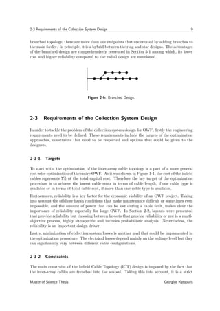
2-2-4 Branched Design
In addition to the aforementioned conceptual designs, the branched design (Figure 2-6), which
is widely used for communication networks, has gained attention for its use in OWF. In a
Georgios Katsouris Master of Science Thesis](https://image.slidesharecdn.com/cb0cac47-df4b-46e2-bb4a-18b83a544a68-160810174410/85/Georgios_Katsouris_MSc-Thesis-26-320.jpg)


![12 The Infield Cable Topology Problem
Merging the set of turbines T and substations S, yields the set of given sites: G = {u1, ..., uG} =
T ∪ S. Now, assuming that the points in G are given in the Euclidean plane, thus discard-
ing any terrain elevation, the distance between two sites uk and uv is equal to: d(uk, uv) =
(uk,1 − uv,1)2
+ (uk,2 − uv,2)2
. Furthermore, including the cost of the cable ri that is in-
stalled between uk and uv, yields the cable cost that is needed to connect these points:
C(uk, uv) = d(uk, uv) ∗ ci. It should be noted that the additional cable cost, induced by the
cable from the bottom of the foundation to the transformer and back down, is irrelevant for
the optimization problem and hence, it is not taken into account.
The solution of the OWFICTP is a set of connections P = {(uk1 , uv1 , rkv
i )1, ..., (ukp , uvp , rkv
i )p}
where uk, uv ∈ G and rkv
i ∈ R and denotes which cable type has been used for the connection
between the nodes uk and uv. This set of connections corresponds to a graph, as it is defined
in graph theory. Thus, the objective function of the optimization problem is the following:
(uk,uv,rkv
i )∈P
d(uk, uv) ∗ ckv
i (3-1)
where d(uk, uv) is the distance between nodes uk and uv and ckv
i is the cost of the cable that
is used for the connection between these nodes.
The cable installation should connect every turbine with exactly one substation over one
distinct path, since ring designs are not treated. Also, the capacity of the cable with the
highest capacity among the available cables ("thickest" cable) should not be exceeded. In
addition, the cables should not cross each other and the option to choose between radial and
branched designs is given to the designer.
3-2 Literature Review
Although research has been focused on the optimization of the transmission system of OWF,
due to its higher cost compared to the collection system, considerable work has been done in
the optimization of the total electrical layout. Moreover, algorithms that have been developed
with a focus on onshore wind farms may be applicable to OWF as well. Hence, this Section
gives an overview of the previous work that has been done in the field.
Dutta [11] optimizes the collector system design of an onshore wind farm with regard to the
cable length. First, she uses a Minimum Spanning Tree (MST) algorithm which is improved
in a second version by allowing Steiner points. In order to incorporate the limitation on
the number of turbines that can be connected on a feeder, she uses k-means clustering for
restricting the maximum number of turbines. Then, the MST is calculated for each cluster.
Last, for each resulting tree, the cable installation can be calculated by selecting a terminal
node and choosing the best cable for transporting the power of the terminal node along its
incident edge.
Berzan et al. [12] decompose the problem in three layers: the Circuit Problem, the Substa-
tion Problem and the Full Farm Problem. The Substation Problem corresponds with the
OWFICTP where only one substation is available. For their model, they consider costs which
take into account the type of cable and the terrain used by the installation. For the single
cable type version of the problem, they formulate it as a Capacitated Minimum Spanning
Georgios Katsouris Master of Science Thesis](https://image.slidesharecdn.com/cb0cac47-df4b-46e2-bb4a-18b83a544a68-160810174410/85/Georgios_Katsouris_MSc-Thesis-30-320.jpg)
![3-2 Literature Review 13
Tree (CMST) Problem and use the Esau-Williams (EW) heuristic to approximate its solu-
tion. They report solutions to problems with up to 1000 turbines but cable crossings are
allowed. Lastly, they do not treat the multiple cable types Substation Problem, where more
than one cable type is available.
Hertz et al. [13] formulate the design of an onshore wind farm collection system as a Mixed-
Integer Linear Programming (MILP) problem. Therefore, they assume that two cable types
are available, one for underground and one for above-ground connections between a set of
nodes which includes the turbines, the substation and transmission line endpoints. After
tightening the MILP formulation by including some cutting planes, they managed to find the
optimal solutions in most instances tested, but they report CPU time of one hour on average.
In his work [14], Fagerfjäll addresses two models: the production model and the infrastructure
model. The cable installation is a subset of the infrastructure model and he also formulates
a MILP version of the problem. The difference with Hertz et al. [13] is that the positions of
the turbines are not fixed. Also, he reports computation times of over 10 minutes to find the
optimal solution for a problem with 30 turbines.
Lumbreras and Ramos [15] have developed an Offshore Wind Farm Layout optimizer (OWL)
that calculates optimal electrical layouts in affordable computation times. Their model re-
ceives the characteristics and positions of wind turbines, the Point of Common Coupling
(PCC) and the possible locations of offshore substations, as well as the cable, transformer
and converter types available and incorporates losses, reliability of the components and wind
scenarios. The problem is formulated as a stochastic Mixed-Integer Programming (MIP).
In order to reduce the computational time, they apply Benders’ Decomposition and Scenario
Aggregation techniques and they use Progressive Contingency Incorporation (PCI) to address
the reliability issue.
One of the first articles that treats explicitly the internal electric connection of Large OWF
was developed by Li et al. [16]. In order to solve the problem, they use a hybrid of genetic and
immune algorithms. After producing the scenarios for the internal connection, they calculate
the annual cost for each alternative, by including power losses in cables and a depreciation
period of the investment of 20 years.
A Genetic Algorithm (GA) has been used also by González-Longatt et al. [17] in order to
find the optimal collection system for large OWF. In their model, they combine the GA with
the classical multiple Traveling Salesman Problem (mTSP) which designs a local collection
system, considering multiple radial feeders connected to the PCC. They report a computation
time of 10.2 minutes for a wind farm with 100 turbines and cable crossings are also allowed.
Bauer and Lysgaard [1] developed a hop-indexed formulation with planarity constraints in
order to find the optimized inter-array cable connections in OWF that are composed only by
open routes, which means that cables cannot cross each other and branching is not allowed.
Also, they adapted the Vehicle Routing Problem (VRP) heuristic of Clarke and Wright to
a Planar Open Vehicle Routing Problem (POVRP) that calculates sub-optimal open routes.
They report on average 2% sub-optimal solutions with a computational time of less than 0.1
s. Also, they treat the optimization problem of two cable types but only for the hop-indexed
formulation.
Master of Science Thesis Georgios Katsouris](https://image.slidesharecdn.com/cb0cac47-df4b-46e2-bb4a-18b83a544a68-160810174410/85/Georgios_Katsouris_MSc-Thesis-31-320.jpg)
![14 The Infield Cable Topology Problem
3-3 Discussion
The OWFICTP is a Non-deterministic Polynomial-time hard (NP-hard) problem in combi-
natorial optimization. In the found literature, different ways to tackle the optimal collection
system of OWF have been developed. Classical mathematical optimization methods with
additional integer constraints and techniques to decompose the problem can produce optimal
solutions in affordable computation times but for relatively medium sized OWF. On the other
hand, hybrids of GA seem promising for optimizing the collection systems of Large OWF.
However, if we take into account the trend for larger OWF in the future, composed by up
to 200 wind turbines, it is not guaranteed that an optimal solution for the collection system
can be found, at least for the time being. On the other hand, sophisticated heuristics have
been developed that can efficiently approximate the optimal solution for the OWFICTP. A
good example, as presented in Section 3-2, that calculated near-optimal open routes, is the
POVRP heuristic developed by Bauer and Lysgaard [1]. Also, EW is considered the most
efficient algorithm for finding a near-optimal solution for the CMST, which corresponds to
the OWFICTP if branched topologies are desirable.
Furthermore, the objective of the thesis is to develop an optimization tool for the collection
system of OWF that can be implemented in a more general optimization platform for OWF
design. Such a platform optimizes every aspect of the design, including the positions of the
wind turbines, support structures, electrical connection scheme and operation and mainte-
nance strategy. In most cases, it is an iterative multidisciplinary procedure that starts from
an initial guess and converges to an optimized design. Thus, it is clear that there is a need
for fast solutions, as close to optimal as possible.
To sum up, heuristics are the only option for providing efficient solutions for NP-hard problems
as the design of the collection system, in terms of computation time and final cost. Therefore,
the focus on the next chapters will be on implementing the most efficient heuristics that have
been developed so far and adapting them to the needs of the OWFICTP.
Georgios Katsouris Master of Science Thesis](https://image.slidesharecdn.com/cb0cac47-df4b-46e2-bb4a-18b83a544a68-160810174410/85/Georgios_Katsouris_MSc-Thesis-32-320.jpg)
![Chapter 4
Radial Offshore Wind Farm Infield
Cable Topology Problem (OWFICTP)
This Chapter treats the radial OWFICTP, where the feeders that connect the turbines to the
substation are in the form of open routes and requirements as cable ratings and the condition
that cables do not cross each other are respected.
4-1 Planar Open Savings (POS) Heuristic
As presented in Section 3-2, POS heuristic, as developed by Bauer and Lysgaard [1], is
one of the most efficient heuristic algorithms for the radial internal connection of Offshore
Wind Farms (OWF). They report solutions for the single cable type problem, 2% worse
than optimal. POS is an adaptation of the Clarke and Wright savings heuristic [18]. The
differences between these two are the open routes and planarity constraints as imposed by
the cable crossings condition.
POS is a greedy heuristic in the sense that in every step, it considers merging of two routes
that could yield the maximum saving of the cost of the current solution. In the initial solution,
every wind turbine is connected with a single line to the substation. The following Sections
presents the features of the two versions of POS, namely POS1 and POS2.
4-1-1 POS1
POS1 is the first version of the POS heuristic. For the analysis of the algorithm, the termi-
nology as given in Section 3-1 will be used.
Starting from the solution, it should only contain open routes of the form i − j − ... − k − s,
where i, j, k ∈ T and s ∈ S. The initial solution, as it was mentioned, takes the form i − s.
Merging two routes of the form i − j − ... − k − s and u − v − ... − w − s in the route
i−j −...−k −u−v −...−w −s yields a saving svku = d(k, s)−d(k, u) where d is the distance
Master of Science Thesis Georgios Katsouris](https://image.slidesharecdn.com/cb0cac47-df4b-46e2-bb4a-18b83a544a68-160810174410/85/Georgios_Katsouris_MSc-Thesis-33-320.jpg)
![16 Radial OWFICTP
function between two points. All possible savings svku, that can be achieved through merges
of routes, are calculated beforehand and then are inserted in a Savings matrix, denoted as
SV , in order of decreasing value.
In the example given above, the merging of routes by connecting client k to u requires that k
and u are the last and first clients respectively, in their corresponding routes. In open routes,
as the ones mentioned, the turbine that is directly connected to the substation is called last
client whereas first client is considered the turbine that is connected with only one turbine.
Referring now in Section 3-1, it is required that (k, s) ∈ P and u has only one neighbour
in P. In addition, merging of routes requires that the capacity n of the available cable will
not be exceeded and that (k, u) does not cross any other connection in P. To account for
multiple substations, the turbines in T are allocated to the substations in S based on the
minimum cost of the initial solution, meaning that each turbine is connected with the closest
substation. A limitation on the capacity of the substations is not taken into account.
The structure of the algorithm, found in [1] and adjusted according to the OWFICTP, is as
follows:
POS1 (Graph (T ∪ S, P), distance d(k, u) ∀ (k, u) ∈ P, Capacity n):
1 foreach i ∈ T do si = argmins∈S{d(i, s)}
2 P ← i∈T (i, si)
3 foreach k,u ∈ T, if sk ≡ su do svku = d(k, sk) − d(k, u)
4 SV ← sorting of svku according to decreasing saving
5 repeat
6 (k,u) ← next element in SV
7 if k and u are in different routes,
8 and (k, sk) ∈ P
9 and u has only one neighbour in P,
10 and the total number of turbines in the routes containing k and u does not exceed n,
11 and (k,u) does not cross any connection in P then
12 P ← P ((k, sk) ∪ (k, u))
13 until end of SV is reached
14 return P
As far as the end of the heuristic method (line 13) is concerned, it is not clarified in [1] and
the analysis showed two possible versions. In principle, the Savings matrix SV contains not
only positive but also negative elements. Therefore, it is possible that towards the end of the
iterative process, merges of routes will be achieved that will lead to a worse solution, compared
to the one achieved if only positive savings were examined. It should be noted though that
negative saving merges are less likely to happen since at this point, most of the routes that
have been formed, use the full capacity of the cable. Therefore, it is possible to stop the
heuristic method when the last positive saving has been examined or allow also negative
saving merges. In the first approach (POS1), the best solution is achieved whereas the second
approach (POS1(-)) will eliminate routes with a small number of turbines connected to it,
but with the disadvantage of a slightly higher cost. A thorough comparison between POS1
and POS1(-) can be found in Section 7-4.
The algorithm was implemented in Python [19]. The results of POS1 and POS1(-) imple-
Georgios Katsouris Master of Science Thesis](https://image.slidesharecdn.com/cb0cac47-df4b-46e2-bb4a-18b83a544a68-160810174410/85/Georgios_Katsouris_MSc-Thesis-34-320.jpg)
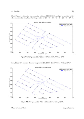
![4-1 POS Heuristic 17
mentations for Walney1 OWF [20], for a cable capacity of 10 wind turbines, can be seen in
Figures 4-1 and 4-2 respectively. The substation has an index equal to 0 and the turbines
1 to 51. The coordinates that are used, are given in Universal Transverse Mercator (UTM)
form and were converted from the corresponding latitude and longitude coordinates [21].
463 464 465 466 467 468 469 470 471
x-coordinate (km)
5985
5986
5987
5988
5989
5990
5991
5992
y-coordinate(km)
0
1
2
3
4
5
6
7
8
9
10
11
12
13
14
15
16
17
18
19
20
21
22
23
24
25
26
27
28
29
30
31
32
33
34
35
36
37
38
39
40
41
42
43
44
45
46
47
48
49
50
51
Walney1 OWF - POS1
Cable Length: 43.354 km
Capacity: 10
Cable Length: 43.354 km
Capacity: 10
Figure 4-1: ICT generated by POS1 for Walney1 OWF.
463 464 465 466 467 468 469 470 471
x-coordinate (km)
5985
5986
5987
5988
5989
5990
5991
5992
y-coordinate(km)
0
1
2
3
4
5
6
7
8
9
10
11
12
13
14
15
16
17
18
19
20
21
22
23
24
25
26
27
28
29
30
31
32
33
34
35
36
37
38
39
40
41
42
43
44
45
46
47
48
49
50
51
Walney1 OWF - POS1(-)
Cable Length: 44.272 km
Capacity: 10
Cable Length: 44.272 km
Capacity: 10
Figure 4-2: ICT generated by POS1(-) for Walney1 OWF.
As it can be seen in the two Figures, POS1(-) achieves an additional merging of the routes
Master of Science Thesis Georgios Katsouris](https://image.slidesharecdn.com/cb0cac47-df4b-46e2-bb4a-18b83a544a68-160810174410/85/Georgios_Katsouris_MSc-Thesis-35-320.jpg)
![18 Radial OWFICTP
21 − 20 − 19 − 18 − 0 and 30 − 29 − 28 − 27 − 0 by connecting turbine 18 with turbine 30, but
the solution is 2, 12% more expensive than the one calculated by POS1.
Moreover, Figures 4-1 and 4-2 reveal one clearly visible sub-optimality of POS1. As the
algorithm proceeds by examining at each iteration the maximum possible saving of merging
two routes, two specific routes that have been formed are 22 − 23 − 24 − 0 and 31 − 32 − 39 −
40−33−25−0. The merging that is achieved between these routes, from POS1, removes the
connection 24 − 0 from P and adds the connection 24 − 31. On the other hand, merging of
these two routes by connecting turbine 22 to 31 could yield a higher saving. But, for POS1
it is not possible since only connections between last and first clients are allowed.
In order to remedy this sub-optimality of POS1, Bauer and Lysgaard developed a more
sophisticated version of POS and a local search heuristic that improves sub-optimal routes,
namely POS2 (Section 4-1-2) and RouteOpt (Section 4-2) respectively.
4-1-2 POS2
POS2 follows in a great extent the logic of POS1 but it gives more freedom for merges, by
allowing not only last to first client connections but also first to first client connections.
The structure of POS2, found in [1] and adjusted according to the OWFICTP, is as follows:
POS2 (Graph (T ∪ S, P), distance d(k, u) ∀ (k, u) ∈ P, Capacity n):
1 foreach i ∈ T do si = argmins∈S{d(i, s)}
2 P ← i∈T (i, si)
3 foreach k,u ∈ T, if sk ≡ su do svku = d(k, sk) − d(k, u)
4 SV ← sorting of svku according to decreasing saving
5 repeat
6 (k,u) ← next element in SV
7 if k and u are in different routes,
8 and (k, sk) ∈ P, or k has only one neighbour in P
9 and u has only one neighbour in P,
10 and the total number of turbines in the routes containing k and u does not exceed n,
11 and (k,u) does not cross any connection in P then
12 if (k, sk) ∈ P then P ← P ((k, sk) ∪ (k, u))
13 else // k has only one neighbour in P, which is not sk
14 i ← last client in the route containing k
15 P ← P ((i, si) ∪ (k, u))
16 re-insert into SV all arcs (j, i) that were discarded earlier
17 because i had two neighbours in R
18 v ← first client of the merged route
19 w ← last client of the merged route
20 foreach z ∈ T do
21 if z has only one neighbour in P then
22 svvz ← d(w, sw) − d(v, z), and update SV accordingly
23 until end of SV is reached
24 return P
Georgios Katsouris Master of Science Thesis](https://image.slidesharecdn.com/cb0cac47-df4b-46e2-bb4a-18b83a544a68-160810174410/85/Georgios_Katsouris_MSc-Thesis-36-320.jpg)
![4-2 RouteOpt 19
The major difference compared to POS1 can be seen in line 8 where also first clients can be
examined for a possible merging with a first client of another route. In order to achieve this,
lines 14 to 22 contain the necessary adjustments of the algorithm. First, in lines 14-15, if we
assume two routes of the form k − ... − i − si and u − ... − w − sw, where si ≡ sw and the
connection that is examined corresponds to (k, u), the connection between client i and the
substation is erased and (k, u) is added in P. So, the merged route is i−...−k−u−...−w−sw.
Furthermore, it is possible that merging of routes by connecting turbine j ∈ T with turbine
i, have been examined and discarded during the sequence of iterations, since i was neither
the last nor the first client in its route. Thus, the reinsertions in lines 16-17 are necessary, in
the sense that now, turbine i is the first client in its route. Lastly, if v is the first client of the
merged route, a possible merging between v and z, where z ∈ P and has only one neighbour
in P, would erase the connection (w, sw) from P, corresponding to saving, as given in line 22.
Thus, svvz needs to be updated in SV accordingly.
Figure 4-3 presents the cable topology for Walney1 OWF, as calculated from POS2 for cable
capacity of 10 turbines. Compared to POS1 (Figure 4-1), a significant cable length reduction,
and therefore cable cost, was achieved of 6, 56%.
463 464 465 466 467 468 469 470 471
x-coordinate (m)
5985
5986
5987
5988
5989
5990
5991
5992
y-coordinate(m)
0
1
2
3
4
5
6
7
8
9
10
11
12
13
14
15
16
17
18
19
20
21
22
23
24
25
26
27
28
29
30
31
32
33
34
35
36
37
38
39
40
41
42
43
44
45
46
47
48
49
50
51
Walney1 OWF - POS2
Cable Length: 40.508 km
Capacity: 10
Cable Length: 40.508 km
Capacity: 10
Figure 4-3: ICT generated by POS2 for Walney1 OWF.
4-2 RouteOpt
RouteOpt is a local search heuristic, developed by Bauer and Lysgaard [1] that can improve
the generated sub-optimal routes of POS1 and POS2. It should be noted that firstly, the
topology is obtained by POS1 or POS2 and then RouteOpt is applied to each individual
route. As it can be seen from the results for Walney1 OWF (Figures 4-1, 4-2 and 4-3),
RouteOpt is expected to be more effective, in terms of cost reduction, for POS1 compared to
POS2, and especially for the version which includes negative savings, namely POS1(-).
Master of Science Thesis Georgios Katsouris](https://image.slidesharecdn.com/cb0cac47-df4b-46e2-bb4a-18b83a544a68-160810174410/85/Georgios_Katsouris_MSc-Thesis-37-320.jpg)
![20 Radial OWFICTP
Let r = i0 − i1 − i2 − ... − il−1 − il − ... − ik be a route, where ik ∈ S. RouteOpt examines
every feasible route rl = il−1 − ... − i2 − i1 − i0 − il − ... − ik, which is generated from r by
exchanging connection (il−1, il) with (il, i0) and where the new connection (il, i0) does not
cross any other connection in P. The improvement that is achieved by this exchange is equal
to: d(il−1, il) − d(il, i0). For every route that is generated from POS1 or POS2, RouteOpt
searches within the route for a maximum improvement, and if it is positive, the exchange is
achieved and the procedure carries on until there are no more positive improvements.
The structure of RouteOpt, found in [1] and adjusted according to the OWFICTP, is as
follows:
RouteOpt (Graph (T ∪ S, P), distance d(k, u) ∀ (k, u) ∈ P):
1 foreach route r = i0 − i1 − i2 − ... − il−1 − il − ... − ik do
2 repeat
3 sv ← maxl∈1,...,k−1{d(il−1, il) − d(il, i0)} if (il, i0) does not cross any connection
4 if sv > 0 then
5 l ← index for which d(il−1, il) − d(il, i0) = sv
6 P ← P ((il−1, il) ∪ (il, i0))
7 r ← il−1 − ... − i2 − i1 − i0 − il − ... − ik
8 until no improvement in r exists
9 return P
Figure 4-4 presents the cable topology for Walney1 OWF, after RouteOpt was applied to the
results of POS1. Compared to Figure 4-1, RouteOpt eliminated the sub-optimalities of routes
38 − 37 − 36 − 45 − 44 − 43 − 35 − 0 and 22 − 23 − 24 − 31 − 32 − 39 − 40 − 33 − 25 − 0.
463 464 465 466 467 468 469 470 471
x-coordinate (km)
5985
5986
5987
5988
5989
5990
5991
5992
y-coordinate(km)
0
1
2
3
4
5
6
7
8
9
10
11
12
13
14
15
16
17
18
19
20
21
22
23
24
25
26
27
28
29
30
31
32
33
34
35
36
37
38
39
40
41
42
43
44
45
46
47
48
49
50
51
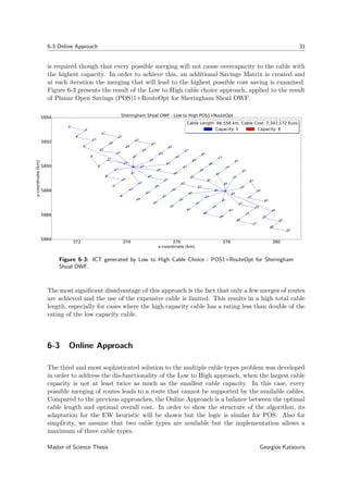
Walney1 OWF - POS1+RouteOpt
Cable Length: 41.929 km
Capacity: 10
Cable Length: 41.929 km
Capacity: 10
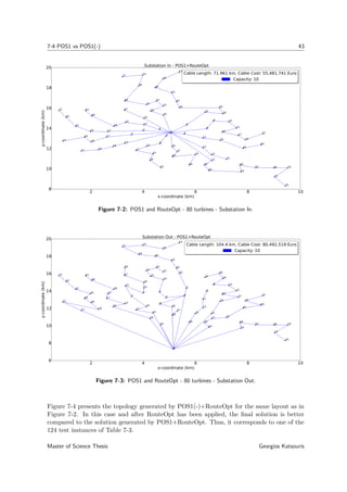
Figure 4-4: ICT generated by POS1 and RouteOpt for Walney1 OWF.
Georgios Katsouris Master of Science Thesis](https://image.slidesharecdn.com/cb0cac47-df4b-46e2-bb4a-18b83a544a68-160810174410/85/Georgios_Katsouris_MSc-Thesis-38-320.jpg)
![22 Radial OWFICTP
In this case, RouteOpt improved only route 24 − 23 − 22 − 31 − 32 − 39 − 40 − 33 − 25 − 0,
compared to Figure 4-3. Generally, the reduction in cable length that was achieved after the
implementation of RouteOpt for POS1, POS1(-) and POS2 was respectively 3.29%, 6.09%
and 0.93%. Overall, POS2+RouteOpt yields the best topology for this particular case. In
addition, it is worth mentioning that after RouteOpt implementation, POS1(-) outperformed
POS1, even if initially the solution of POS1 was better than that of POS1(-).
4-3 Test Instances
In order to verify the implementation of the algorithms and check their performance, they
are tested to the layout of three OWF, namely Barrow [22], Walney 1 [20] and Sheringham
Shoal [23], for cable capacities ranging from 5 to 10 turbines. The coordinates of the turbines
and substations, are given in UTM form and were converted from the corresponding latitude
and longitude coordinates found in [24], [21] and [25] respectively. The test instances that
are used, correspond to the ones presented by Bauer and Lysgaard [1].
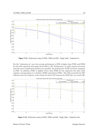
Table 4-1 lists the performance ratios of POS heuristics, for the aforementioned OWF. The
first column presents the instance (name and cable capacity) and the second column gives
the optimal solution, according to Bauer and Lysgaard [1]. They solved the test instances
to optimality with a hop indexed formulation, in order to evaluate the performance of the
heuristics. In the columns three to six, the performance of POS1, POS1+RouteOpt, POS2,
POS2+RouteOpt according to the author’s implementation, is presented respectively. In
addition, the brackets in columns 3 and 4, show the performance ratios of POS1(-) which
includes negative savings and POS1(-)+RouteOpt respectively, only for the cases for which
POS1(-) produced different results compared to POS1. Finally, the last column lists the
performance ratio of the best between all heuristics for each particular instance.
Table 4-1: Performance of POS1, POS1(-) and POS2 (+RouteOpt)
Instance opt Performance Ratio
POS1 (POS1(-)) POS1(POS1(-))+RouteOpt POS2 POS2+RouteOpt POS
Barrow
n=5 20739 1.01339 1.01339 1.00428 1.00428 1.00428
n=6 18375 1.02980 1.02974 1.02974 1.02974 1.02974
n=7 17781 1.00289 1.00289 1.00289 1.00289 1.00289
n=8 16566 1.00000 1.00000 1.00000 1.00000 1.00000
n=9 16553 1.00995 1.00995 1.00995 1.00995 1.00995
n=10 16317 1.00000 1.00000 1.00000 1.00000 1.00000
Sheringham Shoal
n=5 64828 1.04439 1.03236 1.03353 1.03236 1.03236
n=6 62031 1.08822 (1.09154) 1.07565 (1.06768) 1.04655 1.04533 1.04533
n=7 60667 1.09062 (1.12097) 1.07902 (1.04313) 1.05131 1.04769 1.04313
n=8 59836 1.08223 (1.10847) 1.07046 (1.04239) 1.02477 1.02349 1.02349
n=9 59274 1.08696 (1.12352) 1.07508 (1.06863) 1.01709 1.01581 1.01581
n=10 58960 1.09275 (1.12951) 1.08080 (1.07432) 1.02917 1.02336 1.02336
Walney 1
n=5 43539 1.02448 1.02448 1.02448 1.02448 1.02448
n=6 41587 1.05583 1.05583 1.06818 1.06818 1.05583
n=7 40789 1.06568 1.04568 1.03178 1.03178 1.03178
n=8 40242 1.08016 (1.12068) 1.05989 (1.03938) 1.04297 1.04297 1.03938
n=9 39752 1.09061 (1.11370) 1.05476 (1.04591) 1.02925 1.02297 1.02297
n=10 39541 1.09643 (1.11965) 1.06039 (1.05149) 1.02445 1.01497 1.01497
Average 1.0530 (1.06523) 1.04279 (1.03595) 1.02613 1.02445 1.02331
Georgios Katsouris Master of Science Thesis](https://image.slidesharecdn.com/cb0cac47-df4b-46e2-bb4a-18b83a544a68-160810174410/85/Georgios_Katsouris_MSc-Thesis-40-320.jpg)
![4-3 Test Instances 23
The results that were obtained, correspond to an acceptable extent with those presented by
Bauer and Lysgaard [1]. Particularly, for most instances, the results deviate for less than
1%, and only for Sheringham Shoal OWF, a few instances deviate for 3%. The differences
may occurred due to a slight deviation in the coordinates used, which can alter the sequence
of the merges and thus the overall solution. As expected, POS2 outperforms POS1 in most
instances and RouteOpt improves greatly the results of POS1 and especially POS1(-), for
which it was designed for. On average, the best between the two heuristics gives only 2.33%
more expensive solutions than the optimal.
One characteristic of POS2 that preliminary results revealed is that its performance may vary
depending on the decision of including reinsertions in the Savings matrix or not. Thus, it is
possible for the algorithm to achieve a better solution in less computation time for the case
where reinsertions are omitted (POS2*). For the particular instances of Table 4-1, POS2
and POS2* did not differentiate and therefore POS2* results were omitted. The comparison
between POS2 and POS2* can be found in Section 7-5. In general, Chapter 7 presents a
comprehensive comparison of the algorithms, regarding their performance time and cost-wise.
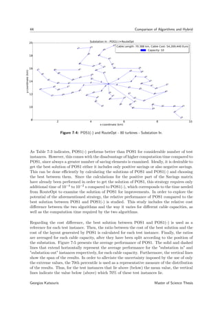
Master of Science Thesis Georgios Katsouris](https://image.slidesharecdn.com/cb0cac47-df4b-46e2-bb4a-18b83a544a68-160810174410/85/Georgios_Katsouris_MSc-Thesis-41-320.jpg)


![26 Branched OWFICTP
of cable losses between the two routes, if equal cable length for every connection is assumed,
can be found after counting the number of upstream turbines for every connection. For the
radial route, it accounts to 15 where for the branched route, the number of upstream turbines
for all connections in total is equal to 13. Thus, the branched route in this case has 15% less
losses than the radial route. It should be noted that the more branches and the closer they
take place to the substation, the greater the savings are in terms of power losses.
0
1
2
34
5
0
1
2
34
5
Figure 5-1: Radial (left) and Branched (right) routes.
Lastly, the reliability increases if a branched topology is employed. Referring again to Figure
5-1 and assuming that a cable fault occurs between turbines 2 and 3, for the radial route, the
power coming from three upstream turbines is lost. On the contrary, a cable fault in the same
connection for the branched route will only cause power from two turbines to be lost. It is
obvious that a cable fault in a connection close to the substation will have the same effect for
both designs. Therefore, the reliability in terms of cable faults is always better for branched
topologies.
On the other hand, computation time-wise, the branched solution space is essentially larger
than the radial solution space. Thus, finding the optimal solution for the branching problem
is even more difficult than the radial problem. But since the approach of the thesis is to find
near-optimal solutions in the least possible time, an heuristic algorithm will be also used for
the branching problem. This means that it is not guaranteed, that the branched topology, in
terms of cable length, will be always better than the radial topology for a particular problem,
as it is the case for the global optimum solution. Nevertheless, the undeniable advantages of
the branched over the radial topologies is a strong motivation to explore this problem.
5-2 Capacitated Minimum Spanning Tree (CMST) Problem
Finding the optimal branched solution of the OWFICTP corresponds to the well defined
CMST problem [26], which has mainly been studied for the design of minimum cost centralised
communication networks. CMST is a minimal cost spanning tree of a graph that has a
designated root node, and satisfies a capacity constraint n. The capacity constraint ensures
that all subtrees (maximal subgraphs connected to the root by a single edge) incident on
Georgios Katsouris Master of Science Thesis](https://image.slidesharecdn.com/cb0cac47-df4b-46e2-bb4a-18b83a544a68-160810174410/85/Georgios_Katsouris_MSc-Thesis-44-320.jpg)
![5-3 EW Heuristic 27
the root node have no more than n nodes. It is Non-deterministic Polynomial-time hard
(NP-hard) problem and both exact and heuristic methods have been developed [26]. In order
to fully correspond it to the OWFICTP, we need also to include the cable crossing condition.
5-3 Esau-Williams (EW) Heuristic
One of the first heuristic algorithms that was developed for the CMST problem is EW heuristic
[2]. Even if numerous additions to the algorithm have been proposed and different approaches
have been developed so far, it is considered the most efficient, regarding the computation time
and optimality of results [26]. Berzan et al. [12] used it to solve the CMST problem for large-
scale wind farms. In this section, it is adapted to approximate the near-optimal branched
topology for OWF.
EW heuristic is a Saving procedure, starting from a star tree, similar to Planar Open Savings
(POS). In each iteration the best feasible merging is performed, meaning that it yields the
largest saving. The saving svij for joining routes ri and rj by connecting nodes i and j is
defined as:
svij =
max{χi, χj} − d(i, j), if joining i and j is feasible
∞, otherwise.
(5-1)
where χi and χj represent the distance of the last clients of the routes ri and rj from the
substation respectively and d(i, j) is the distance between nodes i and j.
By using the terminology provided in Section 3-1 and the knowledge gained from POS, the
adaptation of the EW heuristic for the OWFICTP is as follows:
EW (Graph (T ∪ S, P), distance d(k, u) ∀ (k, u) ∈ P, Capacity n):
1 foreach i ∈ T do si = argmins∈S{d(i, s)}
2 P ← i∈T (i, si)
3 foreach k,u ∈ T, if sk ≡ su do svku = d(k, sk) − d(k, u)
4 SV ← k,u∈T svku
5 repeat
6 (k,u) ← maximum saving svku in SV
7 if k and u are in different routes,
8 and the total number of turbines in the routes containing k and u does not exceed n,
9 and (k,u) does not cross any connection in P then
10 i ← last client in the route containing k
11 j ← last client in the route containing u
12 P ← P ((i, si) ∪ (k, u))
13 foreach client z of the merged route do
14 if n ∈ T and svzn ∈ SV do
15 svzn ← d(j, sj) − d(z, n) and update SV acccordingly
16 delete svku from SV
17 until svku < 0
18 return P
Master of Science Thesis Georgios Katsouris](https://image.slidesharecdn.com/cb0cac47-df4b-46e2-bb4a-18b83a544a68-160810174410/85/Georgios_Katsouris_MSc-Thesis-45-320.jpg)
![Chapter 6
Multiple Cable Types Approaches
The use of multiple cable types in Offshore Wind Farms (OWF) can eliminate the pointless
use of a high capacity and thus expensive cable and contribute to the total cost saving. This
Chapter presents the three approaches that were developed for the purposes of the current
project, to solve the Offshore Wind Farm Infield Cable Topology Problem (OWFICTP) where
more than one cable type is available, in order of increasing complexity. As a reference, the
installed layout of Sheringham Shoal OWF (Figure 6-1) will be used [25]. The two cables
that are used have a capacity of 5 and 8 turbines and cost 110 and 180 e /m respectively [1].
372 374 376 378 380
x-coordinate (km)
5884
5886
5888
5890
5892
5894
y-coordinate(km)
0
24
31
1
2
3
4
5
6
7
8
9
10
11
12
13
14
15
16
17
18
19
20
21
22
23
25
26
27
28
29
30
33
34
35
36
37
41
42
43
44
49
50
51
57
0
32
38
39
40
46
47
48
53
54
55
56
59
60
61
62
63
64
66
67
68
69
70
71
72
73
74
75
76
77
78
79
80
81
82
83
84
85
86
87
88
45
52
58
65
Sheringham Shoal OWF - Installed Layout
Cable Length: 62.32 km, Cable Cost: 8,189,394 Euro
Capacity: 5 Capacity: 8
Cable Length: 62.32 km, Cable Cost: 8,189,394 Euro
Capacity: 5 Capacity: 8
Figure 6-1: Installed Layout Sheringham Shoal OWF [1].
Master of Science Thesis Georgios Katsouris](https://image.slidesharecdn.com/cb0cac47-df4b-46e2-bb4a-18b83a544a68-160810174410/85/Georgios_Katsouris_MSc-Thesis-47-320.jpg)
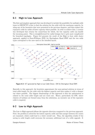

![6-4 Comparison of Approaches 33
order to achieve this, a temporary set of all the connections which assumes that the merging
has been achieved is formed. Now, it is necessary to find the connections that need to be
upgraded or downgraded (line 24-25). Especially for POS1, line 25 can be omitted since last
to first client connections are not possible to lead to a downgrade. After the saving has been
updated by subtracting the total cost of the previous solution from the cost of the assumed
solution (line 23), it is examined whether or not, the updated saving is the maximum possible.
If it is the maximum, then the merging is achieved and the assumed solution is assigned to
P. Otherwise, the algorithm continues to the next saving element.
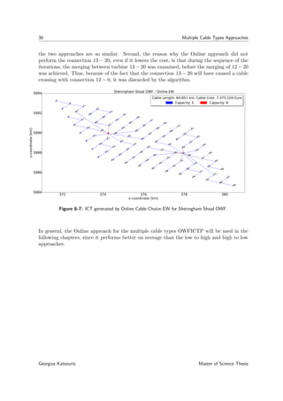
Figure 6-4 presents the result of the Online cable choice POS2 approach for Sheringham Shoal
OWF. It should be noted that for POS adaptations of the Online Approach, RouteOpt is
also applied to the connections for which the low capacity cable is used.
372 374 376 378 380
x-coordinate (m)
5884
5886
5888
5890
5892
5894
y-coordinate(m)
0
1
2
3
4
5
6
7
8
9
10
11
12
13
14
15
16
17
18
19
20
21
22
23
25
26
27
28
29
30
33
34
35
36
37
41
42
43
44
49
50
51
57
58
65
0
24
31
32
38
39
40
45
46
47
48
52
53
54
55
56
59
60
61
62
63
64
66
67
68
69
70
71
72
73
74
75
76
77
78
79
80
81
82
83
84
85
86
87
88
Sheringham Shoal OWF - Online POS2+RouteOpt
Cable Length: 63.651 km, Cable Cost: 7,300,589 Euro
Capacity: 5 Capacity: 8
Cable Length: 63.651 km, Cable Cost: 7,300,589 Euro
Capacity: 5 Capacity: 8
Figure 6-4: ICT generated by Online Cable Choice - POS2+RouteOpt for Sheringham Shoal
OWF.
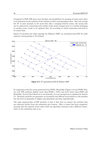
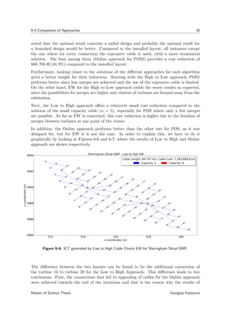
6-4 Comparison of Approaches
In order to compare the approaches, the installed and the optimal radial layout as presented
in [1], with two cable types will be used, as they can be seen in Figures 6-1 and 6-5 respec-
tively. Table 6-1 presents the performance of the three multiple cable types approaches as
implemented in POS1, POS2 and EW for Sheringham Shoal OWF with two cables of capac-
ities 5 and 8 turbines and cost 110 and 180 e /m respectively. Also, the total cost of the
solutions for the single cable type problem is included, in order to indicate the cost saving
that the use of multiple cable types can offer.
Master of Science Thesis Georgios Katsouris](https://image.slidesharecdn.com/cb0cac47-df4b-46e2-bb4a-18b83a544a68-160810174410/85/Georgios_Katsouris_MSc-Thesis-51-320.jpg)
![34 Multiple Cable Types Approaches
372 374 376 378 380
x-coordinate (km)
5884
5886
5888
5890
5892
5894
y-coordinate(km)
0
1
2
3
4
5
6
7
8
9
10
11
12
13
14
15
16
17
18
19
20
21
22
23
25
26
27
28
29
30
33
34
35
36
37
41
42
43
44
49
50
51
57
58
65
45
52
0
24
31
32
38
39
40
46
47
48
53
54
55
56
59
60
61
62
63
64
66
67
68
69
70
71
72
73
74
75
76
77
78
79
80
81
82
83
84
85
86
87
88
Sheringham Shoal OWF - Optimal Layout
Cable Length: 63.91 km, Cable Cost: 7,114,863 Euro
Capacity: 5 Capacity: 8
Cable Length: 63.91 km, Cable Cost: 7,114,863 Euro
Capacity: 5 Capacity: 8
Figure 6-5: Optimal Layout Sheringham Shoal OWF [1].
Table 6-1: Performance of Cable Choice Approaches for POS1, POS2 and EW.
Instance Performance Ratio
Optimal cost (7, 114, 863 e ) Installed cost (8, 189, 394 e )
POS1
n=5 1.035 0.899
High to Low 1.058 0.919
Low to High 1.033 0.897
Online 1.028 0.893
n=8 1.620 1.408
POS2
n=5 1.035 0.899
High to Low 1.099 0.955
Low to High 1.031 0.895
Online 1.026 0.891
n=8 1.549 1.346
EW
n=5 1.046 0.909
High to Low 1.131 0.983
Low to High 1.035 0.899
Online 1.037 0.901
n=8 1.579 1.371
As it can be seen in the Table, the best instance for each algorithm yields a solution 2.5−3.5%
more expensive than the optimal, which is considered acceptable. At this point, it should be
Georgios Katsouris Master of Science Thesis](https://image.slidesharecdn.com/cb0cac47-df4b-46e2-bb4a-18b83a544a68-160810174410/85/Georgios_Katsouris_MSc-Thesis-52-320.jpg)
![Chapter 7
Comparison of Algorithms and Hybrid
In this Chapter, the behaviour of the algorithms is examined in a wide range of test instances,
a new hybrid approach is presented and finally, recommendations are given regarding the
choice of the best algorithm for each case.
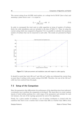
7-1 Cable Cost Model
One of the objectives of this chapter is to compare the developed algorithms for a wide
range of cable capacities. Therefore, it is necessary to incorporate their cost as related to
their capacity. The cable cost that will be used, includes cable procurement cost and cable
installation cost. It should be noted that the additional cable length that extends from the
seabed to the turbine’s transformer and back down is not taken into account. Thus, the cable
cost model is used mainly to express the relative cost difference among the available cables
and in order to allow the comparison between the solutions provided by each algorithm. By
no means can it be used to approximate the total cost of the collection system.
Several cable procurement cost models have been proposed in the literature. Some of them
present cable costs as a function of conductor cross-sectional area [27], [28]. Lundberg’s model
correlates the cable cost with the voltage level [29]. On the other hand, Zaaijer expresses
cable costs as the amount of copper and insulation material that is used [30]. Moreover, it
is mentioned in his work that the coefficients of the model were obtained after it has been
calibrated with the model of Lundberg and that Lundberg’s model has been validated with
data of existing cables.
For the purposes of the current work, Lundberg’s model is used for the cable procurement
costs by implementing the cable specifications from ABB [31]. Particularly for AC submarine
cables, their cost is given by the following equation [29]:
CostAC = Ap + Bp exp
CpSn
108
(7-1)
Master of Science Thesis Georgios Katsouris](https://image.slidesharecdn.com/cb0cac47-df4b-46e2-bb4a-18b83a544a68-160810174410/85/Georgios_Katsouris_MSc-Thesis-55-320.jpg)
![38 Comparison of Algorithms and Hybrid
where Ap, Bp and Cp are cost constants and Sn is the rated power of the cable in VA.
In order to express the cost constants in current values (Euro 2014), an average inflation rate
of 1.18 [32] for Sweden and an exchange rate of SEK to Euro of 0.1083 [33] are used. Assuming
also a voltage level of 33 kV and using the equation of the cable rated power, Sn =
√
3UnIn,
the cable procurement costs are equal to:
CostAC = 52.52 + 76.16 exp
234.35In
105
(Euro/m) (7-2)
where In is the rated current of the cable in A.
The aforementioned cost function compares well with the costs given by Dicorato et al. [34].
Lastly, Table 7-1 gives the cost of AC, XPLE 3-core, copper conductor cables according to
their cross-sectional area and rated current, as given in [31]. The cable costs are calculated
by using the rated currents of the Table in Equation 7-2.
Table 7-1: Cable procurement Costs.
Cross section (mm2) Current Rating (A) Cost (e /m)
95 300 206
120 340 221
150 375 236
185 420 256
240 480 287
300 530 316
400 590 356
500 655 406
630 715 459
800 775 521
1000 825 579
Furthermore, by incorporating cable installation costs, the relative cost difference between
the cables becomes smaller and hence, the comparison of algorithms can be made at a more
practical level. The cable installation costs, which consist of transportation and laying costs,
are usually given as a linear function of cable length and in some cases, the fixed costs are
separated by the variable costs [28], [30]. For the current comparison, a separation between
fixed and variable costs is not helpful, thus a fixed value of 365 e /m is used, as given in [34],
which compares well with the 2400 SEK/m (SEK 2003) found in [29].
7-2 Parameters
The inputs of the Offshore Wind Farm Infield Cable Topology Problem (OWFICTP), as
presented in Section 3-1, are the coordinates of turbines and substations and the capacities
and associated costs of the available cables. In order to evaluate the performance of the
algorithms, as it is explained in the following Sections, the parameters that vary are the
number of turbines, the position of the substation and the cable combinations. The same
type of wind turbine is used for all test instances.
Georgios Katsouris Master of Science Thesis](https://image.slidesharecdn.com/cb0cac47-df4b-46e2-bb4a-18b83a544a68-160810174410/85/Georgios_Katsouris_MSc-Thesis-56-320.jpg)
![7-2 Parameters 39
7-2-1 Number of Turbines
As it was shown in previous chapters, Planar Open Savings (POS) and Esau-Williams (EW)
heuristics solve the OWFICTP by starting both from the same initial solution, where the
turbines are directly connected by single lines to the closest substation. Thus, the number
of substations is irrelevant for the comparison of the performance. This allows us to use as
parameter, only the number of turbines that are connected to a single substation.
In order to choose a range for the number of turbines, the current substation ratings are taken
into account. In London Array [35], which is one of the biggest Offshore Wind Farms (OWF)
nowadays, 88 turbines of 3.6 MW are connected to a single substation. If we also consider
possible uptrends in substation ratings, 100 is the maximum number of turbines connected to
a single substation that is chosen for the current comparison. As far as the minimum number
is concerned, 30 turbines are chosen. It is highly unlikely that fewer turbines are connected to
a single substation and even if it is the case, the optimal solution could be probably calculated
by hand.
7-2-2 Position of Substation
Regarding the position of the substation, the current trend shows that in most OWF, the
substations are located within the farm, more or less in the centre of the area defined by
the turbines. This configuration yields less losses of the collection system compared to the
configuration where the substation is located outside the farm. Nevertheless, both configu-
rations are widely used and preliminary results showed that the position of substation is an
important parameter for the comparison of the algorithms.
7-2-3 Cable Capacity
Another parameter that differentiates the performance of the algorithms is the cable capacity.
The main differentiation is the choice between single or multiple cable types and additionally,
the cable capacity or the range of capacities respectively. In order to define the range of cable
capacities that will be treated, cable specifications [31] as well as layouts of existing OWF
were reviewed. The review showed that in most OWF, 5 to 10 turbines are connected in a
feeder. Hence, a range of 5 to 11 turbines is chosen for the current performance comparison
in order to account for possible upgrades in cable sizes. For the multi-cable problem, any
combination of two or three of the cable capacities in the aforementioned range could be
used. Table 7-2 shows the cable combinations that are used, which correspond to the most
practical ones and yield useful insights.
7-2-4 Selection of Turbine
The selection of turbine is not a parameter that differentiates the performance of the algo-
rithms but its purpose is to correspond cable current ratings (Table 7-1) to cable capacities,
given as number of turbines. A wind turbine with a rating of 3.6 MW is chosen, in order to
allow the use of a wide range of cables.
Master of Science Thesis Georgios Katsouris](https://image.slidesharecdn.com/cb0cac47-df4b-46e2-bb4a-18b83a544a68-160810174410/85/Georgios_Katsouris_MSc-Thesis-57-320.jpg)


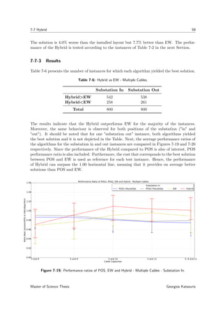
![7-7 Hybrid 55
5 and 8 5 and 9 5 and 10 5 and 11 5, 8 and 11
Cable Capacities
0.87
0.88
0.89
0.90
0.91
0.92
0.93
0.94
0.95
0.96
0.97
0.98
0.99
1.00
1.01
RatioBestsolution/Algorithm
Performance Ratio of POS1, POS2 and EW - Multiple Cables
Substation Out
POS1+RouteOpt POS2+RouteOpt EW
Figure 7-14: Performance ratios of POS1, POS2 and EW - Multiple Cables - Substation Out.
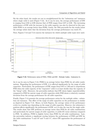
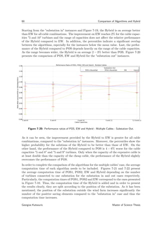
Summing up the results, the main outcome is the dependence of the algorithms’ performance
on the position of the substation. Particularly, the average performance of EW drops signifi-
cantly for the "substation out" instances compared to the "substation in" instances. Another
conclusion that can be drawn from the results is the relatively poor performance of EW when
multiple cables are used. For this reason, a hybrid approach that improves the behaviour of
EW for multiple cables is proposed in the following Section. Thus, final recommendations
regarding the use of each algorithm are made in Section 7-8, after the introduction of the
Hybrid.
7-7 Hybrid
As it was mentioned, a hybrid approach is proposed in this Section that improves the perfor-
mance of EW when more than one cable type is available. The name Hybrid denotes that it is
a combination of two algorithms, particularly POS1 and EW, and hence it concerns branched
routes.
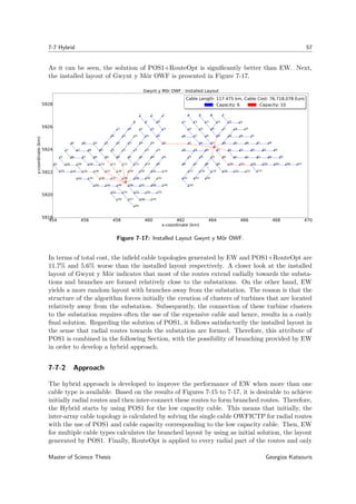
7-7-1 Motivation
The motivation to develop a hybrid by combining POS1 and EW was based on the results of
the aforementioned algorithms after tested in the layout of the Gwynt y Môr OWF [36] and
compared with its installed Infield Cable Topology (ICT) [37].
In Gwynt y Môr OWF, 160 turbines are used with a power rating of 3.6 MW. Furthermore,
two cables are used with cross sections 180 and 500 mm2 forming a branched cable topology.
The cost of these cables can be found in Table 7-1. Since a turbine of the same rating was
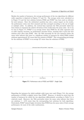
Master of Science Thesis Georgios Katsouris](https://image.slidesharecdn.com/cb0cac47-df4b-46e2-bb4a-18b83a544a68-160810174410/85/Georgios_Katsouris_MSc-Thesis-73-320.jpg)
![56 Comparison of Algorithms and Hybrid
assumed to associate the cable costs with cable capacities in terms of number of turbines in
Figure 7-1, the inter-array cables that are installed in Gwynt y Môr can withstand 6 and
10 turbines respectively. Hence, by using the coordinates of turbines and substations found
in [37] and the aforementioned cables, the OWFICTP for Gwynt y Môr is solved by using
POS1+RouteOpt and EW. The results are presented in Figures 7-15 and 7-16 respectively.
454 456 458 460 462 464 466 468 470
x-coordinate (km)
5918
5920
5922
5924
5926
5928
y-coordinate(km)
0
1 2 3 4 5 6 7
9 10 11 12 13 14 15 16
18 1922 23 24 25 26 27
29 30 3135 36 37 38 39
41 42 43 44 45 46 47 4856
58 59 60 61 62 63 64 65 66
77 78 79 80 81 82 83 84 85
96 97 98 99 100 101 102 103 104 106 107
117 118 119 120 121 122 123
133 134142
150
0
8
17 20 21
28 32 33 34
40 49 50 51 52 53 54 55
57 67 68 69 70 71 72 73 74
75 7686 87 88 89 90 91 92 93
94 95105 108 109 110 111 112 113 114
115 116124 125 126 127 128 129 130 131
132 135 136 137 138 139 140 141
143 144 145 146 147 148 149
151 152 153 154 155
156 157 158 159
160
Gwynt y Môr OWF - POS1+RouteOpt
Cable Length: 125.173 km, Cable Cost: 81,014,412 Euro
Capacity: 6 Capacity: 10
Cable Length: 125.173 km, Cable Cost: 81,014,412 Euro
Capacity: 6 Capacity: 10
Figure 7-15: ICT generated by POS1 and RouteOpt for Gwynt y Môr OWF.
454 456 458 460 462 464 466 468 470
x-coordinate (km)
5918
5920
5922
5924
5926
5928
y-coordinate(km)
0
1 2 3 4 5 6 7
9 10 11 12 13 14 15 16
18 1922 23 24 25 26 27
29 30 3135 36 37 38 39
41 42 43 44 45 46 47 4856
58 59 60 61 62 63 64 65 66
77 78 79 80 81 82 83 84 85
96 97 98 99 100 101 102 103 104 106 107
117 118 119 120 121 122 123
133 134142
150
0
8
17 20 21
28 32 33 34
40 49 50 51 52 53 54 55
57 67 68 69 70 71 72 73 74
75 7686 87 88 89 90 91 92 93
94 95105 108 109 110 111 112 113 114
115 116124 125 126 127 128 129 130 131
132 135 136 137 138 139 140 141
143 144 145 146 147 148 149
151 152 153 154 155
156 157 158 159
160
Gwynt y Môr OWF - EW
Cable Length: 130.821 km, Cable Cost: 85,670,286 Euro
Capacity: 6 Capacity: 10
Cable Length: 130.821 km, Cable Cost: 85,670,286 Euro
Capacity: 6 Capacity: 10
Figure 7-16: ICT generated by EW for Gwynt y Môr OWF.
Georgios Katsouris Master of Science Thesis](https://image.slidesharecdn.com/cb0cac47-df4b-46e2-bb4a-18b83a544a68-160810174410/85/Georgios_Katsouris_MSc-Thesis-74-320.jpg)


![66 Pipeline/Cable Crossings and Case Study
8-1-2 Transmission Lines
The main constraint for the Offshore Wind Farm Infield Cable Topology Problem (OWFICTP)
is the crossing between cables. A cable crossing could lead to excessive costs and thus, it is
strictly avoided from all algorithms that have been developed.
Moreover, the transmission lines from the substation to the onshore connection point, even
if they are not part of the collection system, are laid between the inter-array cables in the
case where the substations are centrally located in the wind farm. Therefore, an additional
constraint is imposed to the OWFICTP. Taking this into account, all algorithms are modified
to include the coordinates of the transmission lines in their inputs and they now strictly avoid
crossings between the inter-array cables and the export cables.
Figure 8-1 presents the Infield Cable Topology (ICT) for Gwynt y Môr OWF generated by
EW, which avoids the crossings with the transmission lines[37] and allows maximum double
cable connections at the turbines. Compared to Figure 7-16, the total cost is significantly
less. Hence, additional constraints to the heuristics could lead to a better final solution but
on the other hand, the computation time increases.
454 456 458 460 462 464 466 468 470
x-coordinate (km)
5918
5920
5922
5924
5926
5928
y-coordinate(km)
0
1 2 3 4 5 6 7
9 10 11 12 13 14 15 16
18 1922 23 24 25 26 27
29 30 3135 36 37 38 39
41 42 43 44 45 46 47 4856
58 59 60 61 62 63 64 65 66
77 78 79 80 81 82 83 84 85
96 97 98 99 100 101 102 103 104 106 107
117 118 119 120 121 122 123
133 134142
150
0
8
17 20 21
28 32 33 34
40 49 50 51 52 53 54 55
57 67 68 69 70 71 72 73 74
75 7686 87 88 89 90 91 92 93
94 95105 108 109 110 111 112 113 114
115 116124 125 126 127 128 129 130 131
132 135 136 137 138 139 140 141
143 144 145 146 147 148 149
151 152 153 154 155
156 157 158 159
160
Gwynt y Môr OWF - EW
Cable Length: 123.511 km, Cable Cost: 80,889,080 Euro
Capacity: 6 Capacity: 10 Transmission
Cable Length: 123.511 km, Cable Cost: 80,889,080 Euro
Capacity: 6 Capacity: 10 Transmission
Figure 8-1: ICT generated by EW for Gwynt y Môr OWF including Export Cables and Double
Switchgear.
8-2 Pipeline/Cable Crossings
In this Section, area constraints are treated that are imposed by pipelines or cables (e.g. gas
pipelines and telecommunication cables) which are laid on the seabed. In most cases, the
crossing of the inter-array cables with these pipelines cannot be entirely avoided and hence,
it is desirable to minimize the crossings and subsequently the associated costs.
Georgios Katsouris Master of Science Thesis](https://image.slidesharecdn.com/cb0cac47-df4b-46e2-bb4a-18b83a544a68-160810174410/85/Georgios_Katsouris_MSc-Thesis-84-320.jpg)
![8-3 Case study: Borssele OWF 67
The approach that was developed, aims to find a balance between the final cost of the ICT
and the minimization of crossings. Therefore, a penalty function is used that associates the
crossing with a fixed cost in monetary terms. This means that a possible crossing is considered
as one-dimensional and the dimensions of the obstacle (i.e. pipeline) are irrelevant. At this
point, it is reminded that all algorithms start from an initial solution, which connects every
turbine to the substation with a single line. Next, merges of routes are achieved that lower the
cost at each iteration. Thus, in order to force the algorithm to eliminate as much as possible
the crossings, it is required to intervene in the Savings Matrix. As it has been defined, the
cost saving svku by connecting turbine k to turbine u is equal to: svku = (d(i, s)−d(k, u))∗c,
where d(·) is the distance function between two points, s denotes the substation, i is the
turbine of the route that contains turbine k which is directly connected to the substation and
c represents the cost of the cable.
Assuming a fixed cost p for the penalty function for crossing a pipeline/cable and in order to
account for multiple crossings, the aforementioned saving is updated accordingly:
svku = (d(i, s) − d(k, u)) ∗ c + (Nis − Nku) ∗ p
where Nis and Nku represent respectively, the number of crossings of the connections i − s
and k − u with the obstacles.
The aforementioned formula is used for the calculation of the initial Savings matrix, as well
as for every point where an update in the Savings matrix is made, for all algorithms. As far
as the penalty function is concerned, the higher its value is, the more crossings are avoided.
Nevertheless, it can affect significantly the cost of the final layout and hence, reasonable values
should be used. In the following Section, a case study is presented as a representative example
of an offshore wind farm with the aforementioned area constraints.
8-3 Case study: Borssele OWF
The Borssele Wind Farm Zone (BWFZ) is located at the southern border of the Dutch
Exclusive Economic Zone (EEZ), approximately 0.5 km from the Belgian EEZ. The total area
is approximately 344 km2 [38]. The area is expected to be divided into four wind farm sites
to be used for the development of four wind farms with a total capacity of 1,400 MW. Several
operational cables and pipelines cross the wind farm zone. Furthermore, several abandoned
cables/pipelines run through the Borssele area. These pipelines and cables, together with
their safety zones (500 metres for pipelines and 750 metres for cables), are excluded from the
parcels, where turbines can be put.
Figure 8-2 presents the BWFZ according to the parcel points, found in [39]. In the Figure,
the four designated sites are depicted as well as the cables/pipelines with their safety zones.
The Wind Farm Sites at the BWFZ will be tendered in two separate tenders of which the
first will open in 2015 and the second in 2016. Wind Farm Sites I and II will be part of the
tender of 2015 whereas Wind Farm Sites III and IV will be part of the tender of the 2016.
Master of Science Thesis Georgios Katsouris](https://image.slidesharecdn.com/cb0cac47-df4b-46e2-bb4a-18b83a544a68-160810174410/85/Georgios_Katsouris_MSc-Thesis-85-320.jpg)
![68 Pipeline/Cable Crossings and Case Study
485 490 495 500 505 510
x-coordinate (km)
5710
5715
5720
5725
5730
5735
5740
y-coordinate(km)
Farland North
TAT-14
Franpipe
SeaMeWe3
Zeepipe
Borssele OWF - Wind Farm Sites
Wind Farm Sites
Wind Farm Site I
Wind Farm Site II
Wind Farm Site III
Wind Farm Site IV
Figure 8-2: Borssele OWF - Wind Farm Sites including Cables/Pipelines.
TenneT in collaboration with DNV GL proposed an array cable layout for BWFZ, where there
are two substations collecting the output of 234 x 6 MW wind turbines [40]. A voltage level of
66kV has been chosen for the collection system and 630 mm2 and 240 mm2 copper conductor
inter-array cables are used. These cables can carry the output of 13 and 8 wind turbines
respectively and their corresponding costs are 425 and 200 e /m (medium-cost estimate).
Figure 8-3 presents the proposed layout for Borssele OWF by DNV GL.
485 490 495 500 505 510
x-coordinate (km)
5710
5715
5720
5725
5730
5735
5740
y-coordinate(km)
0
1 2 3
4
5 6
7 8
9
10 1112
13 14
15
16
1718
19
20
21
22 23
24
25 26 27
28
29
30 3132
33 34
35
36
37 38
39 4041
42 43
44 45 46 47
4849 50
51
5253
54 5556
57 58
59 60
61
62
63 6465
66
6768 69
70 71 72
73 74
75
76 77
78 7980
81 8283 84
85 8687
88 89 90
9192 93 94
95 96
97 9899 100
101102103
104
105
106107108
109110
111
112113114
115
116117118
0
119
120121122
123
124125
126
127128129
130
131132
133134
135136137
138
139140141
142
143144
145
146147
148149150
151152153
154155
156157
158
159160
161162163
164165
166167168
169170171
172173
174175176
177178179
180
181182183
184185186
187188189190
191
192193194
195196197198
199
200201
202203
204205206207
208209210
211212
213214215216
217
218219
220221222
223
224225226
227228229
230231232
233234
Borssele OWF - Proposed Layout
Cable Length: 273.265 km, Cable Cost: 81,283,588 Euro
Capacity: 8 Capacity: 13
Cable Length: 273.265 km, Cable Cost: 81,283,588 Euro
Capacity: 8 Capacity: 13
Figure 8-3: ICT for Borssele OWF - DNV GL Proposal [40].
Georgios Katsouris Master of Science Thesis](https://image.slidesharecdn.com/cb0cac47-df4b-46e2-bb4a-18b83a544a68-160810174410/85/Georgios_Katsouris_MSc-Thesis-86-320.jpg)
![8-3 Case study: Borssele OWF 69
Since the coordinates of the turbines are not available, the layout of the Figure is only an
approximation of the proposed layout but nevertheless, significant effort has been put for the
maximum possible accuracy. As it can be seen, there are turbines that are located outside the
designated wind farm sites, possibly due to misinterpretation of the parcel points. However,
it does not affect the final results. Moreover, it can be observed in the Figure that crossings
with the cables/pipelines are minimized. In total, there are 26 crossings. As far as the final
cost is concerned, it accounts to approximately 81 Me . The total cost that is reported in
[40] is equal to 91 Me . The difference is due to the fact that in the current calculation, only
the cost of the cables that are laid on the seabed is included whereas most probably in [40],
the cost of the cables in the foundations and towers is included. However, rough calculations
that were made about the additional cable length, since information about the height of the
tower and the support structures are not available, agree with the aforementioned cost. It
should be noted that for the following cost comparisons, the cost of 81 Me is used. Moreover,
the cost of crossings is not included in the cost calculations. Hence, the comparison of cable
costs and number of crossings is made separately.
Next, EW and the Hybrid are used to calculate the ICT of Borssele OWF, with the same
inputs as in Figure 8-3. The resulted layouts are presented in Figures 8-4 and 8-5. For both
Figures, the algorithms without area constraints were used.
485 490 495 500 505 510
x-coordinate (km)
5710
5715
5720
5725
5730
5735
5740
y-coordinate(km)
0
1 2 3
4
5 6
7 8
9
10 1112
13 14
15
16
1718
19
20
21
22 23
24
25 26 27
28
29
30 3132
33 34
35
36
37 38
39 4041
42 43
44 45 46 47
4849 50
51
5253
54 5556
57 58
59 60
61
62
63 6465
66
6768 69
70 71 72
73 74
75
76 77
78 7980
81 8283 84
85 8687
88 89 90
9192 93 94
95 96
97 9899 100
101102103
104
105
106107108
110109
111
112113114
115
116117118
0
119
120121122
123
124125
126
127128129
130
131132
133134
135136137
138
139140141
142
143144
145
146147
148149150
151152153
154155
156157
158
159160
161162163
164165
166167168
169170171
172173
174175176
177178179
180
181182183
184185186
187188189190
191
192193194
195196197198
199
200201
202203
204205206207
208209210
211212
213214215216
217
218219
220221222
223
224225226
227228229
230231232
233234
Borssele OWF - EW (Crossing Penalty=0 Euro)
Cable Length: 332.363 km, Cable Cost: 66,472,556 Euro
Capacity: 8 Capacity: 13
Cable Length: 332.363 km, Cable Cost: 66,472,556 Euro
Capacity: 8 Capacity: 13
Figure 8-4: ICT generated by EW for Borssele OWF.
As it can be seen in Figure 8-4, the expensive cable is not used for any connection. This is not
entirely unexpected, since the price of the expensive cable is more than double of the price of
the cheap cable, whereas the range of cable capacities is relatively small (8 and 13 turbines).
Probably, if installation costs were included in the cable’s price, the result would be different.
In total, the inter-array cables cross the pipelines/cables 37 times. Regarding the cable cost,
it is 18.2% less compared to the proposed layout of Figure 8-3. Last, some cables in Figure
8-4 are laid close to each other (e.g. 59 − 0 and 63 − 0) and thus, even if it is not so clear in
the Figure, all constraints (cable capacity and inter-array cable crossings) are met.
Master of Science Thesis Georgios Katsouris](https://image.slidesharecdn.com/cb0cac47-df4b-46e2-bb4a-18b83a544a68-160810174410/85/Georgios_Katsouris_MSc-Thesis-87-320.jpg)
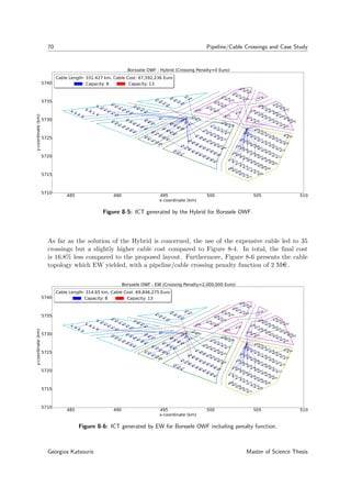
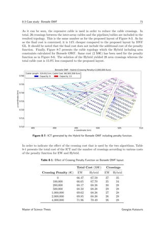


![Bibliography
[1] J. Bauer and J. Lysgaard, “The offshore wind farm array cable layout problem: A planar
open vehicle routing problem,” Journal of the Operational Research Society, 2014.
[2] L. R. Esau and K. C. Williams, “On teleprocessing system design: part ii a method for
approximating the optimal network,” IBM Systems Journal, vol. 5, no. 3, pp. 142–147,
1966.
[3] REN21, “Renewables 2013: Global status report.” http://www.ren21.net/portals/0/
documents/resources/gsr/2013/gsr2013_lowres.pdf.
[4] A. Arapogianni, J. Moccia, D. Williams, and J. Phillips, “Wind in our sails,” European
Wind Energy Asociation, pp. 1–93, 2011.
[5] IRENA, “Renewable energy cost analysis - wind power.” http://www.irena.org/
documentdownloads/publications/re_technologies_cost_analysis-wind_power.
pdf, June 2012.
[6] T. Vrana, R. Torres-Olguin, B. Liu, and T. Haileselassie, “The north sea super grid-
a technical perspective,” in AC and DC Power Transmission, 2010. ACDC. 9th IET
International Conference on, pp. 1–5, IET, 2010.
[7] E. W. E. Association et al., Wind energy-the facts: a guide to the technology, economics
and future of wind power. Routledge, 2012.
[8] M. "Gibescu and M. Ndreko, “Electrical infrastracture design for offshore wind farms.”
Offshore Wind Farm Design: Lecture Slides - Delft University of Technology, 2014.
[9] G. Quinonez-Varela, G. Ault, O. Anaya-Lara, and J. McDonald, “Electrical collector
system options for large offshore wind farms,” Renewable Power Generation, IET, vol. 1,
no. 2, pp. 107–114, 2007.
[10] S. Lumbreras and A. Ramos, “Offshore wind farm electrical design: a review,” Wind
Energy, vol. 16, no. 3, pp. 459–473, 2013.
Master of Science Thesis Georgios Katsouris](https://image.slidesharecdn.com/cb0cac47-df4b-46e2-bb4a-18b83a544a68-160810174410/85/Georgios_Katsouris_MSc-Thesis-99-320.jpg)
![82 Bibliography
[11] S. Dutta, Data mining and graph theory focused solutions to smart grid challenges. PhD
thesis, University of Illinois at Urbana-Champaign, 2013.
[12] C. Berzan, K. Veeramachaneni, J. McDermott, and U.-M. O’Reilly, “Algorithms for cable
network design on large-scale wind farms,” Rapport technique, Massachusetts Institute
of Technology, 2011.
[13] A. Hertz, O. Marcotte, A. Mdimagh, M. Carreau, and F. Welt, “Optimizing the de-
sign of a wind farm collection network,” INFOR: Information Systems and Operational
Research, vol. 50, no. 2, pp. 95–104, 2012.
[14] P. Fagerfjäll, “Optimizing wind farm layout: more bang for the buck using mixed integer
linear programming,” Master’s thesis, Chalmers University of Technology and Gothen-
burg University, 2010.
[15] S. Lumbreras and A. Ramos, “Optimal design of the electrical layout of an offshore wind
farm applying decomposition strategies,” Power Systems, IEEE Transactions on, vol. 28,
no. 2, pp. 1434–1441, 2013.
[16] D. D. Li, C. He, and Y. Fu, “Optimization of internal electric connection system of
large offshore wind farm with hybrid genetic and immune algorithm,” in Electric Util-
ity Deregulation and Restructuring and Power Technologies, 2008. DRPT 2008. Third
International Conference on, pp. 2476–2481, IEEE, 2008.
[17] F. M. González-Longatt, P. Wall, P. Regulski, and V. Terzija, “Optimal electric network
design for a large offshore wind farm based on a modified genetic algorithm approach,”
Systems Journal, IEEE, vol. 6, no. 1, pp. 164–172, 2012.
[18] G. u. Clarke and J. W. Wright, “Scheduling of vehicles from a central depot to a number
of delivery points,” Operations research, vol. 12, no. 4, pp. 568–581, 1964.
[19] G. v. Rossum et al., “Python programming language,” URL http://www. python. org,
1989.
[20] LORC, “Walney 1 Offshore Wind Farm.” http://www.lorc.dk/
offshore-wind-farms-map/walney-1. Accessed 5 March 2015.
[21] Dong Energy, “Walney 1 Offshore Wind Farm - Construction Activities.” http://www.
seafish.org/media/527826/walney_kingfisher_flyer_lres.pdf. Accessed 5 March
2015.
[22] LORC, “Barrow Offshore Wind Farm.” http://www.lorc.dk/
offshore-wind-farms-map/barrow. Accessed 5 March 2015.
[23] LORC, “Sheringham Shoal Offshore Wind Farm.” http://www.lorc.dk/
offshore-wind-farms-map/sheringham-shoal. Accessed 5 March 2015.
[24] KIS-ORCA, “Barrow Offshore Wind Farm Awareness Chart.” http://www.kis-orca.
eu/media/9284/Barrow%20OWF_LRes.pdf. Accessed 5 March 2015.
[25] KIS-ORCA, “Sheringham Shoal Offshore Wind Farm Awareness Chart.” http://
www.kis-orca.eu/media/67076/Sheringham_Shoal_OWF_LRes.pdf. Accessed 5 March
2015.
Georgios Katsouris Master of Science Thesis](https://image.slidesharecdn.com/cb0cac47-df4b-46e2-bb4a-18b83a544a68-160810174410/85/Georgios_Katsouris_MSc-Thesis-100-320.jpg)
![83
[26] A. Amberg, W. Domschke, and S. Voß, “Capacitated minimum spanning trees: Algo-
rithms using intelligent search,” 1996.
[27] J. Green, A. Bowen, L. J. Fingersh, Y. Wan, et al., “Electrical collection and transmission
systems for offshore wind power,” in Offshore technology conference, vol. 30, Offshore
Technology Conference, 2007.
[28] P. Nielsen, “Offshore wind energy projects, feasibility study guidelines,” SEAWIND-
Altener project-Feasibility Study Guidelines (EMD), 2003.
[29] S. Lundberg, “Performance comparison of wind park configurations,” tech. rep.,
Chalmers University of Technology, 2003.
[30] M. Zaaijer, Great expectations for offshore wind turbines: Emulation of wind farm de-
sign to anticipate their value for customers. PhD thesis, TU Delft, Delft University of
Technology, 2013.
[31] ABB, XLPE, “Submarine cable systems: Attachment to xlpe land cable systems-users
guide,” 2010.
[32] The World Bank, “World development indicators (2015), inflation rate - con-
sumer prices.” http://data.worldbank.org/indicator/FP.CPI.TOTL.ZG/countries/
SE?display=graph. Accessed 27 April 2015.
[33] European Central Bank, “Euro foreign exchange rates, sek vs eur.” http://www.ecb.
europa.eu/stats/exchange/eurofxref/html/eurofxref-graph-sek.en.html. Ac-
cessed 01 April 2015.
[34] M. Dicorato, G. Forte, M. Pisani, and M. Trovato, “Guidelines for assessment of invest-
ment cost for offshore wind generation,” Renewable Energy, vol. 36, no. 8, pp. 2043–2051,
2011.
[35] LORC, “London Array 1 Offshore Wind Farm.” http://www.lorc.dk/
offshore-wind-farms-map/london-array-1. Accessed 26 April 2015.
[36] LORC, “Gwynt y Môr Offshore Wind Farm.” http://www.lorc.dk/
offshore-wind-farms-map/gwynt-y-môr. Accessed 4 June 2015.
[37] KIS-ORCA, “Gwynt y Môr Offshore Wind Farm - Construction Activities.” http://www.
kis-orca.eu/media/31837/Gwynt_y_Mor_OWF_2012_LRes.pdf. Accessed 4 June 2015.
[38] Netherlands Enterprise Agency, “Borssele Wind Farm Zone - Project and Site Descrip-
tion.” http://english.rvo.nl/sites/default/files/2014/12/Borssele%20Wind%
20Farm%20Zone%20-%20Project%20and%20Site%20Description.pdf. Accessed 9 June
2015.
[39] Maarten Timmerman, “Wind Farm Sites and investigation zone around sites.” https:
//rvothema4.pleio.nl/file/download/30829692. Accessed 9 June 2015.
[40] TenneT - DNV GL, “66 kV Systems for Offshore Wind Farms.” http://www.tennet.
eu/nl/fileadmin/afbeeldingen/grid-projects/Net_iop_zee/Documentatie/T1.
_Enclosure_nr_1b_-_66_kV_systems_for_Offshore_Wind_Farms_by_DNV_GL.pdf.
Accessed 9 June 2015.
Master of Science Thesis Georgios Katsouris](https://image.slidesharecdn.com/cb0cac47-df4b-46e2-bb4a-18b83a544a68-160810174410/85/Georgios_Katsouris_MSc-Thesis-101-320.jpg)


This thesis examines optimization approaches for the design of infield cable topology for offshore wind farms. The objective is to approximate the optimal inter-array cable connections in an affordable computation time to minimize cable costs. The thesis reviews state-of-the-art collection system designs and related research, which reveals the complexity of the problem and the need for heuristic methods. Planar Open Savings and Esau-Williams heuristics are implemented and evaluated on various test instances to optimize radial and branched topologies respectively for single and multiple cable types while respecting cable capacity constraints. The results are used to develop a hybrid approach and recommendations for the best algorithm depending on the problem parameters. Additional features are included to enhance practical applicability and a case study


