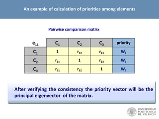
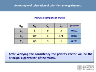
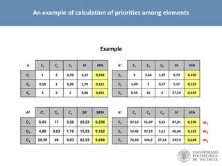
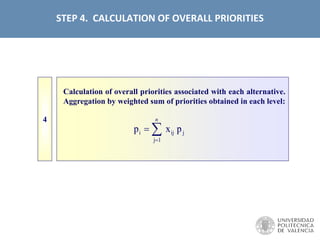
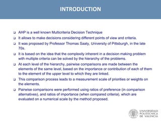
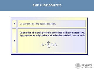
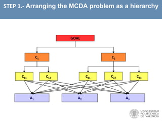
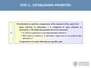
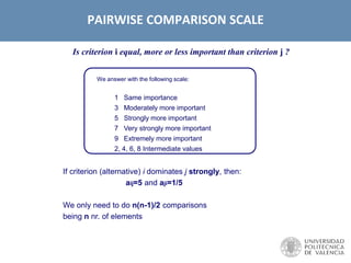
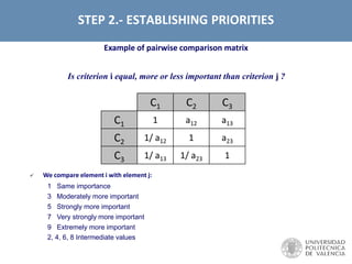
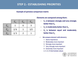
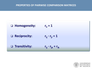
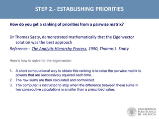
This document discusses the Analytic Hierarchy Process (AHP), a multi-criteria decision making technique. AHP allows decisions to be made by structuring multiple criteria into a hierarchy. It involves pairwise comparisons of criteria and alternatives to obtain their relative priorities. Judgments are made using a fundamental scale and priorities are derived from the principal eigenvector of the comparison matrix. Consistency of judgments is ensured by calculating a consistency ratio. The AHP provides a systematic process to integrate both subjective and objective evaluations to help decision makers select the best alternative.

1. Multicriteria Decision Analysis
MCDA
Pablo Aragonés Beltrán
and
Mónica García Melón

2. ANALYTIC HIERARCHY
PROCESS
AHP

3. MEASURING DM´S PREFERENCES
(Saaty y Peniwati, 2008)
 There are two ways to measure something about a property (or criteria).
 One is to apply an existing scale (distance in meters, weight in kg, price or costs in
Euros, etc.)
 Another is to compare the measuring object with another that is comparable to it
with respect to the property that is being measured. In this case an object serves
as a measuring unit and the other is estimated as a multiple of that unit using the
expert judgment of the DM.
 If you assign a number to something when there is no measurement scale, this
number is arbitrary and a meaningless measure.
 According to the decision process described above, first we have to measure the
importance of the criteria and in a second step measure how each alternative
satisfies the criteria.
 Finally we should combine those measures to obtain an aggregated measure
which ranks alternatives from highest to lowest preference (or priority).

4. INTRODUCTION
 AHP is a well known Multicriteria Decision Technique
 It allows to make decisions considering different points of view and criteria.
 It was proposed by Professor Thomas Saaty, University of Pittsburgh, in the late
70s.
 It is based on the idea that the complexity inherent in a decision making problem
with multiple criteria can be solved by the hierarchy of the problems.
 At each level of the hierarchy, pairwise comparisons are made between the
elements of the same level, based on the importance or contribution of each of them
to the element of the upper level to which they are linked.
 This comparison process leads to a measurement scale of priorities or weights on
the elements.
 Pairwise comparisons were performed using ratios of preference (in comparison
alternatives), and ratios of importance (when compared criteria), which are
evaluated on a numerical scale by the method proposed.

5. INTRODUCTION
 The method allows to analyze the degree of inconsistency of the judgments of the
decision maker.
 According Th Saaty, AHP is a theory of relative measurement of intangible criteria.
 AHP provides a method for measuring Decisor judgments or preferences, which in
turn are always subjective.
 Although criteria can be measured on a physical scale (full scale: kg, m, Euros,
etc.), the meaning that measure has to the decision maker is always subjective.
E.g. we can not tell if an object weighting 50 kg is very heavy or very light without
knowing in what context is this measure, for what purpose and with what other
objects you are comparing.

6. AXIOMAS BÁSICOS DEL AHP
The decision maker must be able to make comparisons and to
establish the strength of his preferences. The intensity of these
preferences must satisfy the reciprocal condition: If A is x
times more preferred than B, then B is 1 / x times more
preferred than A.
Reciprocal
comparison
The elements of a hierarchy must be comparable. The
preferences are represented by a scale of limited
comparability.
Homogeneity
When preferences are expressed, it is assumed that the
criteria are independent of the properties of the alternatives.
Independency
For the purpose of decision making, it is assumed that the
hierarchy is complete. All elements (criteria and alternatives)
of the problem are taken into account by the decision maker.
Expectations

7. 2. STEPS OF THE METHOD

8. AHP FUNDAMENTS
Arranging the MCDA problem in three hierarchical levels:
– Level:1. Main objective.
– Level 2. Criteria.
– Level 3. Alternatives.
Prioritization by pairwise comparisons of the elements of the same level:
Each criterion or alternative i is compared to each criterion or
alternative j. The following question has to be answered:
 Is criterion i equal, more or less important than criterion j ?
 With respect to criterion j, is alternative i equal, more or less preferred than
alternative j ?
Comparisons are made folowing one specific scale.
1
2

9. AHP FUNDAMENTS
Construction of the decision matrix.
Calculation of overall priorities associated with each alternative.
Aggregation by weighted sum of priorities obtained in each level:
3
4
p x pi ij
j
j

1
n

10. GOAL
C1
C11
C2
C12 C21 C22 C23
A1 A2 A3
STEP 1.- Arranging the MCDA problem as a hierarchy

11. STEP 2.- ESTABLISHING PRIORITIES
Prioritization by pairwise comparisons of the elements of the same level:
Each criterion or alternative i is compared to each criterion or
alternative j. The following question has to be answered:
 Is criterion i equal, more or less important than criterion j ?
 With respect to criterion j, is alternative i equal, more or less preferred than
alternative j ?
Comparisons are made folowing one specific scale.
2

12. PAIRWISE COMPARISON SCALE
Is criterion i equal, more or less important than criterion j ?
We answer with the following scale:
1 Same importance
3 Moderately more important
5 Strongly more important
7 Very strongly more important
9 Extremely more important
2, 4, 6, 8 Intermediate values
If criterion (alternative) i dominates j strongly, then:
aij=5 and aji=1/5
We only need to do n(n-1)/2 comparisons
being n nr. of elements

13. STEP 2.- ESTABLISHING PRIORITIES
C1 C2 C3
C1 1 a12 a13
C2 1/ a12 1 a23
C3 1/ a13 1/ a23 1
 We compare element i with element j:
1 Same importance
3 Moderately more important
5 Strongly more important
7 Very strongly more important
9 Extremely more important
2, 4, 6, 8 Intermediate values
Is criterion i equal, more or less important than criterion j ?
Example of pairwise comparison matrix

14. C1 C2 C3
C1 1 6 3
C2 1/ 6 1 1/2
C3 1/ 3 2 1
Elements are compared among them:
• C1 is between strongly and very strongly
better than C2
• C1 is moderately better than C3
• C3 is between equal and moderately
better than C2
 We compare element i with element j:
1 Same importance
3 Moderately more important
5 Strongly more important
7 Very strongly more important
9 Extremely more important
2, 4, 6, 8 Intermediate values
STEP 2.- ESTABLISHING PRIORITIES
Example of pairwise comparison matrix

15.  Homogeneity: rii = 1
 Reciprocity: rij · rji = 1
 Transitivity: rij · rjk = rik
PROPERTIES OF PAIRWISE COMPARISON MATRICES

16. How do you get a ranking of priorities from a pairwise matrix?
Dr Thomas Saaty, demonstrated mathematically that the Eigenvector
solution was the best approach
Reference : The Analytic Hierarchy Process, 1990, Thomas L. Saaty
Here’s how to solve for the eigenvector:
1. A short computational way to obtain this ranking is to raise the pairwise matrix to
powers that are successively squared each time.
2. The row sums are then calculated and normalized.
3. The computer is instructed to stop when the difference between these sums in
two consecutive calculations is smaller than a prescribed value.
STEP 2.- ESTABLISHING PRIORITIES

17. Mathematical demonstration for the Eigenvector
 Through a pairwise comparison matrix a reciprocal matrix is constructed:
aij = 1 / aij
 If the decision maker is consistent (ideal DM): aij = ai / aj
a1/a1
a2 /a1
an /a1
.
.
.
a1/a2
a2 /a2
an /a2
.
.
.
...
...
...
.
.
.
a1/an
a2 /an
an /an
.
.
.
a1
a2
an
.
.
.
= n
a1
a2
an
.
.
.
aij  aij ajk = aik
 i, j, k
(transitivity)

18.  Let A be a nxn matrix of judgements. We call Eigenvalues of A (λ1, λ2, …, λn) the
solutions to the equation: det (A-λI) = 0
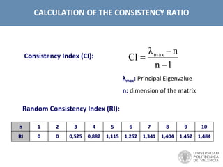
 The principal Eigenvalue (λmax) is the maximum of the Eigenvalues.
 n is the dominant Eigenvaluees of [A] and [a] is the asociated Eigenvector (ideal
case)
 If there is no consistency, the matrix of judgements becomes [R] a perturbation of
[A] and fulfills: [R] · [a] = max · [a]
( max dominant Eigenvalue  + and [a] its Eigenvector)
THE EIGENVECTOR ASSOCIATED TO THE DOMINANT EIGENVALUE
IS THE WEIGHTS VECTOR
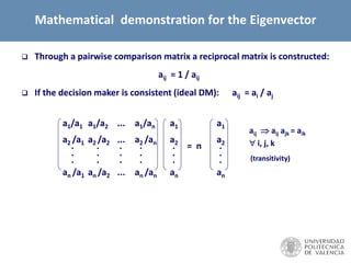
Mathematical demonstration for the Eigenvector

19. e11 C1 C2 C3 priority
C1 1 r12 r13 W1
C2 r21 1 r23 W2
C3 r31 r32 1 W3
Pairwise comparison matrix
After verifying the consistency the priority vector will be the
principal eigenvector of the matrix.
An example of calculation of priorities among elements

20. e11 C1 C2 C3 priority
C1 1 9 3 0,692
C2 1/9 1 1/3 0,077
C3 1/3 3 1 0,231
Pairwise comparison matrix
An example of calculation of priorities among elements
After verifying the consistency the priority vector will be the
principal eigenvector of the matrix.

21. A C1 C2 C3 SF SFN
C1 1 2 0,33 3,33 0,238
C2 0,50 1 0,20 1,70 0,121
C3 3 5 1 9,00 0,641
Example
A2 C1 C2 C3 SF SFN
C1 3 5,66 1,07 9,73 0,230
C2 1,60 3 0,57 5,17 0,122
C3 8,50 16 3 27,50 0,649
A3 C1 C2 C3 SF SFN
C1 9,03 17 3,20 29,23 0,230
C2 4,80 9,03 1,70 15,53 0,122
C3 25,50 48 9,03 82,53 0,648
A4 C1 C2 C3 SF SFN
C1 27,13 51,07 9,61 87,81 0,230
C2 14,42 27,13 5,11 46,66 0,122
C3 76,60 144,2 27,13 247,9 0,648
w1
w2
w3
An example of calculation of priorities among elements

22. CALCULATION OF THE CONSISTENCY RATIO
Consistency Index (CI):
1n
nλ
CI max



n 1 2 3 4 5 6 7 8 9 10
RI 0 0 0,525 0,882 1,115 1,252 1,341 1,404 1,452 1,484
λmax: Principal Eigenvalue
n: dimension of the matrix
Random Consistency Index (RI):

23. CALCULATION OF THE CONSISTENCY RATIO
Consistency Ratio (CR):
RI
CI
CR 
CI: Consistency Index
RI: Random Consistency Index
Accepted if: CR≤0,05 with n=3
CR≤0,08 with n=4
CR≤0,10 with n≥5

24. CALCULATION OF λmax
Vector B Vector CMatrix A x =
C/B Vector D=
Arithmetic mean
λmax = 3,004































1,948
0,367
0,690
0,648
0,122
0,230
1000,5000,3
200,01500,0
333,0000,21
x





















3,007
3,001
3,003
81,948/0,64
20,367/0,12
00,690/0,23
3.- Multiply matrix A original by vector B (Eigenvector) to obtain vector C.
4.- Divide vector C by vector B component by component to obtain vector D.
5.- The aritmetic mean of vector D components is the aproximate value of λmax.

25. e1 e2 e3
e1 1 2 1/3
e2 1/2 1 1/5
e3 3 5 1
λmax = 3,004  CI = (3,004-3)/(3-1) = 0,002
n = 3  RI = 0,525
CR = 0,002/0,525 = 0,004 < 0,05 
Example
CALCULATION OF THE CONSISTENCY RATIO

26. Step 3. Construction of the decision matrix
Construction of the decision matrix.
3.1 Weighting of criteria.
3.2 Assessment of alternatives.
3

27. GOAL
C1 C2
GOAL C1 C2
C1 1 r12
C2 1/r12 1
Step 3. Construction of the decision matrix.
Weighting of criteria

28. GOAL
C1 C2
GOAL C1 C2
C1 1 5
C2 1/5 1
 If criterion i dominates criterion j , e.g. with a 5 (strongly) then,
aij = 5 and aji= 1/5
 C1 is strongly more important than C2
Step 3. Construction of the decision matrix.
Weighting of criteria

29. GOAL
C1 C2
Goal C1 C2
C1 1 5
C2 1/5 1
C1 C2 media geom mgeo norm
C1 1,000 5,000 2,236 0,833
C2 0,200 1,000 0,447 0,167
Step 3. Construction of the decision matrix.
Weighting of criteria

30. C1
C11 C12
C1 C11 C12
C11 1 r11-12
C12 1/r11-12 1
C2
C21 C22 C23
C2 C21 C22 C23
C21 1 r21-22 r21-23
C22 1/r21-22 1 r22-23
C23 1/r21-23 1/r22-23 1
Step 3. Construction of the decision matrix.
Weighting of criteria

31. C1
C11 C12
C1 C11 C12
C11 1 1/3
C12 3 1
C2
C21 C22 C23
C2 C21 C22 C23
C21 1 5 1/3
C22 1/5 1 1/9
C23 3 9 1
C1 C2 media geom mgeo norm
C1 1,000 0,333 0,577 0,250
C2 3,000 1,000 1,732 0,750
C1 C2 C3 media geom mgeo norm
C1 1,000 5,000 0,333 1,186 0,265
C2 0,200 1,000 0,111 0,281 0,063
C3 3,000 9,000 1,000 3,000 0,672
Step 3. Construction of the decision matrix.
Weighting of criteria

32. GOAL
C1 C2
C11 C12
0.883 0.167
0.250 0.750
1
Local weight
0.883 0.167
0.221 0.662
1
Global weight
=
X
X C21
0.2650.044
C22
0.0630.011
C23
0.6720.112
Step 3. Construction of the decision matrix.
Weighting of criteria

33. C21 A1 A2 A3
A1 1 a12 a13
A2 1/ a12 1 a23
A3 1/ a13 1/ a23 1
C21
A1
A2 A3
Assessment of alternatives for C21
¿ Is alternative i equal, …, more important than alternative j ?
Step 3. Construction of the decision matrix.
Assessment of alternatives
 We compare element i with element j:
1 Same importance
3 Moderately more important
5 Strongly more important
7 Very strongly more important
9 Extremely more important
2, 4, 6, 8 Intermediate values

34. Assessment of alternatives for C21
C21 A1 A2 A3
A1 1 6 3
A2 1/ 6 1 1/2
A3 1/ 3 2 1
C21
A1 A2 A3
With respect to criterion C21:
• A1 is between strongly and very strongly
better than A2
• A1 is moderately better than A3
• A3 es between equal and moderately better
than A2
C1 C2 C3 media geom mgeo norm
C1 1,000 6,000 3,000 2,621 0,667
C2 0,167 1,000 0,500 0,437 0,111
C3 0,333 2,000 1,000 0,874 0,222
 We compare element i with element j:
1 Same importance
3 Moderately more important
5 Strongly more important
7 Very strongly more important
9 Extremely more important
2, 4, 6, 8 Intermediate values
Step 3. Construction of the decision matrix.
Assessment of alternatives

35. THE DECISION MATRIX
C11 C12 C21 C22 C23
WEIGHTS 0,221 0,662 0,044 0,011 0,112
A1 0,316 0,105 0,667 0,143 0,072
A2 0,386 0,258 0,111 0,429 0,649
A3 0,298 0,637 0,222 0,429 0,279

36. STEP 4. CALCULATION OF OVERALL PRIORITIES
Calculation of overall priorities associated with each alternative.
Aggregation by weighted sum of priorities obtained in each level:
4
p x pi ij
j
j

1
n

37. C11 C12 C21 C22 C23
pesos 0,221 0,662 0,044 0,011 0,112
A1 0,316 0,105 0,667 0,143 0,072
A2 0,386 0,258 0,111 0,429 0,649
A3 0,298 0,637 0,222 0,429 0,279
U(A1) = 0,221 x 0,316 + 0,662 x 0,105 + 0,044 x 0,308 + 0,011 x 0,143 + 0,112 x 0,072 = 0,163
U(A2) = 0,221 x 0,386 + 0,662 x 0,258 + 0,044 x 0,231 + 0,011 x 0,429 + 0,112 x 0,649 = 0,344
U(A3) = 0,221 x 0,298 + 0,662 x 0,637 + 0,044 x 0,308 + 0,011 x 0,429 + 0,112 x 0,279 = 0,544
STEP 4. CALCULATION OF OVERALL PRIORITIES

38. GLOBAL PRIORITIES
0,163
0,344
0,544
0,000 0,100 0,200 0,300 0,400 0,500 0,600
A1
A2
A3