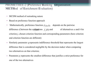
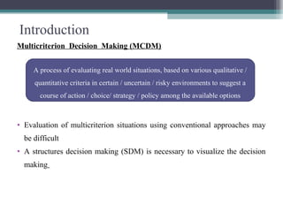
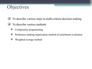
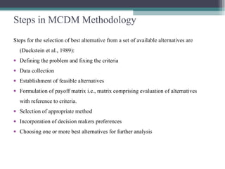
This document discusses various multi-criteria decision making (MCDM) methods. It describes the objectives and steps in MCDM methodology. Three MCDM methods are explained in detail: Compromise Programming (CP), Preference Ranking Organisation METHod of Enrichment Evaluation (PROMETHEE), and the Weighted Average Method. An example is provided to illustrate the application of each method.

1. Multi-Criteria Decision Making
Presented By : Kartik Bansal
Program : MBA

2. Introduction
Multicriterion Decision Making (MCDM)
• Evaluation of multicriterion situations using conventional approaches may
be difficult
• A structures decision making (SDM) is necessary to visualize the decision
making
A process of evaluating real world situations, based on various qualitative /
quantitative criteria in certain / uncertain / risky environments to suggest a
course of action / choice/ strategy / policy among the available options

3. Objectives
 To describe various steps in multi-criteria decision making
 To describe various methods
 Compromise programming
 Preference ranking organisation method of enrichment evaluation
 Weighted average method

4. Steps in MCDM Methodology
Steps for the selection of best alternative from a set of available alternatives are
(Duckstein et al., 1989):
• Defining the problem and fixing the criteria
• Data collection
• Establishment of feasible alternatives
• Formulation of payoff matrix i.e., matrix comprising evaluation of alternatives
with reference to criteria.
• Selection of appropriate method
• Incorporation of decision makers preferences
• Choosing one or more best alternatives for further analysis

5. MCDM Methods
MCDM methods can be classified into four groups:
1. Distance
(a) Compromise Programming (CP)
(b) Cooperative Game Theory (CGT)
(c) Technique for Order Preference by Similarity to an Ideal Solution (TOPSIS)
(d) Composite Programming (COP)
2. Outranking
(a) Preference Ranking Organisation METHod of Enrichment Evaluation (PROMETHEE)
(b) ELimination Et Choix Traduisant la REalite (ELECTRE)
3. Priority / Utility and
(a) Weighted Average Method
(b) Multi Attribute Utility Theory
(c) Analytic Hierarchy Process
4. Mixed category
(a) Multicriterion Q- Analysis -2
(b) EXPROM-2
(c) STOPROM-2
In this lecture we will discuss about compromise programming, PROMETHEE and weighted
average method

6. Compromise Programming (CP)
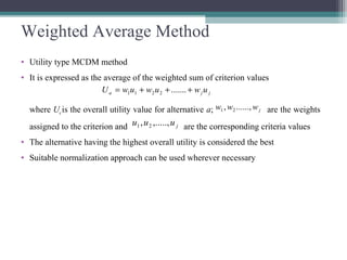
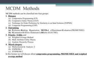
• Objective in CP: To obtain a solution that is as ‘close’ as possible to some ‘ideal’ solution in
terms of distance
• Distance measure used in Compromise Programming is the family of Lp – metrics
(1)
• Normalizing between the range [0, 1], eqn. (1) becomes,
(2)
where Lp (a) = Lp - metric for alternative a,
fj(a) = Value of criterion j for alternative a,
Mj = Maximum value of criterion j in set ,
Mj = Minimum value of criterion j in set ,
f*
j = Ideal value of criterion j,
wj = Weight assigned to the criterion j,
p = Parameter/balancing factor reflecting the attitude of the decision maker with respect to
compensation between deviations.
pJ
j
p
jj
jjp
jp
mM
aff
waL
1
1 







−
−
= ∑=
)(
)(
*
pJ
j
p
jj
p
jp affwaL
1
1






−= ∑=
)()( *

7. Compromise Programming (CP)…
• For p = 1, all deviations from are taken into account in direct proportion to their
magnitudes.
• For p = ∞, the largest deviation is the only one taken into account corresponding to
zero compensation between deviations.
Enter the number of alternatives, criteria, payoff matrix, and weight
of each criterion
Specify the parameter ; Compute - metric value
Print results
Start
Stop
Rank alternatives based on minimum - metric value
Flow chart of Compromise
Programming
methodology

8. Example: Compromise Programming (CP)
Compute - metric values of alternatives and corresponding ranking pattern for the
payoff matrix presented in Table 1 using Compromise Programming method for p =
1, 2, . Assume equal weights for each criterion. Alternatives A1 to A6 in payoff matrix
represent hydropower projects and criteria C1 to C6 correspond to man power,
Hydropower (MW), construction cost (109
$), maintenance cost (106
$), number of
villages to be evacuated and security level respectively.
Crit.
Alt.
C1 C2 C3 C4 C5 C6
A1 80 90 6 5.4 8.0 5
A2 65 58 2 9.7 1.0 1
A3 83 60 4 7.2 4.0 7
A4 40 80 10 7.5 7.0 10
A5 52 72 6 2.0 3.0 8
A6 94 96 7 3.6 5.0 6
Max/Min Min Max Min Min Min Max
Payoff Matrix

9. Example: Compromise Programming (CP)…
Solution:
Negative sign is assigned to the criterion of minimization in nature to enable to analyze
the problem uniformly in maximization perspective i.e., (-min) = max
Transformed payoff matrix
(where all criteria are made to be of maximization in nature)
Lp - metric
Crit.
Alt.
C1 C2 C3 C4 C5 C6
A1 -80 90 -6 -5.4 -8.0 5
A2 -65 58 -2 -9.7 -1.0 1
A3 -83 60 -4 -7.2 -4.0 7
A4 -40 80 -10 -7.5 -7.0 10
A5 -52 72 -6 -2.0 -3.0 8
A6 -94 96 -7 -3.6 -5.0 6
pJ
j
p
jj
jjp
jp
mM
aff
waL
1
1 







−
−
= ∑=
)(
)(
*

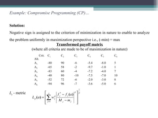
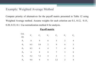
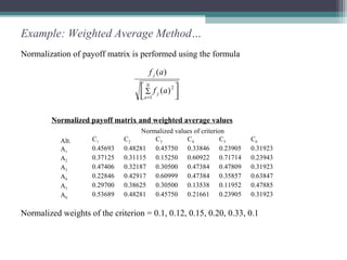
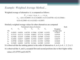
10. Example: Compromise Programming (CP)…
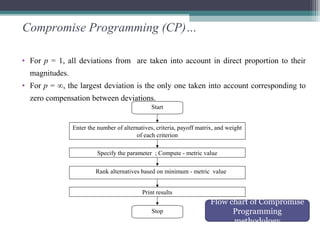
Parameters that are required for the computation of Lp - metric value
* Since there are six criteria of equal importance, normalized weight of each criterion is 1/6 i.e., 0.1666 each.
Lp - metric value of alternative A1 i.e., Lp (A1)is
Criterion C1 = =
Criterion C2 = ; Criterion C3 = ; Criterion C4 =
Criterion C5 = ; Criterion C6 =
For alternative A1, Lp - metric value for given p is
Parameters
required for each
criterion
Notation C1 C2 C3 C4 C5 C6
Maximum value Mj -40.00 96.00 -2.00 -2.00 -1.00 10.00
Minimum value mj -94.00 58.00 -10.00 -9.70 -8.00 1.00
Ideal value f*
j -40.00 96.00 -2.00 -2.00 -1.00 10.00
Weights wj 1 1 1 1 1 1
Normalized*
weights
wj 0.1666 0.1666 0.1666 0.1666 0.1666 0.1666








−−−
−−−
p
p
))00.94(00.40(
))00.80(00.40(
1666.0 p
1234074.0
p
02630526.0 p
0833.0
p
07356364.0
p
1666.0 p
09255556.0
[ ]ppppppp
1
09255556.01666.007356364.00833.002630526.01234074.0 +++++

11. Example: Compromise Programming (CP)…
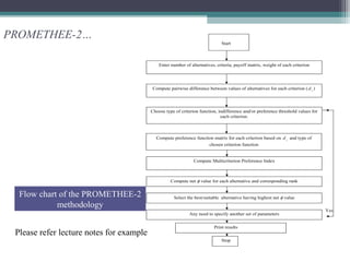
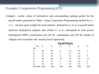
For p = 1 , L1(A1) is as follows:
= 0.56573
For p = 2 , L2(A1) is as follows:
= 0.25415
For p = 10 (approximating for ), L10(A1) is as follows:
= 0.16748
Lp - metric value of alternatives A1 to A6 and corresponding ranking pattern (values in parenthesis)
For p = 1, alternatives A5, A6,A4, A1, A2, A3 occupied ranks 1 to 6
For p = 2, these are A5, A6, A1, A3 , A4, A2
For p =∞, these are A5, A3, A6, A1, A4, A2
It is observed that first position is occupied by A5 for all the three scenarios of p = 1, 2, ∞.
[ ]1
1
09255556.01666.007356364.00833.002630526.01234074.0 +++++
[ ]2
1
222222
09255556.01666.007356364.00833.002630526.01234074.0 +++++
[ ]10
1
101010101010
09255556.01666.007356364.00833.002630526.01234074.0 +++++
Alternative p = 1 p = 2 p =
A1 0.56573 (4) 0.25415 (3) 0.16748 (4)
A2 0.57693 (6) 0.29869 (6) 0.18595 (6)
A3 0.57159 (5) 0.25512 (4) 0.16087 (2)
A4 0.49855 (3) 0.25929 (5) 0.17034 (5)
A5 0.31017 (1) 0.15171 (1) 0.10620 (1)
A6 0.47459 (2) 0.23311 (2) 0.16682 (3)
∞

12. PROMETHEE-2 (Preference Ranking Organisation
METHod of Enrichment Evaluation)
• MCDM method of outranking nature
• Based on preference function approach
• Mathematically, preference function depends on the pairwise
difference dj between the evaluations and of alternatives a and b for
criterion j, chosen criterion function and corresponding parameters (here criterion
and criterion function are different)
• Similarly parameter qjrepresents indifference threshold that represents the largest
difference that is considered negligible by the decision maker when comparing
two alternatives on that criterion;
• Parameter pj represents the smallest difference that justifies a strict preference for
one of the two alternatives
),( baPj
)(af j )(bf j

13. Types of various criterion functions
and relevant preference function
values in PROMETHEE-2
Multicriterion Preference Index, , a
weighted average of the preference
functions for all the criterion is defined as:
),( baπ

14. PROMETHEE-2…
where wj = Weight assigned to the criterion j;
= Outranking index of a in the alternatives set N;
= Outranked index of a in the alternatives set N;
= Net ranking of a in the alternatives set N;
J = Number of criteria
The alternative having the highest value is considered to be the best/suitable
)(a+
φ
)(a−
φ
)(aφ
)(aφ

15. PROMETHEE-2…
Flow chart of the PROMETHEE-2
methodology
Please refer lecture notes for example

16. Weighted Average Method
• Utility type MCDM method
• It is expressed as the average of the weighted sum of criterion values
where Ua is the overall utility value for alternative a; are the weights
assigned to the criterion and are the corresponding criteria values
• The alternative having the highest overall utility is considered the best
• Suitable normalization approach can be used wherever necessary
jja uwuwuwU +++= .......2211
jwww ......,, 21
juuu ,.....,, 21

17. Example: Weighted Average Method
Compute priority of alternatives for the payoff matrix presented in Table 12 using
Weighted Average method. Assume weights for each criterion are 0.1, 0.12, 0.15,
0.20, 0.33, 0.1. Use normalization method 4 for analysis.
Payoff matrix
Crit.
Alt.
C1 C2 C3 C4 C5 C6
A1 8 9 6 5 2 4
A2 6.5 5.8 2 9 6 3
A3 8.3 6 4 7 4 4
A4 4 8 8 7 3 8
A5 5.2 7.2 4 2 1 6
A6 9.4 9 6 3.2 2 4

18. Example: Weighted Average Method…
Normalization of payoff matrix is performed using the formula
Normalized payoff matrix and weighted average values
Normalized weights of the criterion = 0.1, 0.12, 0.15, 0.20, 0.33, 0.1



 ∑
=
N
a
j
j
af
af
1
2
)(
)(
Alt.
Normalized values of criterion
C1 C2 C3 C4 C5 C6
A1
0.45693 0.48281 0.45750 0.33846 0.23905 0.31923
A2
0.37125 0.31115 0.15250 0.60922 0.71714 0.23943
A3
0.47406 0.32187 0.30500 0.47384 0.47809 0.31923
A4
0.22846 0.42917 0.60999 0.47384 0.35857 0.63847
A5
0.29700 0.38625 0.30500 0.13538 0.11952 0.47885
A6
0.53689 0.48281 0.45750 0.21661 0.23905 0.31923

19. Example: Weighted Average Method…
Weighted average of alternative A1 is computed as follows:
Similarly weighted average values for other alternatives are computed
It is observed that the ranking pattern in the order of alternatives A1 to A6 is 4, 1, 3, 2, 6, 5.
It is observed that A2 and A4 occupied first and second positions due to their higher utility
values of 0.47978 and 0.44279.
jjA uwuwuwU +++= .......22111
35075.031923.01.023905.033.0
33846.02.045750.015.048281.012.045693.01.0(1
=×+×
+×+×+×+×=AU
Alt.
Normalized values of criterion
Weighted
average value
Rank
C1 C2 C3 C4 C5 C6
A1
0.45693 0.48281 0.45750 0.33846 0.23905 0.31923 0.35075 4
A2
0.37125 0.31115 0.15250 0.60922 0.71714 0.23943 0.47978 1
A3
0.47406 0.32187 0.30500 0.47384 0.47809 0.31923 0.41624 3
A4
0.22846 0.42917 0.60999 0.47384 0.35857 0.63847 0.44279 2
A5
0.29700 0.38625 0.30500 0.13538 0.11952 0.47885 0.23620 6
A6
0.53689 0.48281 0.45750 0.21661 0.23905 0.31923 0.33438 5