Download as PDF, PPTX


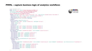
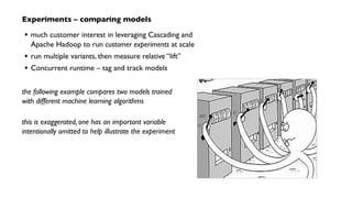
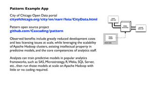
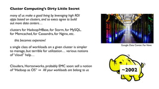
![PMML – create a model in R
## train a RandomForest model
f <- as.formula("as.factor(label) ~ .")
fit <- randomForest(f, data_train, ntree=50)
## test the model on the holdout test set
print(fit$importance)
print(fit)
predicted <- predict(fit, data)
data$predicted <- predicted
confuse <- table(pred = predicted, true = data[,1])
print(confuse)
## export predicted labels to TSV
write.table(data, file=paste(dat_folder, "sample.tsv", sep="/"),
quote=FALSE, sep="t", row.names=FALSE)
## export RF model to PMML
saveXML(pmml(fit), file=paste(dat_folder, "sample.rf.xml", sep="/"))](https://image.slidesharecdn.com/acmpattern2013-131012094851-phpapp02/85/ACM-Bay-Area-Data-Mining-Workshop-Pattern-PMML-Hadoop-6-320.jpg)

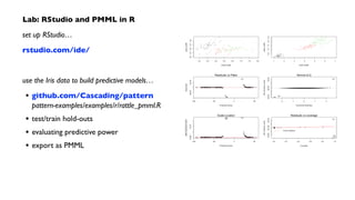
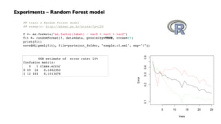
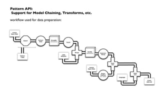
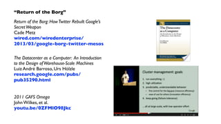
![Model: data prep based on “Iris”
library(pmml)
library(randomForest)
library(nnet)
library(XML)
library(kernlab)
## split data into test and train sets
data(iris)
iris_full <- iris
colnames(iris_full) <c("sepal_length", "sepal_width", "petal_length", "petal_width", "species")
idx <- sample(150, 100)
iris_train <- iris_full[idx,]
iris_test <- iris_full[-idx,]](https://image.slidesharecdn.com/acmpattern2013-131012094851-phpapp02/85/ACM-Bay-Area-Data-Mining-Workshop-Pattern-PMML-Hadoop-10-320.jpg)
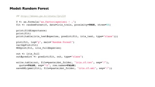
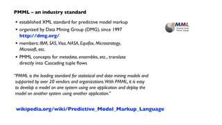
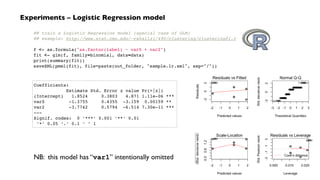
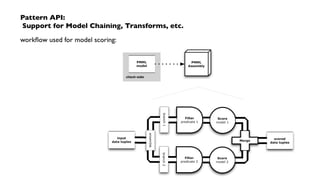
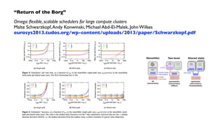
![Model: Linear Regression
## http://www2.warwick.ac.uk/fac/sci/moac/people/students/peter_cock/r/iris_lm/
f <- as.formula("sepal_length ~ .")
fit <- lm(f, data=iris_train)
print(summary(fit))
print(table(round(iris_test$sepal_length), round(predict(fit, iris_test))))
op <- par(mfrow = c(3, 2))
plot(predict(fit), main="Linear Regression")
plot(iris_full$petal_length, iris_full$petal_width, pch=21,
bg=c("red", "green3", "blue")[unclass(iris_full$species)],
main="Edgar Anderson's Iris Data", xlab="petal length", ylab="petal width")
plot(fit)
par(op)
out <- iris_full
out$predict <- predict(fit, out)
write.table(out, file=paste(dat_folder, "iris.lm_p.tsv", sep="/"),
quote=FALSE, sep="t", row.names=FALSE)
saveXML(pmml(fit), file=paste(dat_folder, "iris.lm_p.xml", sep="/"))](https://image.slidesharecdn.com/acmpattern2013-131012094851-phpapp02/85/ACM-Bay-Area-Data-Mining-Workshop-Pattern-PMML-Hadoop-12-320.jpg)
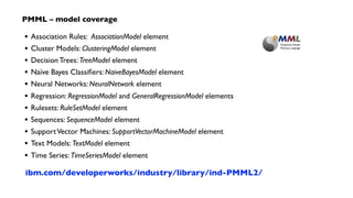
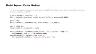
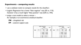
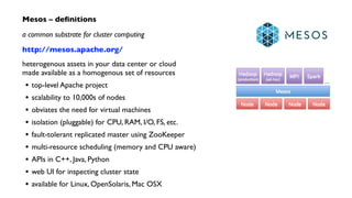
![Model: Neural Network
## http://statisticsr.blogspot.com/2008/10/notes-for-nnet.html
samp <- c(sample(1:50,25), sample(51:100,25), sample(101:150,25))
ird <- data.frame(rbind(iris3[,,1], iris3[,,2], iris3[,,3]),
species=factor(c(rep("setosa",50), rep("versicolor", 50), rep("virginica", 50))))
f <- as.formula("species ~ .")
fit <- nnet(f, data=ird, subset=samp, size=2, rang=0.1, decay=5e-4, maxit=200)
print(fit)
print(summary(fit))
print(table(ird$species[-samp], predict(fit, ird[-samp,], type = "class")))
out <- ird
out$predict <- predict(fit, ird, type="class")
write.table(out, file=paste(dat_folder, "iris.nn.tsv", sep="/"),
quote=FALSE, sep="t", row.names=FALSE)
saveXML(pmml(fit), file=paste(dat_folder, "iris.nn.xml", sep="/"))](https://image.slidesharecdn.com/acmpattern2013-131012094851-phpapp02/85/ACM-Bay-Area-Data-Mining-Workshop-Pattern-PMML-Hadoop-13-320.jpg)
![Model: K-Means Clustering
## http://mkseo.pe.kr/stats/?p=15
ds <- iris_full[,-5]
fit <- kmeans(ds, 3)
print(fit)
print(summary(fit))
print(table(fit$cluster, iris_full$species))
op <- par(mfrow = c(1, 1))
plot(iris_full$sepal_length, iris_full$sepal_width, pch = 23,
bg = c("blue", "red", "green")[fit$cluster], main="K-Means Clustering")
points(fit$centers[,c(1, 2)], col=1:3, pch=8, cex=2)
par(op)
out <- iris_full
out$predict <- fit$cluster
write.table(out, file=paste(dat_folder, "iris.kmeans.tsv", sep="/"),
quote=FALSE, sep="t", row.names=FALSE)
saveXML(pmml(fit), file=paste(dat_folder, "iris.kmeans.xml", sep="/"))](https://image.slidesharecdn.com/acmpattern2013-131012094851-phpapp02/85/ACM-Bay-Area-Data-Mining-Workshop-Pattern-PMML-Hadoop-14-320.jpg)
![Model: Hierarchical Clustering
## http://mkseo.pe.kr/stats/?p=15
i = as.matrix(iris_full[,-5])
fit <- hclust(dist(i), method = "average")
initial <- tapply(i, list(rep(cutree(fit, 3), ncol(i)), col(i)), mean)
dimnames(initial) <- list(NULL, dimnames(i)[[2]])
kls = cutree(fit, 3)
print(fit)
print(table(iris_full$species, kls))
op <- par(mfrow = c(1, 1))
plclust(fit, main="Hierarchical Clustering")
par(op)
out <- iris_full
out$predict <- kls
write.table(out, file=paste(dat_folder, "iris.hc.tsv", sep="/"),
quote=FALSE, sep="t", row.names=FALSE)
saveXML(pmml(fit, data=iris, centers=initial),
file=paste(dat_folder, "iris.hc.xml", sep="/"))](https://image.slidesharecdn.com/acmpattern2013-131012094851-phpapp02/85/ACM-Bay-Area-Data-Mining-Workshop-Pattern-PMML-Hadoop-15-320.jpg)


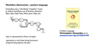

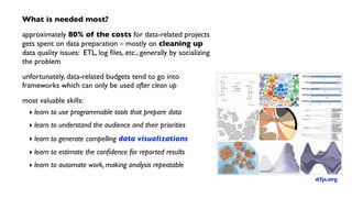
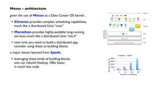
![WordCount – Cascading app in Java
Document
Collection
String docPath = args[ 0 ];
String wcPath = args[ 1 ];
Properties properties = new Properties();
AppProps.setApplicationJarClass( properties, Main.class );
HadoopFlowConnector flowConnector = new HadoopFlowConnector( properties );
// create source and sink taps
Tap docTap = new Hfs( new TextDelimited( true, "t" ), docPath );
Tap wcTap = new Hfs( new TextDelimited( true, "t" ), wcPath );
// specify a regex to split "document" text lines into token stream
Fields token = new Fields( "token" );
Fields text = new Fields( "text" );
RegexSplitGenerator splitter = new RegexSplitGenerator( token, "[ [](),.]" );
// only returns "token"
Pipe docPipe = new Each( "token", text, splitter, Fields.RESULTS );
// determine the word counts
Pipe wcPipe = new Pipe( "wc", docPipe );
wcPipe = new GroupBy( wcPipe, token );
wcPipe = new Every( wcPipe, Fields.ALL, new Count(), Fields.ALL );
// connect the taps, pipes, etc., into a flow
FlowDef flowDef = FlowDef.flowDef().setName( "wc" )
.addSource( docPipe, docTap )
.addTailSink( wcPipe, wcTap );
// write a DOT file and run the flow
Flow wcFlow = flowConnector.connect( flowDef );
wcFlow.writeDOT( "dot/wc.dot" );
wcFlow.complete();
Tokenize
M
GroupBy
token
R
Count
Word
Count](https://image.slidesharecdn.com/acmpattern2013-131012094851-phpapp02/85/ACM-Bay-Area-Data-Mining-Workshop-Pattern-PMML-Hadoop-36-320.jpg)
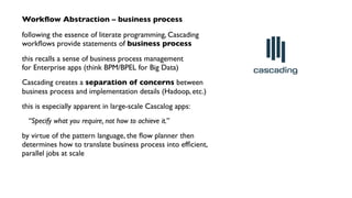
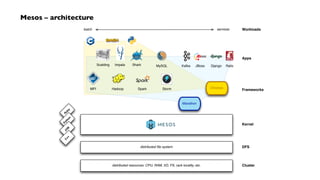
![WordCount – generated flow diagram
Document
Collection
Tokenize
[head]
M
GroupBy
token
R
Hfs['TextDelimited[['doc_id', 'text']->[ALL]]']['data/rain.txt']']
map
[{2}:'doc_id', 'text']
[{2}:'doc_id', 'text']
Each('token')[RegexSplitGenerator[decl:'token'][args:1]]
[{1}:'token']
[{1}:'token']
GroupBy('wc')[by:['token']]
Every('wc')[Count[decl:'count']]
[{2}:'token', 'count']
[{1}:'token']
Hfs['TextDelimited[[UNKNOWN]->['token', 'count']]']['output/wc']']
[{2}:'token', 'count']
[{2}:'token', 'count']
[tail]
reduce
wc[{1}:'token']
[{1}:'token']
Count
Word
Count](https://image.slidesharecdn.com/acmpattern2013-131012094851-phpapp02/85/ACM-Bay-Area-Data-Mining-Workshop-Pattern-PMML-Hadoop-37-320.jpg)
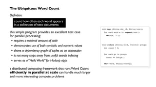
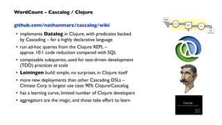
![WordCount – Cascalog / Clojure
Document
Collection
(ns impatient.core
(:use [cascalog.api]
[cascalog.more-taps :only (hfs-delimited)])
(:require [clojure.string :as s]
[cascalog.ops :as c])
(:gen-class))
(defmapcatop split [line]
"reads in a line of string and splits it by regex"
(s/split line #"[[](),.)s]+"))
(defn -main [in out & args]
(?<- (hfs-delimited out)
[?word ?count]
((hfs-delimited in :skip-header? true) _ ?line)
(split ?line :> ?word)
(c/count ?count)))
; Paul Lam
; github.com/Quantisan/Impatient
Tokenize
M
GroupBy
token
R
Count
Word
Count](https://image.slidesharecdn.com/acmpattern2013-131012094851-phpapp02/85/ACM-Bay-Area-Data-Mining-Workshop-Pattern-PMML-Hadoop-38-320.jpg)
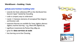
![WordCount – Scalding / Scala
Document
Collection
import com.twitter.scalding._
class WordCount(args : Args) extends Job(args) {
Tsv(args("doc"),
('doc_id, 'text),
skipHeader = true)
.read
.flatMap('text -> 'token) {
text : String => text.split("[ [](),.]")
}
.groupBy('token) { _.size('count) }
.write(Tsv(args("wc"), writeHeader = true))
}
Tokenize
M
GroupBy
token
R
Count
Word
Count](https://image.slidesharecdn.com/acmpattern2013-131012094851-phpapp02/85/ACM-Bay-Area-Data-Mining-Workshop-Pattern-PMML-Hadoop-40-320.jpg)
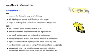
![WordCount – Apache Hive
Document
Collection
CREATE TABLE text_docs (line STRING);
LOAD DATA LOCAL INPATH 'data/rain.txt'
OVERWRITE INTO TABLE text_docs
;
SELECT
word, COUNT(*)
FROM
(SELECT
split(line, 't')[1] AS text
FROM text_docs
) t
LATERAL VIEW explode(split(text, '[ ,.()]')) lTable AS
word
GROUP BY word
;
Tokenize
M
GroupBy
token
R
Count
Word
Count](https://image.slidesharecdn.com/acmpattern2013-131012094851-phpapp02/85/ACM-Bay-Area-Data-Mining-Workshop-Pattern-PMML-Hadoop-42-320.jpg)
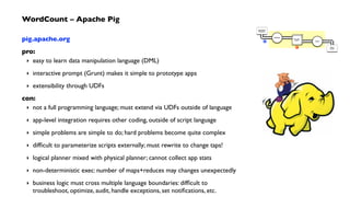
![WordCount – Apache Pig
Document
Collection
docPipe = LOAD '$docPath' USING PigStorage('t', 'tagsource')
AS (doc_id, text);
docPipe = FILTER docPipe BY doc_id != 'doc_id';
-- specify regex to split "document" text lines into token stream
tokenPipe = FOREACH docPipe
GENERATE doc_id, FLATTEN(TOKENIZE(text, ' [](),.')) AS token;
tokenPipe = FILTER tokenPipe BY token MATCHES 'w.*';
-- determine the word counts
tokenGroups = GROUP tokenPipe BY token;
wcPipe = FOREACH tokenGroups
GENERATE group AS token, COUNT(tokenPipe) AS count;
-- output
STORE wcPipe INTO '$wcPath' USING PigStorage('t', 'tagsource');
EXPLAIN -out dot/wc_pig.dot -dot wcPipe;
Tokenize
M
GroupBy
token
R
Count
Word
Count](https://image.slidesharecdn.com/acmpattern2013-131012094851-phpapp02/85/ACM-Bay-Area-Data-Mining-Workshop-Pattern-PMML-Hadoop-44-320.jpg)

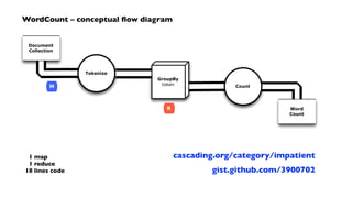
![Pattern – score a model, within an app
public static void main( String[] args ) throws RuntimeException {
String inputPath = args[ 0 ];
String classifyPath = args[ 1 ];
// set up the config properties
Properties properties = new Properties();
AppProps.setApplicationJarClass( properties, Main.class );
HadoopFlowConnector flowConnector = new HadoopFlowConnector( properties );
// create source and sink taps
Tap inputTap = new Hfs( new TextDelimited( true, "t" ), inputPath );
Tap classifyTap = new Hfs( new TextDelimited( true, "t" ), classifyPath );
// handle command line options
OptionParser optParser = new OptionParser();
optParser.accepts( "pmml" ).withRequiredArg();
OptionSet options = optParser.parse( args );
// connect the taps, pipes, etc., into a flow
FlowDef flowDef = FlowDef.flowDef().setName( "classify" )
.addSource( "input", inputTap )
.addSink( "classify", classifyTap );
if( options.hasArgument( "pmml" ) ) {
String pmmlPath = (String) options.valuesOf( "pmml" ).get( 0 );
PMMLPlanner pmmlPlanner = new PMMLPlanner()
.setPMMLInput( new File( pmmlPath ) )
.retainOnlyActiveIncomingFields()
.setDefaultPredictedField( new Fields( "predict", Double.class ) ); // default value if missing from the model
flowDef.addAssemblyPlanner( pmmlPlanner );
}
// write a DOT file and run the flow
Flow classifyFlow = flowConnector.connect( flowDef );
classifyFlow.writeDOT( "dot/classify.dot" );
classifyFlow.complete();
}](https://image.slidesharecdn.com/acmpattern2013-131012094851-phpapp02/85/ACM-Bay-Area-Data-Mining-Workshop-Pattern-PMML-Hadoop-50-320.jpg)


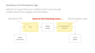
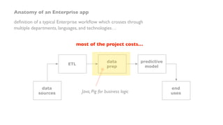
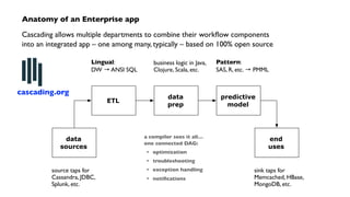
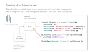
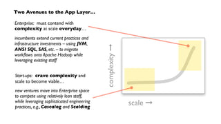
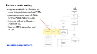
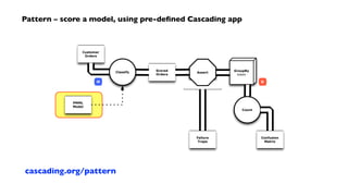
The document outlines a workshop on PMML (Predictive Model Markup Language) and Cascading, focusing on their application in machine learning and data mining. It covers topics such as model scoring, industry practices, and offers practical lab sessions utilizing R for creating and exporting models in PMML format. The content emphasizes the importance of PMML as an industry standard and the role of Cascading in integrating diverse data workflows across departments.