SlideShare a Scribd company logo
1 of 28
Supervised Machine
Learning in R
Babu Priyavrat
Supervised Machine learning
• Formal boring definition - Supervised learning task of inferring a function from
labeled training data. The training data consist of a set of training examples. In
supervised learning, each example is a pair consisting of an input object (typically
a vector) and a desired output value (also called the supervisory signal).
• Layman term – Make computers learn from experience
• Task Driven
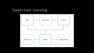
Supervised Learning
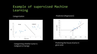
Example of supervised Machine
Learning
Categorization
Categorizing whether tumor is
malignant or benign
Prediction (Regression)
Predicting the house of price in
given area
What is R?
• R is a language and environment for statistical computing and graphics
developed at Bell Laboratories (formerly AT&T, now Lucent Technologies) by
John Chambers and colleagues.
R basics
• Assignment
• Data types
• Accessing directories
• Reading a CSV file
• Accessing the data of CSV file
• Listing all variables
• Getting the type of variable
• Arithmetic functions
• Difference between names and attributes
R Basics
• Assignment :
babu<- c(3,5,7,9)
• Accessing variables:
babu[1] - > 3
• Data types: list, double,character,integer
String example : b <- c("hello","there")
Logiical: a = TRUE
Converting character to integer = factor
• Getting the current directory: getwd()
• tree <-
read.csv(file="trees91.csv",header=TRUE,
sep=",");
names(tree); summary(tree); tree[1]; tree$C
• Listing all variables: ls()
• Type of variables:
typeof(babu)
typeof(list)
• Arithmetic functions: mean(babu)
• Converting array into table: table()
R Basics
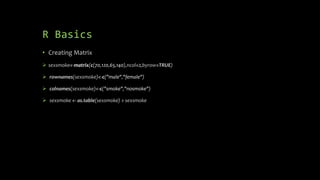
• Creating Matrix
 sexsmoke<-matrix(c(70,120,65,140),ncol=2,byrow=TRUE)
 rownames(sexsmoke)<-c("male","female")
 colnames(sexsmoke)<-c("smoke","nosmoke")
 sexsmoke <- as.table(sexsmoke) > sexsmoke
How is Supervised Learning Achieved?
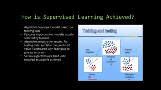
• Algorithm develops it model based on
training data
• Features important for model is usually
selected by humans
• Algorithm predicts the results for
testing data and later the predicted
value is compared with real value to
give us accuracy.
• Several algorithms are tried until
required accuracy is achieved
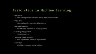
Basic steps in Machine Learning
• Questions
• Start with a general question and making the question concrete?
• Input Data
• Cleaning Data , Pre-processing & Partitioning
• Features Selection
• What features are important for my algorithm?
• Selecting the algorithm
• What best suits me
• Selecting the parameters
• Each algorithm has certain set of parameters
• Evaluation
• Checking the accuracy after prediction
Input Data
• Cleaning
• input<- read.csv("pml-training.csv", na.strings = c("NA", "#DIV/0!", ""))
• input =input[,colSums(is.na(input)) == 0]
• standardization
standardhousing <-(housing$Home.Value-
mean(housing$Home.Value))/(sd(housing$Home.Value))
• Removing Near Zero covariates
nsvCol =nearZeroVar(housing)
Input Data
• Partitioning the Data is done early
• Thumbs of Rule of partitioning
• 40% -testing, 60% - training or 70% -training 30% -testing for medium data sets
• 20%-testing, 20%-validation, 60%- validation
• R Code for partitioning:
• library(caret)
• set.seed(11051985)
• inTrain <- createDataPartition(y=input$classe, p=0.70, list=FALSE)
• training <- input[inTrain,]
• testing <- input[-inTrain,]
Features Selection
• Done by understanding the data
• Plotting
• Developing a Decision Tree
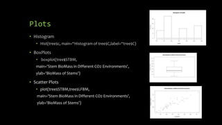
Plots
• Histogram
• Hist(tree$c, main=“Histogram of tree$C,label=“tree$C)
• BoxPlots
• boxplot(tree$STBM,
main='Stem BioMass in Different CO2 Environments',
ylab='BioMass of Stems')
• Scatter Plots
• plot(tree$STBM,tree$LFBM,
main='Stem BioMass in Different CO2 Environments',
ylab='BioMass of Stems')
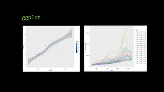
ggplot
ggplot
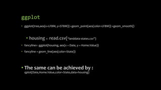
• ggplot(tree,aes(x=LFBM, y=STBM)) +geom_point(aes(color=LFBM)) +geom_smooth()
• housing <- read.csv(“landdata-states.csv”)
• fancyline<- ggplot(housing, aes(x = Date, y = Home.Value))
• fancyline + geom_line(aes(color=State))
• The same can be achieved by :
qplot(Date,Home.Value,color=State,data=housing)
ggplot
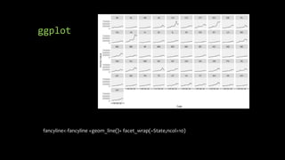
fancyline<-fancyline +geom_line()+ facet_wrap(~State,ncol=10)
Creating a Decision Tree
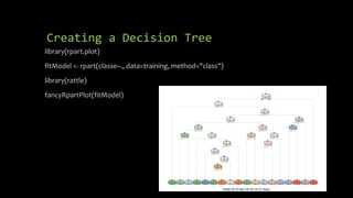
library(rpart.plot)
fitModel <- rpart(classe~., data=training, method="class")
library(rattle)
fancyRpartPlot(fitModel)
Selecting the Algorithm
• Linear Regression
• Decision Tree
• Random Forest
• Boosting
Linear Regression
• Linear Regression is the simplest machine algorithm and it is
usually used to identify if any correlation exists.
R code:
Modelfit <-
train(survived~Class,data=training,method=“lm”)
Predictions <- predict(Modelfit,newdata=testing)
• More than one variables can be used for linear regression
R code:
Modelfit <-
train(survived~Class+Age,data=training,method=“lm”)
Predictions <- predict(Modelfit,newdata=testing)
Decision Tree
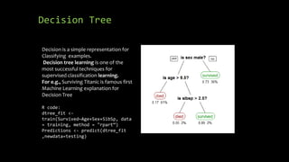
Decision is a simple representation for
Classifying examples.
Decision tree learning is one of the
most successful techniques for
supervised classification learning.
For e.g., Surviving Titanic is famous first
Machine Learning explanation for
Decision Tree
R code:
dtree_fit <-
train(Survived~Age+Sex+SibSp, data
= training, method = "rpart“)
Predictions <- predict(dtree_fit
,newdata=testing)
Random Forest
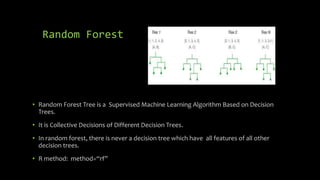
• Random Forest Tree is a Supervised Machine Learning Algorithm Based on Decision
Trees.
• It is Collective Decisions of Different Decision Trees.
• In random forest, there is never a decision tree which have all features of all other
decision trees.
• R method: method=“rf”
Boosting
• Form a large set of simple features
• Initialize weights for training images
• For T rounds
• Normalize the weights
• For available features from the set, train a classifier using a single feature and evaluate the
training error
• Choose the classifier with the lowest error
• Update the weights of the training images: increase if classified wrongly by this classifier,
decrease if correctly
• Form the final strong classifier as the linear combination of the T classifiers
(coefficient larger if training error is small)
• Method:”gmb”
Cross Validation
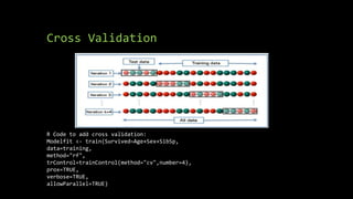
R Code to add cross validation:
Modelfit <- train(Survived~Age+Sex+SibSp,
data=training,
method="rf",
trControl=trainControl(method="cv",number=4),
prox=TRUE,
verbose=TRUE,
allowParallel=TRUE)
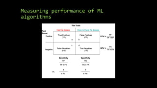
Measuring performance of ML
algorithms
Calculating Accuracy
• confMatrix<- confusionMatrix(predictions, testing$Survived)
## Confusion Matrix and Statistics
##
## Reference
## Prediction 0 1
## 0 506 88
## 1 43 254
##
## Accuracy : 0.853
## 95% CI : (0.828, 0.8756)
## No Information Rate : 0.6162
## P-Value [Acc > NIR] : < 2.2e-16
##
## Kappa : 0.6813
## Mcnemar's Test P-Value : 0.0001209
##
## Sensitivity : 0.9217
## Specificity : 0.7427
## Pos Pred Value : 0.8519
## Neg Pred Value : 0.8552
## Prevalence : 0.6162
## Detection Rate : 0.5679
## Detection Prevalence : 0.6667
## Balanced Accuracy : 0.8322
##
## 'Positive' Class : 0
Participate in Machine Learning
Competitions
http://www.kaggle.com/
Question & Answers

More Related Content

What's hot

Introduction to-machine-learning
Introduction to-machine-learningIntroduction to-machine-learning
Introduction to-machine-learningBabu Priyavrat
 
Deep Learning for Recommender Systems RecSys2017 Tutorial
Deep Learning for Recommender Systems RecSys2017 Tutorial Deep Learning for Recommender Systems RecSys2017 Tutorial
Deep Learning for Recommender Systems RecSys2017 Tutorial Alexandros Karatzoglou
 
Deep Learning With Neural Networks
Deep Learning With Neural NetworksDeep Learning With Neural Networks
Deep Learning With Neural NetworksAniket Maurya
 
Introduction to text classification using naive bayes
Introduction to text classification using naive bayesIntroduction to text classification using naive bayes
Introduction to text classification using naive bayesDhwaj Raj
 
Machine Learning
Machine LearningMachine Learning
Machine LearningKumar P
 
Deep Learning Tutorial
Deep Learning TutorialDeep Learning Tutorial
Deep Learning TutorialAmr Rashed
 
Model selection and cross validation techniques
Model selection and cross validation techniquesModel selection and cross validation techniques
Model selection and cross validation techniquesVenkata Reddy Konasani
 
Automated Machine Learning
Automated Machine LearningAutomated Machine Learning
Automated Machine Learningsafa cimenli
 
Multilayer perceptron
Multilayer perceptronMultilayer perceptron
Multilayer perceptronomaraldabash
 
Backpropagation And Gradient Descent In Neural Networks | Neural Network Tuto...
Backpropagation And Gradient Descent In Neural Networks | Neural Network Tuto...Backpropagation And Gradient Descent In Neural Networks | Neural Network Tuto...
Backpropagation And Gradient Descent In Neural Networks | Neural Network Tuto...Simplilearn
 
Neural Networks: Multilayer Perceptron
Neural Networks: Multilayer PerceptronNeural Networks: Multilayer Perceptron
Neural Networks: Multilayer PerceptronMostafa G. M. Mostafa
 
Machine Learning
Machine LearningMachine Learning
Machine LearningVivek Garg
 
Convolution Neural Network (CNN)
Convolution Neural Network (CNN)Convolution Neural Network (CNN)
Convolution Neural Network (CNN)Basit Rafiq
 
Deep Learning - CNN and RNN
Deep Learning - CNN and RNNDeep Learning - CNN and RNN
Deep Learning - CNN and RNNAshray Bhandare
 
Feature Engineering
Feature Engineering Feature Engineering
Feature Engineering odsc
 

What's hot (20)

Introduction to-machine-learning
Introduction to-machine-learningIntroduction to-machine-learning
Introduction to-machine-learning
 
Deep Learning for Recommender Systems RecSys2017 Tutorial
Deep Learning for Recommender Systems RecSys2017 Tutorial Deep Learning for Recommender Systems RecSys2017 Tutorial
Deep Learning for Recommender Systems RecSys2017 Tutorial
 
Deep Learning With Neural Networks
Deep Learning With Neural NetworksDeep Learning With Neural Networks
Deep Learning With Neural Networks
 
Introduction to text classification using naive bayes
Introduction to text classification using naive bayesIntroduction to text classification using naive bayes
Introduction to text classification using naive bayes
 
Machine Learning
Machine LearningMachine Learning
Machine Learning
 
Deep Learning Tutorial
Deep Learning TutorialDeep Learning Tutorial
Deep Learning Tutorial
 
Introduction to Transformer Model
Introduction to Transformer ModelIntroduction to Transformer Model
Introduction to Transformer Model
 
Model selection and cross validation techniques
Model selection and cross validation techniquesModel selection and cross validation techniques
Model selection and cross validation techniques
 
SVM
SVM SVM
SVM
 
Automated Machine Learning
Automated Machine LearningAutomated Machine Learning
Automated Machine Learning
 
Multilayer perceptron
Multilayer perceptronMultilayer perceptron
Multilayer perceptron
 
Backpropagation And Gradient Descent In Neural Networks | Neural Network Tuto...
Backpropagation And Gradient Descent In Neural Networks | Neural Network Tuto...Backpropagation And Gradient Descent In Neural Networks | Neural Network Tuto...
Backpropagation And Gradient Descent In Neural Networks | Neural Network Tuto...
 
Neural Networks: Multilayer Perceptron
Neural Networks: Multilayer PerceptronNeural Networks: Multilayer Perceptron
Neural Networks: Multilayer Perceptron
 
Densenet CNN
Densenet CNNDensenet CNN
Densenet CNN
 
Machine Learning
Machine LearningMachine Learning
Machine Learning
 
Convolution Neural Network (CNN)
Convolution Neural Network (CNN)Convolution Neural Network (CNN)
Convolution Neural Network (CNN)
 
Deep Learning - CNN and RNN
Deep Learning - CNN and RNNDeep Learning - CNN and RNN
Deep Learning - CNN and RNN
 
Feature Engineering
Feature Engineering Feature Engineering
Feature Engineering
 
Decision tree
Decision treeDecision tree
Decision tree
 
Naive Bayes Presentation
Naive Bayes PresentationNaive Bayes Presentation
Naive Bayes Presentation
 

Similar to Supervised Machine Learning in R

background.pptx
background.pptxbackground.pptx
background.pptxKabileshCm
 
The ABC of Implementing Supervised Machine Learning with Python.pptx
The ABC of Implementing Supervised Machine Learning with Python.pptxThe ABC of Implementing Supervised Machine Learning with Python.pptx
The ABC of Implementing Supervised Machine Learning with Python.pptxRuby Shrestha
 
General Tips for participating Kaggle Competitions
General Tips for participating Kaggle CompetitionsGeneral Tips for participating Kaggle Competitions
General Tips for participating Kaggle CompetitionsMark Peng
 
ML SFCSE.pptx
ML SFCSE.pptxML SFCSE.pptx
ML SFCSE.pptxNIKHILGR3
 
An introduction to variable and feature selection
An introduction to variable and feature selectionAn introduction to variable and feature selection
An introduction to variable and feature selectionMarco Meoni
 
Intro to Machine Learning by Microsoft Ventures
Intro to Machine Learning by Microsoft VenturesIntro to Machine Learning by Microsoft Ventures
Intro to Machine Learning by Microsoft Venturesmicrosoftventures
 
Building largescalepredictionsystemv1
Building largescalepredictionsystemv1Building largescalepredictionsystemv1
Building largescalepredictionsystemv1arthi v
 
DeepLearningLecture.pptx
DeepLearningLecture.pptxDeepLearningLecture.pptx
DeepLearningLecture.pptxssuserf07225
 
Analytics Boot Camp - Slides
Analytics Boot Camp - SlidesAnalytics Boot Camp - Slides
Analytics Boot Camp - SlidesAditya Joshi
 
SMS Spam Filter Design Using R: A Machine Learning Approach
SMS Spam Filter Design Using R: A Machine Learning ApproachSMS Spam Filter Design Using R: A Machine Learning Approach
SMS Spam Filter Design Using R: A Machine Learning ApproachReza Rahimi
 
Basic terminologies & asymptotic notations
Basic terminologies & asymptotic notationsBasic terminologies & asymptotic notations
Basic terminologies & asymptotic notationsRajendran
 
Week_1 Machine Learning introduction.pptx
Week_1 Machine Learning introduction.pptxWeek_1 Machine Learning introduction.pptx
Week_1 Machine Learning introduction.pptxmuhammadsamroz
 
04-Data-Analysis-Overview.pptx
04-Data-Analysis-Overview.pptx04-Data-Analysis-Overview.pptx
04-Data-Analysis-Overview.pptxShree Shree
 

Similar to Supervised Machine Learning in R (20)

R user group meeting 25th jan 2017
R user group meeting 25th jan 2017R user group meeting 25th jan 2017
R user group meeting 25th jan 2017
 
background.pptx
background.pptxbackground.pptx
background.pptx
 
The ABC of Implementing Supervised Machine Learning with Python.pptx
The ABC of Implementing Supervised Machine Learning with Python.pptxThe ABC of Implementing Supervised Machine Learning with Python.pptx
The ABC of Implementing Supervised Machine Learning with Python.pptx
 
Decision Tree.pptx
Decision Tree.pptxDecision Tree.pptx
Decision Tree.pptx
 
General Tips for participating Kaggle Competitions
General Tips for participating Kaggle CompetitionsGeneral Tips for participating Kaggle Competitions
General Tips for participating Kaggle Competitions
 
ML SFCSE.pptx
ML SFCSE.pptxML SFCSE.pptx
ML SFCSE.pptx
 
Machine learning
Machine learningMachine learning
Machine learning
 
An introduction to variable and feature selection
An introduction to variable and feature selectionAn introduction to variable and feature selection
An introduction to variable and feature selection
 
Intro to Machine Learning by Microsoft Ventures
Intro to Machine Learning by Microsoft VenturesIntro to Machine Learning by Microsoft Ventures
Intro to Machine Learning by Microsoft Ventures
 
Building largescalepredictionsystemv1
Building largescalepredictionsystemv1Building largescalepredictionsystemv1
Building largescalepredictionsystemv1
 
DeepLearningLecture.pptx
DeepLearningLecture.pptxDeepLearningLecture.pptx
DeepLearningLecture.pptx
 
264finalppt (1)
264finalppt (1)264finalppt (1)
264finalppt (1)
 
Analytics Boot Camp - Slides
Analytics Boot Camp - SlidesAnalytics Boot Camp - Slides
Analytics Boot Camp - Slides
 
SMS Spam Filter Design Using R: A Machine Learning Approach
SMS Spam Filter Design Using R: A Machine Learning ApproachSMS Spam Filter Design Using R: A Machine Learning Approach
SMS Spam Filter Design Using R: A Machine Learning Approach
 
Learning to Optimize
Learning to OptimizeLearning to Optimize
Learning to Optimize
 
Random Forest Decision Tree.pptx
Random Forest Decision Tree.pptxRandom Forest Decision Tree.pptx
Random Forest Decision Tree.pptx
 
Basic terminologies & asymptotic notations
Basic terminologies & asymptotic notationsBasic terminologies & asymptotic notations
Basic terminologies & asymptotic notations
 
QBIC
QBICQBIC
QBIC
 
Week_1 Machine Learning introduction.pptx
Week_1 Machine Learning introduction.pptxWeek_1 Machine Learning introduction.pptx
Week_1 Machine Learning introduction.pptx
 
04-Data-Analysis-Overview.pptx
04-Data-Analysis-Overview.pptx04-Data-Analysis-Overview.pptx
04-Data-Analysis-Overview.pptx
 

More from Babu Priyavrat

Tricks in natural language processing
Tricks in natural language processingTricks in natural language processing
Tricks in natural language processingBabu Priyavrat
 
Lda and it's applications
Lda and it's applicationsLda and it's applications
Lda and it's applicationsBabu Priyavrat
 
Ensemble learning Techniques
Ensemble learning TechniquesEnsemble learning Techniques
Ensemble learning TechniquesBabu Priyavrat
 
NLP using Deep learning
NLP using Deep learningNLP using Deep learning
NLP using Deep learningBabu Priyavrat
 
Introduction to TensorFlow
Introduction to TensorFlowIntroduction to TensorFlow
Introduction to TensorFlowBabu Priyavrat
 

More from Babu Priyavrat (7)

5G and Drones
5G and Drones 5G and Drones
5G and Drones
 
Tricks in natural language processing
Tricks in natural language processingTricks in natural language processing
Tricks in natural language processing
 
Lda and it's applications
Lda and it's applicationsLda and it's applications
Lda and it's applications
 
Ensemble learning Techniques
Ensemble learning TechniquesEnsemble learning Techniques
Ensemble learning Techniques
 
NLP using Deep learning
NLP using Deep learningNLP using Deep learning
NLP using Deep learning
 
Introduction to TensorFlow
Introduction to TensorFlowIntroduction to TensorFlow
Introduction to TensorFlow
 
Neural network
Neural networkNeural network
Neural network
 

Recently uploaded

Mastering the Unannounced Regulatory Inspection
Mastering the Unannounced Regulatory InspectionMastering the Unannounced Regulatory Inspection
Mastering the Unannounced Regulatory InspectionSafetyChain Software
 
Concept of Vouching. B.Com(Hons) /B.Compdf
Concept of Vouching. B.Com(Hons) /B.CompdfConcept of Vouching. B.Com(Hons) /B.Compdf
Concept of Vouching. B.Com(Hons) /B.CompdfUmakantAnnand
 
URLs and Routing in the Odoo 17 Website App
URLs and Routing in the Odoo 17 Website AppURLs and Routing in the Odoo 17 Website App
URLs and Routing in the Odoo 17 Website AppCeline George
 
MENTAL STATUS EXAMINATION format.docx
MENTAL     STATUS EXAMINATION format.docxMENTAL     STATUS EXAMINATION format.docx
MENTAL STATUS EXAMINATION format.docxPoojaSen20
 
Arihant handbook biology for class 11 .pdf
Arihant handbook biology for class 11 .pdfArihant handbook biology for class 11 .pdf
Arihant handbook biology for class 11 .pdfchloefrazer622
 
Introduction to ArtificiaI Intelligence in Higher Education
Introduction to ArtificiaI Intelligence in Higher EducationIntroduction to ArtificiaI Intelligence in Higher Education
Introduction to ArtificiaI Intelligence in Higher Educationpboyjonauth
 
Kisan Call Centre - To harness potential of ICT in Agriculture by answer farm...
Kisan Call Centre - To harness potential of ICT in Agriculture by answer farm...Kisan Call Centre - To harness potential of ICT in Agriculture by answer farm...
Kisan Call Centre - To harness potential of ICT in Agriculture by answer farm...Krashi Coaching
 
Micromeritics - Fundamental and Derived Properties of Powders
Micromeritics - Fundamental and Derived Properties of PowdersMicromeritics - Fundamental and Derived Properties of Powders
Micromeritics - Fundamental and Derived Properties of PowdersChitralekhaTherkar
 
Alper Gobel In Media Res Media Component
Alper Gobel In Media Res Media ComponentAlper Gobel In Media Res Media Component
Alper Gobel In Media Res Media ComponentInMediaRes1
 
Separation of Lanthanides/ Lanthanides and Actinides
Separation of Lanthanides/ Lanthanides and ActinidesSeparation of Lanthanides/ Lanthanides and Actinides
Separation of Lanthanides/ Lanthanides and ActinidesFatimaKhan178732
 
Grant Readiness 101 TechSoup and Remy Consulting
Grant Readiness 101 TechSoup and Remy ConsultingGrant Readiness 101 TechSoup and Remy Consulting
Grant Readiness 101 TechSoup and Remy ConsultingTechSoup
 
Presentation by Andreas Schleicher Tackling the School Absenteeism Crisis 30 ...
Presentation by Andreas Schleicher Tackling the School Absenteeism Crisis 30 ...Presentation by Andreas Schleicher Tackling the School Absenteeism Crisis 30 ...
Presentation by Andreas Schleicher Tackling the School Absenteeism Crisis 30 ...EduSkills OECD
 
Hybridoma Technology ( Production , Purification , and Application )
Hybridoma Technology  ( Production , Purification , and Application  ) Hybridoma Technology  ( Production , Purification , and Application  )
Hybridoma Technology ( Production , Purification , and Application ) Sakshi Ghasle
 
Crayon Activity Handout For the Crayon A
Crayon Activity Handout For the Crayon ACrayon Activity Handout For the Crayon A
Crayon Activity Handout For the Crayon AUnboundStockton
 
Industrial Policy - 1948, 1956, 1973, 1977, 1980, 1991
Industrial Policy - 1948, 1956, 1973, 1977, 1980, 1991Industrial Policy - 1948, 1956, 1973, 1977, 1980, 1991
Industrial Policy - 1948, 1956, 1973, 1977, 1980, 1991RKavithamani
 
How to Make a Pirate ship Primary Education.pptx
How to Make a Pirate ship Primary Education.pptxHow to Make a Pirate ship Primary Education.pptx
How to Make a Pirate ship Primary Education.pptxmanuelaromero2013
 
“Oh GOSH! Reflecting on Hackteria's Collaborative Practices in a Global Do-It...
“Oh GOSH! Reflecting on Hackteria's Collaborative Practices in a Global Do-It...“Oh GOSH! Reflecting on Hackteria's Collaborative Practices in a Global Do-It...
“Oh GOSH! Reflecting on Hackteria's Collaborative Practices in a Global Do-It...Marc Dusseiller Dusjagr
 
18-04-UA_REPORT_MEDIALITERAСY_INDEX-DM_23-1-final-eng.pdf
18-04-UA_REPORT_MEDIALITERAСY_INDEX-DM_23-1-final-eng.pdf18-04-UA_REPORT_MEDIALITERAСY_INDEX-DM_23-1-final-eng.pdf
18-04-UA_REPORT_MEDIALITERAСY_INDEX-DM_23-1-final-eng.pdfssuser54595a
 

Recently uploaded (20)

Mastering the Unannounced Regulatory Inspection
Mastering the Unannounced Regulatory InspectionMastering the Unannounced Regulatory Inspection
Mastering the Unannounced Regulatory Inspection
 
Concept of Vouching. B.Com(Hons) /B.Compdf
Concept of Vouching. B.Com(Hons) /B.CompdfConcept of Vouching. B.Com(Hons) /B.Compdf
Concept of Vouching. B.Com(Hons) /B.Compdf
 
Staff of Color (SOC) Retention Efforts DDSD
Staff of Color (SOC) Retention Efforts DDSDStaff of Color (SOC) Retention Efforts DDSD
Staff of Color (SOC) Retention Efforts DDSD
 
URLs and Routing in the Odoo 17 Website App
URLs and Routing in the Odoo 17 Website AppURLs and Routing in the Odoo 17 Website App
URLs and Routing in the Odoo 17 Website App
 
MENTAL STATUS EXAMINATION format.docx
MENTAL     STATUS EXAMINATION format.docxMENTAL     STATUS EXAMINATION format.docx
MENTAL STATUS EXAMINATION format.docx
 
Arihant handbook biology for class 11 .pdf
Arihant handbook biology for class 11 .pdfArihant handbook biology for class 11 .pdf
Arihant handbook biology for class 11 .pdf
 
Introduction to ArtificiaI Intelligence in Higher Education
Introduction to ArtificiaI Intelligence in Higher EducationIntroduction to ArtificiaI Intelligence in Higher Education
Introduction to ArtificiaI Intelligence in Higher Education
 
Kisan Call Centre - To harness potential of ICT in Agriculture by answer farm...
Kisan Call Centre - To harness potential of ICT in Agriculture by answer farm...Kisan Call Centre - To harness potential of ICT in Agriculture by answer farm...
Kisan Call Centre - To harness potential of ICT in Agriculture by answer farm...
 
Micromeritics - Fundamental and Derived Properties of Powders
Micromeritics - Fundamental and Derived Properties of PowdersMicromeritics - Fundamental and Derived Properties of Powders
Micromeritics - Fundamental and Derived Properties of Powders
 
Alper Gobel In Media Res Media Component
Alper Gobel In Media Res Media ComponentAlper Gobel In Media Res Media Component
Alper Gobel In Media Res Media Component
 
Separation of Lanthanides/ Lanthanides and Actinides
Separation of Lanthanides/ Lanthanides and ActinidesSeparation of Lanthanides/ Lanthanides and Actinides
Separation of Lanthanides/ Lanthanides and Actinides
 
Grant Readiness 101 TechSoup and Remy Consulting
Grant Readiness 101 TechSoup and Remy ConsultingGrant Readiness 101 TechSoup and Remy Consulting
Grant Readiness 101 TechSoup and Remy Consulting
 
Presentation by Andreas Schleicher Tackling the School Absenteeism Crisis 30 ...
Presentation by Andreas Schleicher Tackling the School Absenteeism Crisis 30 ...Presentation by Andreas Schleicher Tackling the School Absenteeism Crisis 30 ...
Presentation by Andreas Schleicher Tackling the School Absenteeism Crisis 30 ...
 
Hybridoma Technology ( Production , Purification , and Application )
Hybridoma Technology  ( Production , Purification , and Application  ) Hybridoma Technology  ( Production , Purification , and Application  )
Hybridoma Technology ( Production , Purification , and Application )
 
Crayon Activity Handout For the Crayon A
Crayon Activity Handout For the Crayon ACrayon Activity Handout For the Crayon A
Crayon Activity Handout For the Crayon A
 
Industrial Policy - 1948, 1956, 1973, 1977, 1980, 1991
Industrial Policy - 1948, 1956, 1973, 1977, 1980, 1991Industrial Policy - 1948, 1956, 1973, 1977, 1980, 1991
Industrial Policy - 1948, 1956, 1973, 1977, 1980, 1991
 
How to Make a Pirate ship Primary Education.pptx
How to Make a Pirate ship Primary Education.pptxHow to Make a Pirate ship Primary Education.pptx
How to Make a Pirate ship Primary Education.pptx
 
TataKelola dan KamSiber Kecerdasan Buatan v022.pdf
TataKelola dan KamSiber Kecerdasan Buatan v022.pdfTataKelola dan KamSiber Kecerdasan Buatan v022.pdf
TataKelola dan KamSiber Kecerdasan Buatan v022.pdf
 
“Oh GOSH! Reflecting on Hackteria's Collaborative Practices in a Global Do-It...
“Oh GOSH! Reflecting on Hackteria's Collaborative Practices in a Global Do-It...“Oh GOSH! Reflecting on Hackteria's Collaborative Practices in a Global Do-It...
“Oh GOSH! Reflecting on Hackteria's Collaborative Practices in a Global Do-It...
 
18-04-UA_REPORT_MEDIALITERAСY_INDEX-DM_23-1-final-eng.pdf
18-04-UA_REPORT_MEDIALITERAСY_INDEX-DM_23-1-final-eng.pdf18-04-UA_REPORT_MEDIALITERAСY_INDEX-DM_23-1-final-eng.pdf
18-04-UA_REPORT_MEDIALITERAСY_INDEX-DM_23-1-final-eng.pdf
 

Supervised Machine Learning in R

  • 2. Supervised Machine learning • Formal boring definition - Supervised learning task of inferring a function from labeled training data. The training data consist of a set of training examples. In supervised learning, each example is a pair consisting of an input object (typically a vector) and a desired output value (also called the supervisory signal). • Layman term – Make computers learn from experience • Task Driven
  • 4. Example of supervised Machine Learning Categorization Categorizing whether tumor is malignant or benign Prediction (Regression) Predicting the house of price in given area
  • 5. What is R? • R is a language and environment for statistical computing and graphics developed at Bell Laboratories (formerly AT&T, now Lucent Technologies) by John Chambers and colleagues.
  • 6. R basics • Assignment • Data types • Accessing directories • Reading a CSV file • Accessing the data of CSV file • Listing all variables • Getting the type of variable • Arithmetic functions • Difference between names and attributes
  • 7. R Basics • Assignment : babu<- c(3,5,7,9) • Accessing variables: babu[1] - > 3 • Data types: list, double,character,integer String example : b <- c("hello","there") Logiical: a = TRUE Converting character to integer = factor • Getting the current directory: getwd() • tree <- read.csv(file="trees91.csv",header=TRUE, sep=","); names(tree); summary(tree); tree[1]; tree$C • Listing all variables: ls() • Type of variables: typeof(babu) typeof(list) • Arithmetic functions: mean(babu) • Converting array into table: table()
  • 8. R Basics • Creating Matrix  sexsmoke<-matrix(c(70,120,65,140),ncol=2,byrow=TRUE)  rownames(sexsmoke)<-c("male","female")  colnames(sexsmoke)<-c("smoke","nosmoke")  sexsmoke <- as.table(sexsmoke) > sexsmoke
  • 9. How is Supervised Learning Achieved? • Algorithm develops it model based on training data • Features important for model is usually selected by humans • Algorithm predicts the results for testing data and later the predicted value is compared with real value to give us accuracy. • Several algorithms are tried until required accuracy is achieved
  • 10. Basic steps in Machine Learning • Questions • Start with a general question and making the question concrete? • Input Data • Cleaning Data , Pre-processing & Partitioning • Features Selection • What features are important for my algorithm? • Selecting the algorithm • What best suits me • Selecting the parameters • Each algorithm has certain set of parameters • Evaluation • Checking the accuracy after prediction
  • 11. Input Data • Cleaning • input<- read.csv("pml-training.csv", na.strings = c("NA", "#DIV/0!", "")) • input =input[,colSums(is.na(input)) == 0] • standardization standardhousing <-(housing$Home.Value- mean(housing$Home.Value))/(sd(housing$Home.Value)) • Removing Near Zero covariates nsvCol =nearZeroVar(housing)
  • 12. Input Data • Partitioning the Data is done early • Thumbs of Rule of partitioning • 40% -testing, 60% - training or 70% -training 30% -testing for medium data sets • 20%-testing, 20%-validation, 60%- validation • R Code for partitioning: • library(caret) • set.seed(11051985) • inTrain <- createDataPartition(y=input$classe, p=0.70, list=FALSE) • training <- input[inTrain,] • testing <- input[-inTrain,]
  • 13. Features Selection • Done by understanding the data • Plotting • Developing a Decision Tree
  • 14. Plots • Histogram • Hist(tree$c, main=“Histogram of tree$C,label=“tree$C) • BoxPlots • boxplot(tree$STBM, main='Stem BioMass in Different CO2 Environments', ylab='BioMass of Stems') • Scatter Plots • plot(tree$STBM,tree$LFBM, main='Stem BioMass in Different CO2 Environments', ylab='BioMass of Stems')
  • 16. ggplot • ggplot(tree,aes(x=LFBM, y=STBM)) +geom_point(aes(color=LFBM)) +geom_smooth() • housing <- read.csv(“landdata-states.csv”) • fancyline<- ggplot(housing, aes(x = Date, y = Home.Value)) • fancyline + geom_line(aes(color=State)) • The same can be achieved by : qplot(Date,Home.Value,color=State,data=housing)
  • 18. Creating a Decision Tree library(rpart.plot) fitModel <- rpart(classe~., data=training, method="class") library(rattle) fancyRpartPlot(fitModel)
  • 19. Selecting the Algorithm • Linear Regression • Decision Tree • Random Forest • Boosting
  • 20. Linear Regression • Linear Regression is the simplest machine algorithm and it is usually used to identify if any correlation exists. R code: Modelfit <- train(survived~Class,data=training,method=“lm”) Predictions <- predict(Modelfit,newdata=testing) • More than one variables can be used for linear regression R code: Modelfit <- train(survived~Class+Age,data=training,method=“lm”) Predictions <- predict(Modelfit,newdata=testing)
  • 21. Decision Tree Decision is a simple representation for Classifying examples. Decision tree learning is one of the most successful techniques for supervised classification learning. For e.g., Surviving Titanic is famous first Machine Learning explanation for Decision Tree R code: dtree_fit <- train(Survived~Age+Sex+SibSp, data = training, method = "rpart“) Predictions <- predict(dtree_fit ,newdata=testing)
  • 22. Random Forest • Random Forest Tree is a Supervised Machine Learning Algorithm Based on Decision Trees. • It is Collective Decisions of Different Decision Trees. • In random forest, there is never a decision tree which have all features of all other decision trees. • R method: method=“rf”
  • 23. Boosting • Form a large set of simple features • Initialize weights for training images • For T rounds • Normalize the weights • For available features from the set, train a classifier using a single feature and evaluate the training error • Choose the classifier with the lowest error • Update the weights of the training images: increase if classified wrongly by this classifier, decrease if correctly • Form the final strong classifier as the linear combination of the T classifiers (coefficient larger if training error is small) • Method:”gmb”
  • 24. Cross Validation R Code to add cross validation: Modelfit <- train(Survived~Age+Sex+SibSp, data=training, method="rf", trControl=trainControl(method="cv",number=4), prox=TRUE, verbose=TRUE, allowParallel=TRUE)
  • 25. Measuring performance of ML algorithms
  • 26. Calculating Accuracy • confMatrix<- confusionMatrix(predictions, testing$Survived) ## Confusion Matrix and Statistics ## ## Reference ## Prediction 0 1 ## 0 506 88 ## 1 43 254 ## ## Accuracy : 0.853 ## 95% CI : (0.828, 0.8756) ## No Information Rate : 0.6162 ## P-Value [Acc > NIR] : < 2.2e-16 ## ## Kappa : 0.6813 ## Mcnemar's Test P-Value : 0.0001209 ## ## Sensitivity : 0.9217 ## Specificity : 0.7427 ## Pos Pred Value : 0.8519 ## Neg Pred Value : 0.8552 ## Prevalence : 0.6162 ## Detection Rate : 0.5679 ## Detection Prevalence : 0.6667 ## Balanced Accuracy : 0.8322 ## ## 'Positive' Class : 0
  • 27. Participate in Machine Learning Competitions http://www.kaggle.com/

Editor's Notes

  1. Assignment : babu<- c(3,5,7,9) Accessing variables: babu[1] [1] 3 > babu[0] numeric(0) Data types: list, double,character,integer String example : b <- c("hello","there") Logiical: a = TRUE Converting character to integer = factor Getting the current directory: getwd() tree <- read.csv(file="trees91.csv",header=TRUE,sep=","); names(tree); summary(tree); tree[1]; tree$C Listing all variables: ls() Type of variables: typeof(babu),typeof(list) Arithmetic functions: mean(babu) Converting array into table: table()
  2. While importing you can define: NA na.strings = c("NA", "#DIV/0!", "")) input<- read.csv("pml-training.csv", na.strings = c("NA", "#DIV/0!", "")) Standardization is done by : standardhousing <-(housing$Home.Value- mean(housing$Home.Value))/(sd(housing$Home.Value))
  3. boxplot(tree$STBM
  4. ggplot(tree,aes(x=LFBM, y=STBM)) +geom_point() ggplot(tree,aes(x=LFBM, y=STBM)) +geom_point(aes(color=LFBM)) ggplot(tree,aes(x=LFBM, y=STBM)) +geom_point(aes(color=LFBM)) +geom_smooth() housing <- read.csv(“landdata-states.csv”) fancyline<- ggplot(housing, aes(x = Date, y = Home.Value)) fancyline + geom_line(aes(color=State)) The same can be achieved by : qplot(Date,Home.Value,color=State,data=housing)
  5. fancyline<-fancyline +geom_line()+ facet_wrap(~State,ncol=10)
  6. dtree_fit <- train(V7 ~., data = training, method = "rpart"
  7. ## Confusion Matrix and Statistics ## ##           Reference ## Prediction   0   1 ##          0 506  88 ##          1  43 254 ##                                           ##                Accuracy : 0.853           ##                  95% CI : (0.828, 0.8756) ##     No Information Rate : 0.6162         ##     P-Value [Acc > NIR] : < 2.2e-16       ##                                           ##                   Kappa : 0.6813         ##  Mcnemar's Test P-Value : 0.0001209       ##                                           ##             Sensitivity : 0.9217         ##             Specificity : 0.7427         ##          Pos Pred Value : 0.8519         ##          Neg Pred Value : 0.8552         ##              Prevalence : 0.6162         ##          Detection Rate : 0.5679         ##    Detection Prevalence : 0.6667         ##       Balanced Accuracy : 0.8322         ##                                           ##        'Positive' Class : 0