Download to read offline

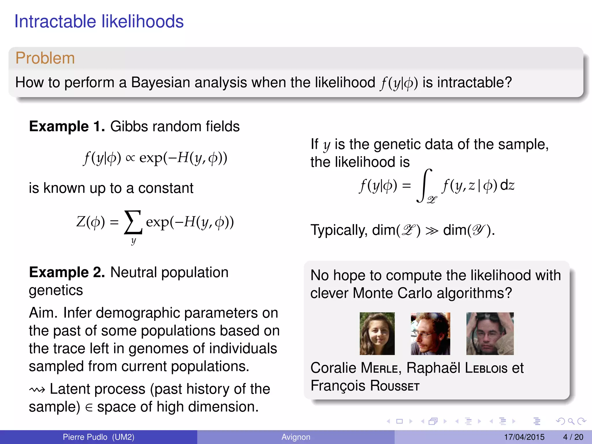
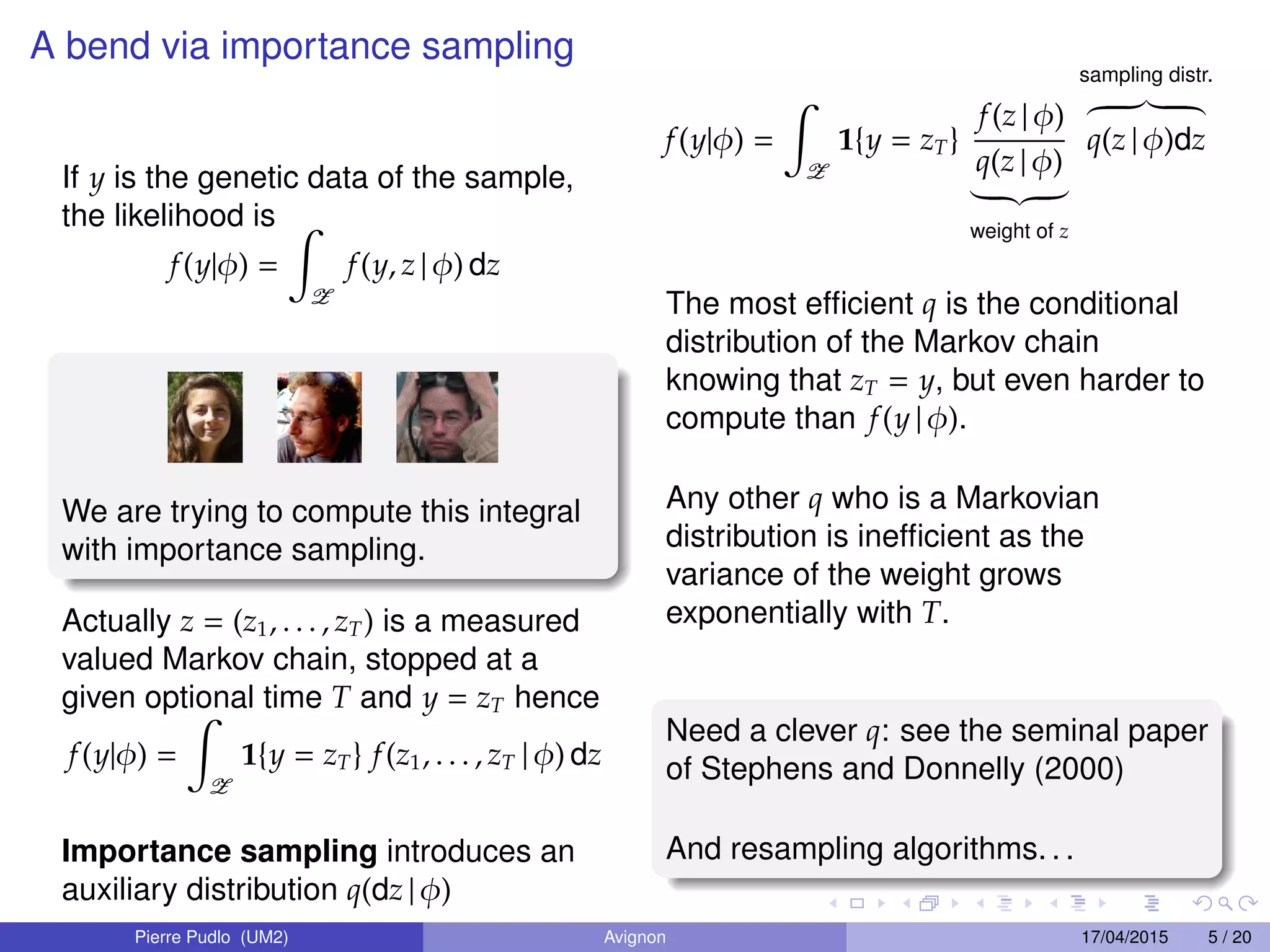
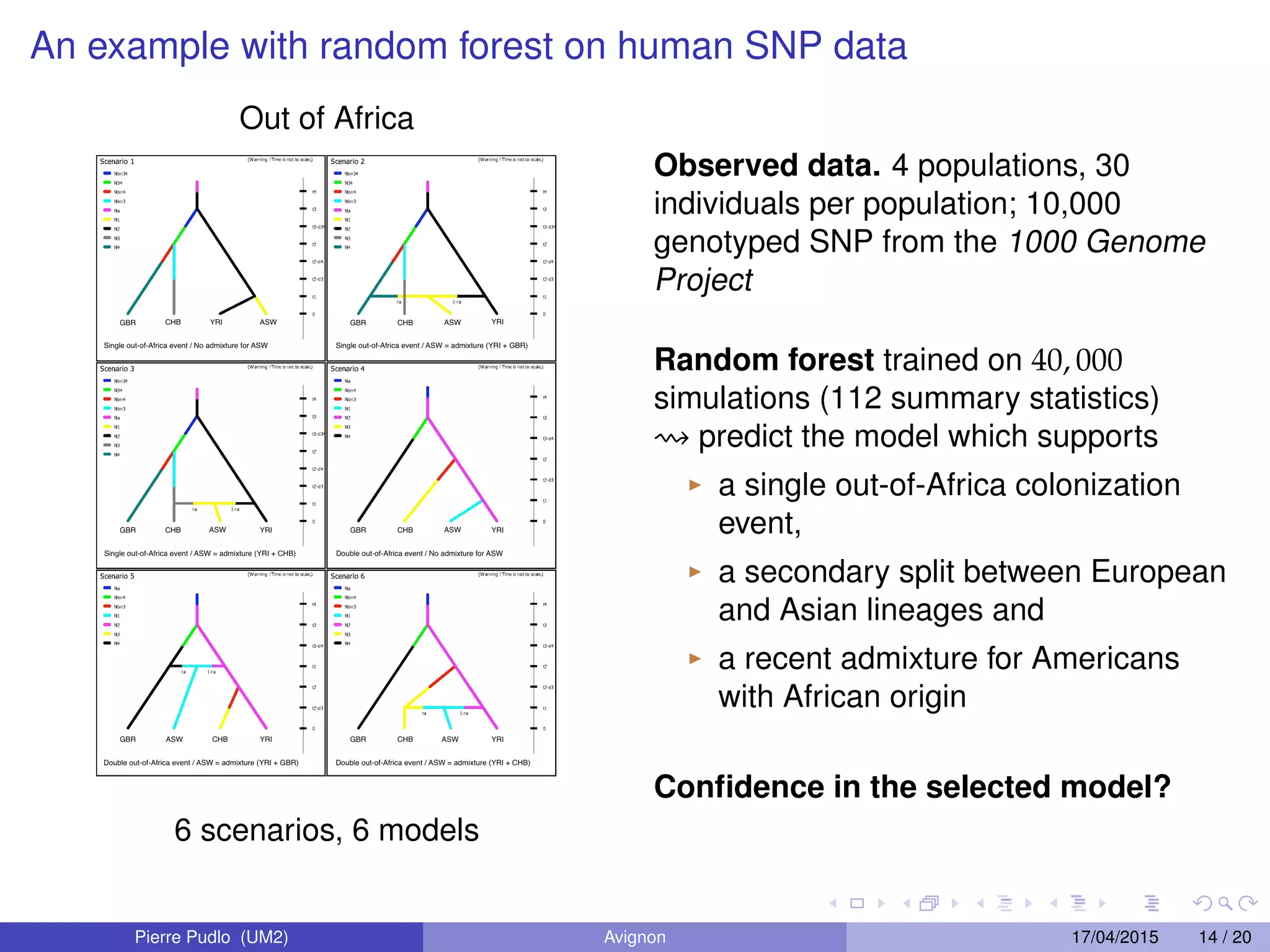
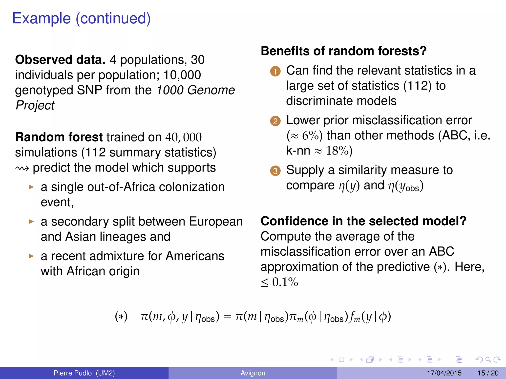
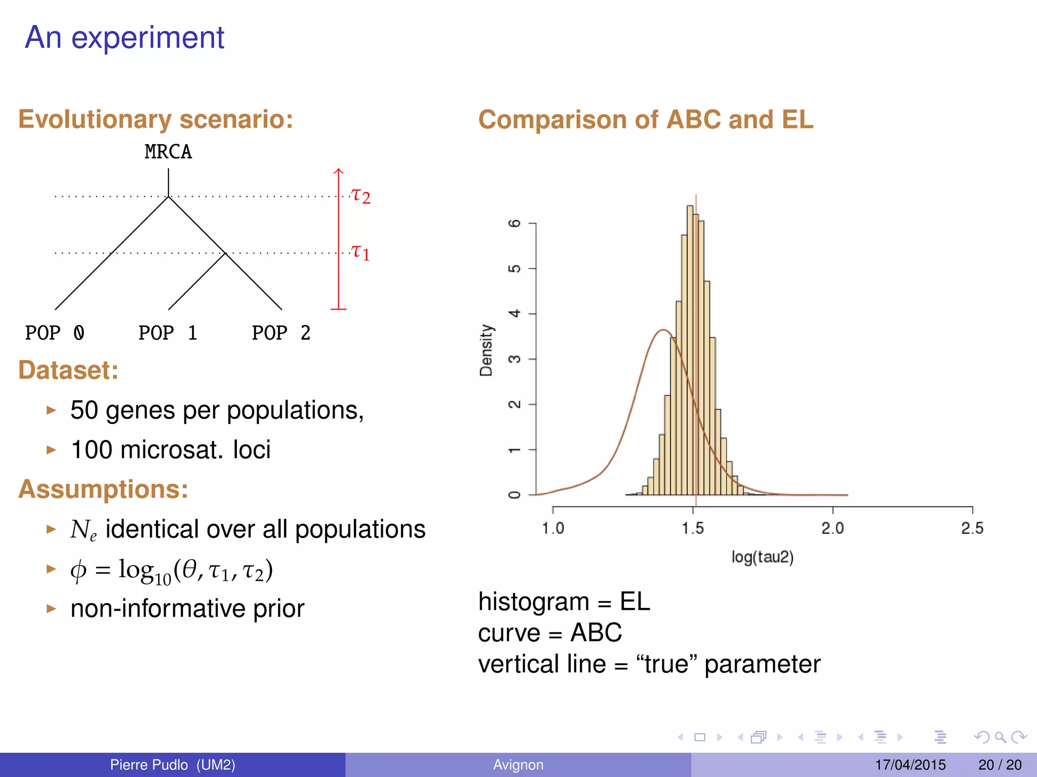

1. The document discusses likelihood-free computational statistics methods for Bayesian inference when the likelihood function is intractable. It covers approximate Bayesian computation (ABC), ABC model choice, and Bayesian computation using empirical likelihood. 2. ABC approximates the posterior distribution by simulating data under different parameter values and retaining simulations that best match the observed data. ABC model choice extends this to model selection problems. 3. Empirical likelihood provides an alternative to ABC by reconstructing a likelihood function from independent blocks of data, allowing faster Bayesian inference without loss of information from summary statistics.


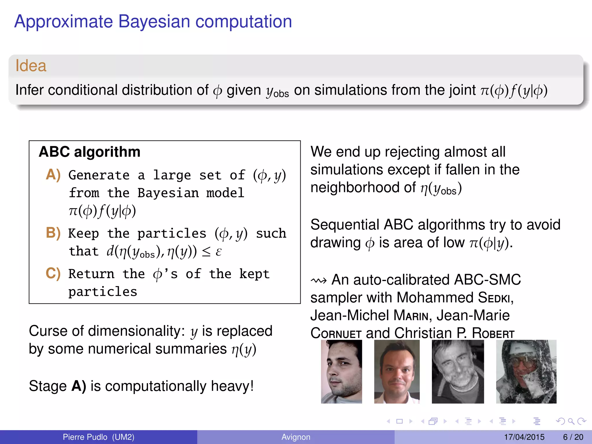
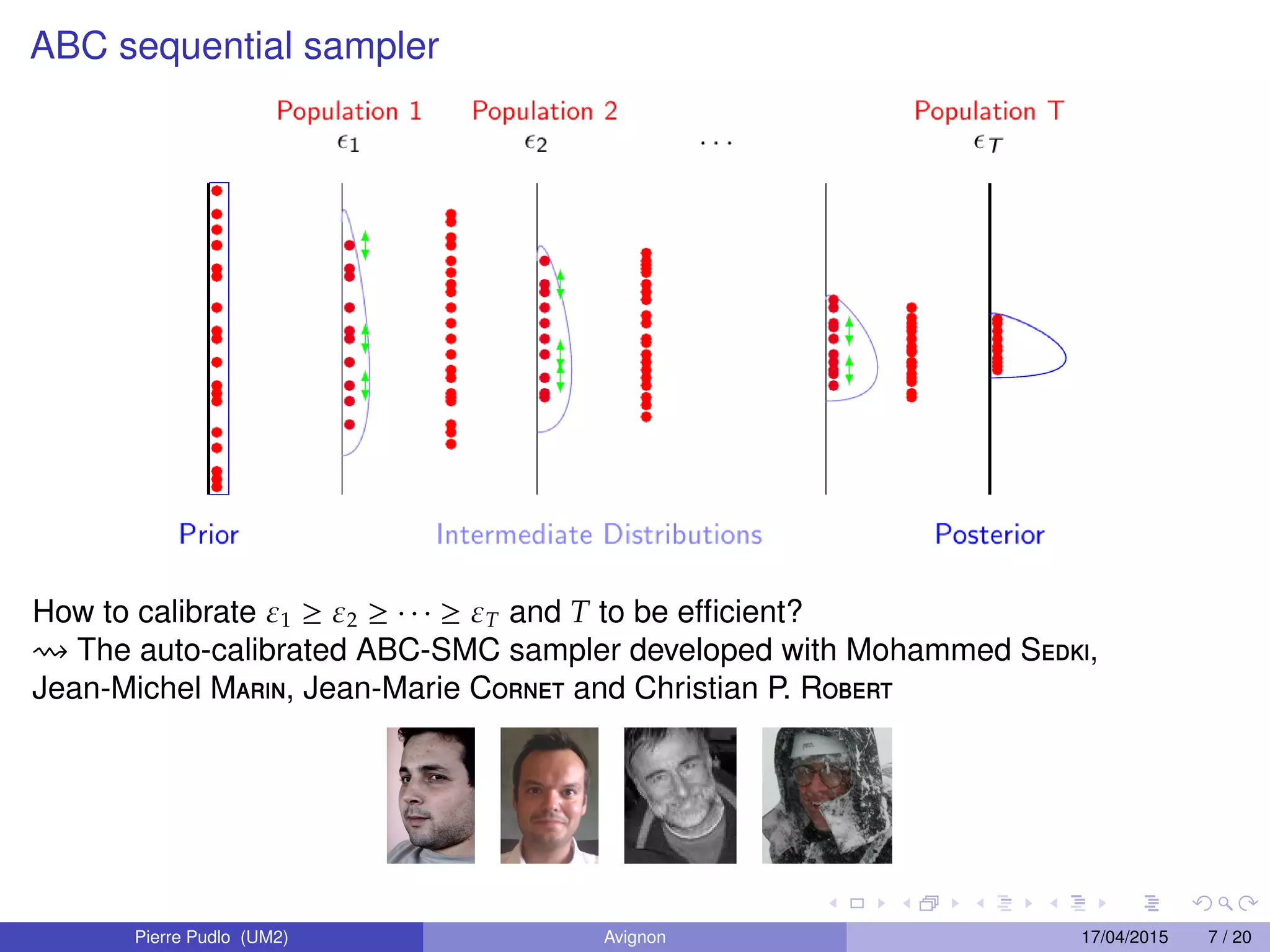
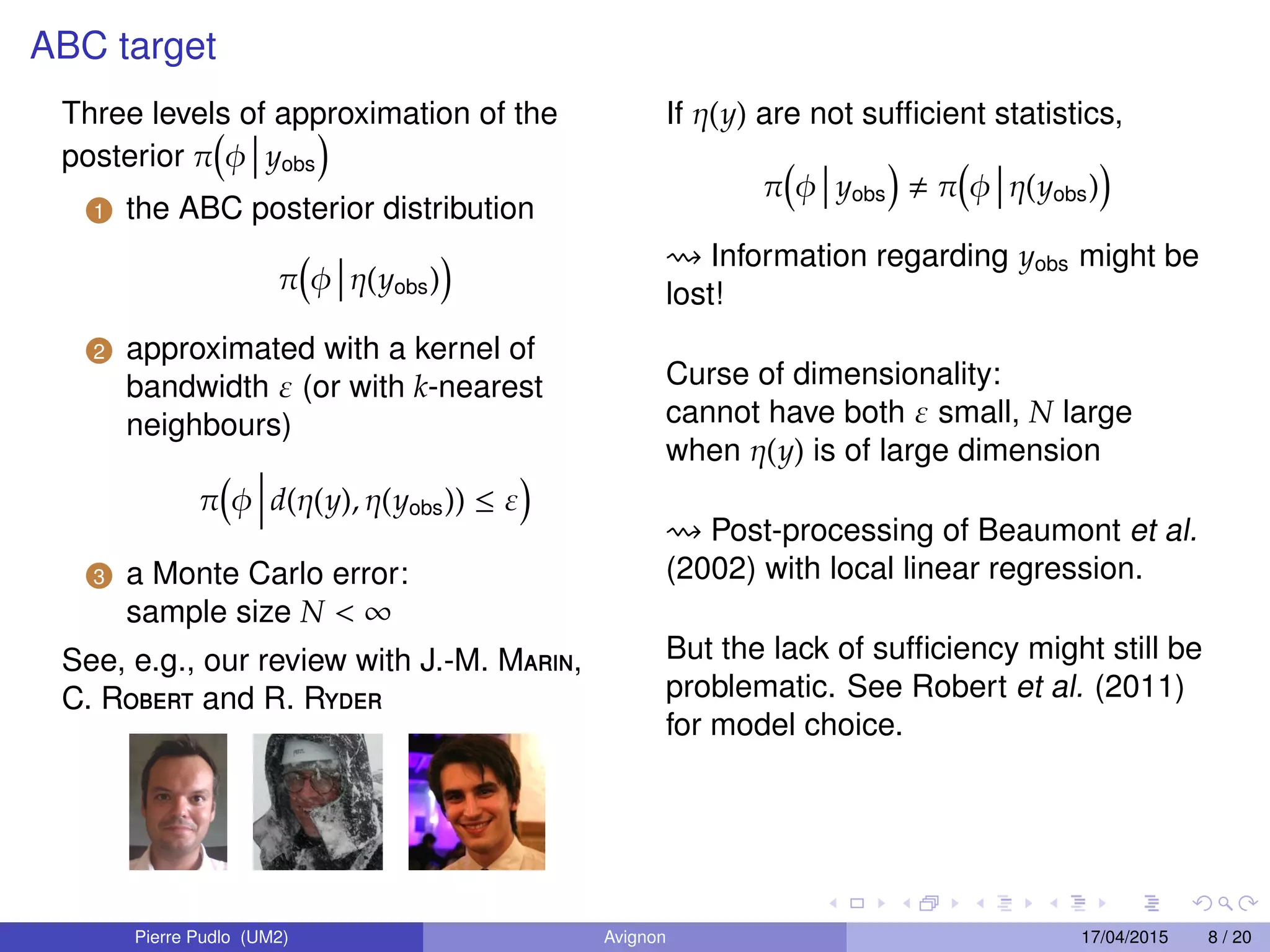
![Columbia workshop [ABC model choice]](https://cdn.slidesharecdn.com/ss_thumbnails/columbia-110924060002-phpapp01-thumbnail.jpg?width=640&height=640&fit=bounds)


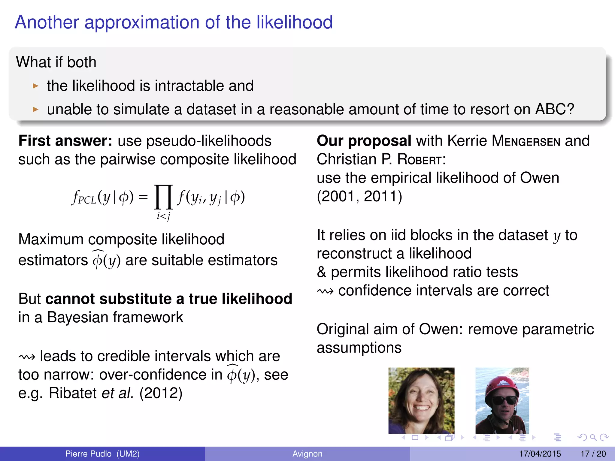
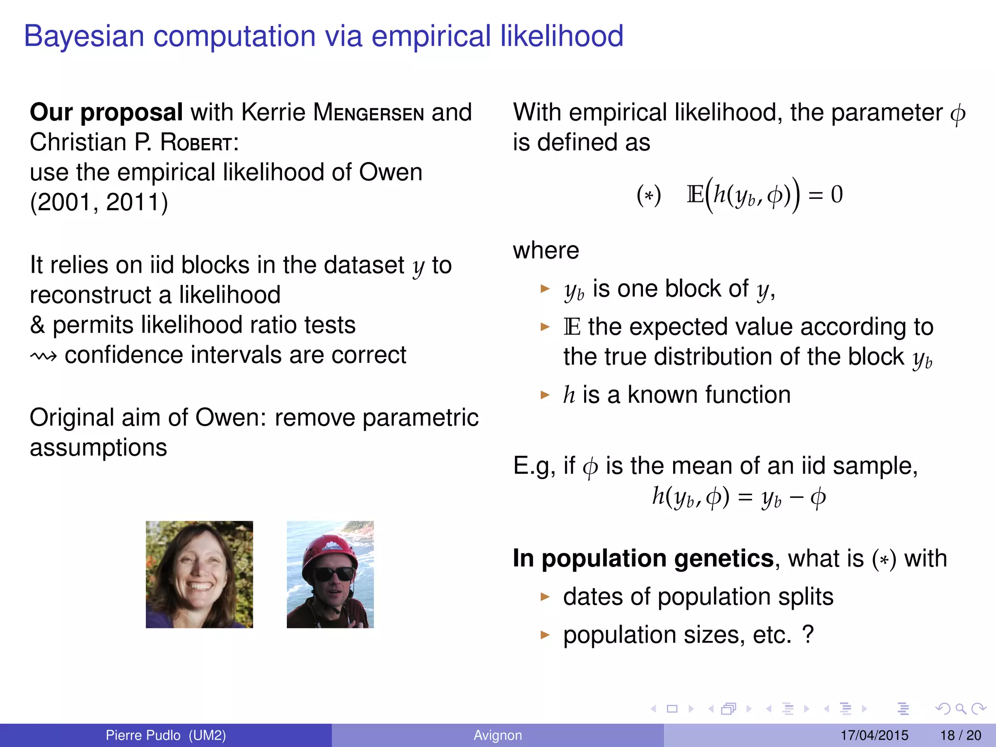
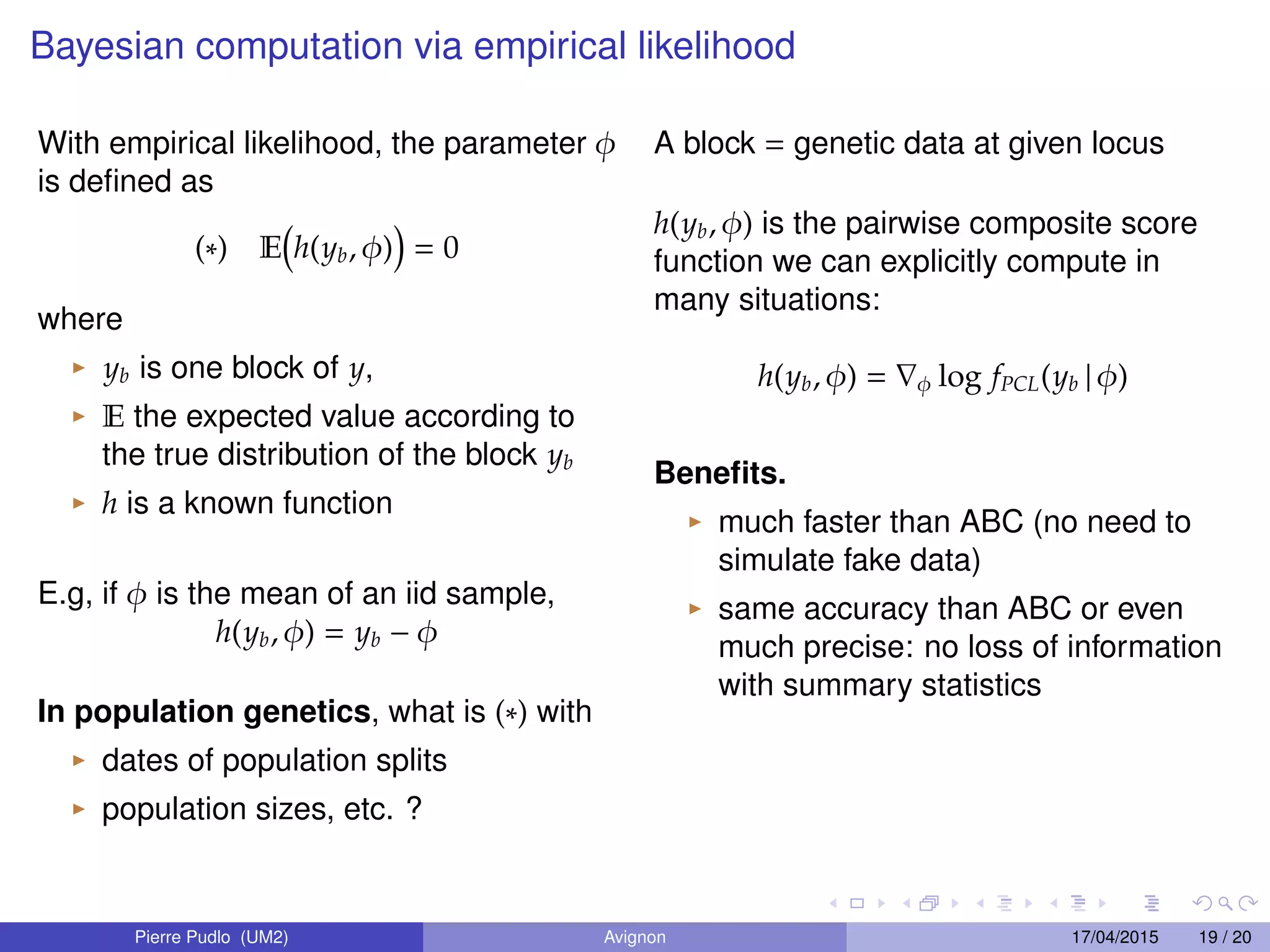
![[A]BCel : a presentation at ABC in Roma](https://cdn.slidesharecdn.com/ss_thumbnails/abcel-130530042650-phpapp02-thumbnail.jpg?width=640&height=640&fit=bounds)


