Download as PDF, PPTX
![ABC Methods for Bayesian Model Choice
Approximate Bayesian computation
Regular Bayesian computation issues
When faced with a non-standard posterior distribution
π(θ|y) ∝ π(θ)L(θ|y)
the standard solution is to use simulation (Monte Carlo) to
produce a sample
θ1 , . . . , θ T
from π(θ|y) (or approximately by Markov chain Monte Carlo
methods)
[Robert & Casella, 2004]](https://image.slidesharecdn.com/edinburgh-110905100913-phpapp02/75/Edinburgh-Bayes-250-3-2048.jpg)


![ABC Methods for Bayesian Model Choice
Approximate Bayesian computation
The ABC method
Bayesian setting: target is π(θ)f (x|θ)
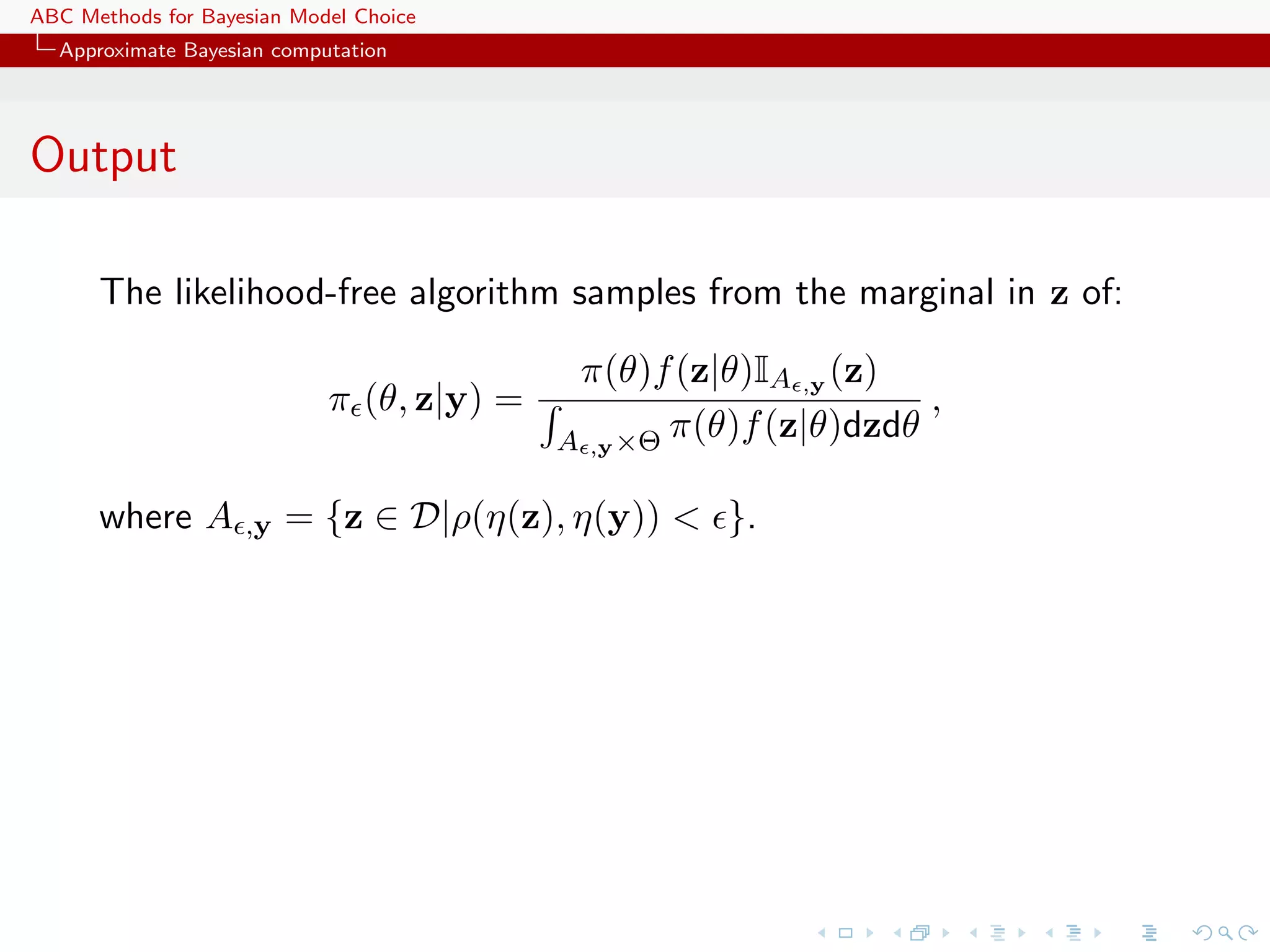
When likelihood f (x|θ) not in closed form, likelihood-free rejection
technique:
ABC algorithm
For an observation y ∼ f (y|θ), under the prior π(θ), keep jointly
simulating
θ ∼ π(θ) , z ∼ f (z|θ ) ,
until the auxiliary variable z is equal to the observed value, z = y.
[Tavar´ et al., 1997]
e](https://image.slidesharecdn.com/edinburgh-110905100913-phpapp02/75/Edinburgh-Bayes-250-8-2048.jpg)


![ABC Methods for Bayesian Model Choice
ABC for model choice
Generic ABC for model choice
Algorithm 2 Likelihood-free model choice sampler (ABC-MC)
for t = 1 to T do
repeat
Generate m from the prior π(M = m)
Generate θ m from the prior πm (θ m )
Generate z from the model fm (z|θ m )
until ρ{η(z), η(y)} <
Set m(t) = m and θ (t) = θ m
end for
[Toni, Welch, Strelkowa, Ipsen & Stumpf, 2009]](https://image.slidesharecdn.com/edinburgh-110905100913-phpapp02/75/Edinburgh-Bayes-250-22-2048.jpg)

![ABC Methods for Bayesian Model Choice
ABC for model choice
ABC estimates
Posterior probability π(M = m|y) approximated by the frequency
of acceptances from model m
T
1
Im(t) =m .
T
t=1
Early issues with implementation:
then needs to become part of the model
Varying statistics incompatible with Bayesian model choice
proper
ρ then part of the model
Extension to a weighted polychotomous logistic regression estimate
of π(M = m|y), with non-parametric kernel weights
[Cornuet et al., DIYABC, 2009]](https://image.slidesharecdn.com/edinburgh-110905100913-phpapp02/75/Edinburgh-Bayes-250-24-2048.jpg)
![ABC Methods for Bayesian Model Choice
ABC for model choice
The great ABC controversy
On-going controvery in phylogeographic genetics about the validity
of using ABC for testing
Replies: Fagundes et al., 2008,
Against: Templeton, 2008, Beaumont et al., 2010, Berger et
2009, 2010a, 2010b, 2010c, &tc al., 2010, Csill`ry et al., 2010
e
argues that nested hypotheses point out that the criticisms are
cannot have higher probabilities addressed at [Bayesian]
than nesting hypotheses (!) model-based inference and have
nothing to do with ABC...](https://image.slidesharecdn.com/edinburgh-110905100913-phpapp02/75/Edinburgh-Bayes-250-26-2048.jpg)

![ABC Methods for Bayesian Model Choice
Gibbs random fields
Potts model
Potts model
c∈C Vc (y) is of the form
Vc (y) = θS(y) = θ δyl =yi
c∈C l∼i
where l∼i denotes a neighbourhood structure
In most realistic settings, summation
Zθ = exp{θ T S(x)}
x∈X
involves too many terms to be manageable and numerical
approximations cannot always be trusted
[Cucala et al., 2009]](https://image.slidesharecdn.com/edinburgh-110905100913-phpapp02/75/Edinburgh-Bayes-250-28-2048.jpg)


![ABC Methods for Bayesian Model Choice
Generic ABC model choice
Back to sufficiency
‘Sufficient statistics for individual models are unlikely to
be very informative for the model probability. This is
already well known and understood by the ABC-user
community.’
[Scott Sisson, Jan. 31, 2011, ’Og]](https://image.slidesharecdn.com/edinburgh-110905100913-phpapp02/75/Edinburgh-Bayes-250-37-2048.jpg)
![ABC Methods for Bayesian Model Choice
Generic ABC model choice
Back to sufficiency
‘Sufficient statistics for individual models are unlikely to
be very informative for the model probability. This is
already well known and understood by the ABC-user
community.’
[Scott Sisson, Jan. 31, 2011, ’Og]
If η1 (x) sufficient statistic for model m = 1 and parameter θ1 and
η2 (x) sufficient statistic for model m = 2 and parameter θ2 ,
(η1 (x), η2 (x)) is not always sufficient for (m, θm )](https://image.slidesharecdn.com/edinburgh-110905100913-phpapp02/75/Edinburgh-Bayes-250-38-2048.jpg)
![ABC Methods for Bayesian Model Choice
Generic ABC model choice
Back to sufficiency
‘Sufficient statistics for individual models are unlikely to
be very informative for the model probability. This is
already well known and understood by the ABC-user
community.’
[Scott Sisson, Jan. 31, 2011, ’Og]
If η1 (x) sufficient statistic for model m = 1 and parameter θ1 and
η2 (x) sufficient statistic for model m = 2 and parameter θ2 ,
(η1 (x), η2 (x)) is not always sufficient for (m, θm )
c Potential loss of information at the testing level](https://image.slidesharecdn.com/edinburgh-110905100913-phpapp02/75/Edinburgh-Bayes-250-39-2048.jpg)


![ABC Methods for Bayesian Model Choice
Generic ABC model choice
Limiting behaviour of B12 (under sufficiency)
If η(y) sufficient statistic in both models,
fi (y|θ i ) = gi (y)fiη (η(y)|θ i )
Thus
η
Θ1 π(θ 1 )g1 (y)f1 (η(y)|θ 1 ) dθ 1
B12 (y) = η
Θ2 π(θ 2 )g2 (y)f2 (η(y)|θ 2 ) dθ 2
η
g1 (y) π1 (θ 1 )f1 (η(y)|θ 1 ) dθ 1 g1 (y) η
= η = B (y) .
g2 (y) π2 (θ 2 )f2 (η(y)|θ 2 ) dθ 2 g2 (y) 12
[Didelot, Everitt, Johansen & Lawson, 2011]](https://image.slidesharecdn.com/edinburgh-110905100913-phpapp02/75/Edinburgh-Bayes-250-44-2048.jpg)
![ABC Methods for Bayesian Model Choice
Generic ABC model choice
Limiting behaviour of B12 (under sufficiency)
If η(y) sufficient statistic in both models,
fi (y|θ i ) = gi (y)fiη (η(y)|θ i )
Thus
η
Θ1 π(θ 1 )g1 (y)f1 (η(y)|θ 1 ) dθ 1
B12 (y) = η
Θ2 π(θ 2 )g2 (y)f2 (η(y)|θ 2 ) dθ 2
η
g1 (y) π1 (θ 1 )f1 (η(y)|θ 1 ) dθ 1 g1 (y) η
= η = B (y) .
g2 (y) π2 (θ 2 )f2 (η(y)|θ 2 ) dθ 2 g2 (y) 12
[Didelot, Everitt, Johansen & Lawson, 2011]
c No discrepancy only when cross-model sufficiency](https://image.slidesharecdn.com/edinburgh-110905100913-phpapp02/75/Edinburgh-Bayes-250-45-2048.jpg)


![ABC Methods for Bayesian Model Choice
Generic ABC model choice
Formal recovery
Creating an encompassing exponential family
T T
f (x|θ1 , θ2 , α1 , α2 ) ∝ exp{θ1 η1 (x) + θ1 η1 (x) + α1 t1 (x) + α2 t2 (x)}
leads to a sufficient statistic (η1 (x), η2 (x), t1 (x), t2 (x))
[Didelot, Everitt, Johansen & Lawson, 2011]](https://image.slidesharecdn.com/edinburgh-110905100913-phpapp02/75/Edinburgh-Bayes-250-48-2048.jpg)
![ABC Methods for Bayesian Model Choice
Generic ABC model choice
Formal recovery
Creating an encompassing exponential family
T T
f (x|θ1 , θ2 , α1 , α2 ) ∝ exp{θ1 η1 (x) + θ1 η1 (x) + α1 t1 (x) + α2 t2 (x)}
leads to a sufficient statistic (η1 (x), η2 (x), t1 (x), t2 (x))
[Didelot, Everitt, Johansen & Lawson, 2011]
In the Poisson/geometric case, if i xi ! is added to S, no
discrepancy](https://image.slidesharecdn.com/edinburgh-110905100913-phpapp02/75/Edinburgh-Bayes-250-49-2048.jpg)
![ABC Methods for Bayesian Model Choice
Generic ABC model choice
Formal recovery
Creating an encompassing exponential family
T T
f (x|θ1 , θ2 , α1 , α2 ) ∝ exp{θ1 η1 (x) + θ1 η1 (x) + α1 t1 (x) + α2 t2 (x)}
leads to a sufficient statistic (η1 (x), η2 (x), t1 (x), t2 (x))
[Didelot, Everitt, Johansen & Lawson, 2011]
Only applies in genuine sufficiency settings...
c Inability to evaluate loss brought by summary statistics](https://image.slidesharecdn.com/edinburgh-110905100913-phpapp02/75/Edinburgh-Bayes-250-50-2048.jpg)
![ABC Methods for Bayesian Model Choice
Generic ABC model choice
The Pitman–Koopman lemma
Efficient sufficiency is not such a common occurrence:
Lemma
A necessary and sufficient condition for the existence of a sufficient
statistic with fixed dimension whatever the sample size is that the
sampling distribution belongs to an exponential family.
[Pitman, 1933; Koopman, 1933]](https://image.slidesharecdn.com/edinburgh-110905100913-phpapp02/75/Edinburgh-Bayes-250-51-2048.jpg)
![ABC Methods for Bayesian Model Choice
Generic ABC model choice
The Pitman–Koopman lemma
Efficient sufficiency is not such a common occurrence:
Lemma
A necessary and sufficient condition for the existence of a sufficient
statistic with fixed dimension whatever the sample size is that the
sampling distribution belongs to an exponential family.
[Pitman, 1933; Koopman, 1933]
Provision of fixed support (consider U(0, θ) counterexample)](https://image.slidesharecdn.com/edinburgh-110905100913-phpapp02/75/Edinburgh-Bayes-250-52-2048.jpg)
![ABC Methods for Bayesian Model Choice
Generic ABC model choice
Meaning of the ABC-Bayes factor
‘This is also why focus on model discrimination typically
(...) proceeds by (...) accepting that the Bayes Factor
that one obtains is only derived from the summary
statistics and may in no way correspond to that of the
full model.’
[Scott Sisson, Jan. 31, 2011, ’Og]](https://image.slidesharecdn.com/edinburgh-110905100913-phpapp02/75/Edinburgh-Bayes-250-53-2048.jpg)
![ABC Methods for Bayesian Model Choice
Generic ABC model choice
Meaning of the ABC-Bayes factor
‘This is also why focus on model discrimination typically
(...) proceeds by (...) accepting that the Bayes Factor
that one obtains is only derived from the summary
statistics and may in no way correspond to that of the
full model.’
[Scott Sisson, Jan. 31, 2011, ’Og]
In the Poisson/geometric case, if E[yi ] = θ0 > 0,
η (θ0 + 1)2 −θ0
lim B12 (y) = e
n→∞ θ0](https://image.slidesharecdn.com/edinburgh-110905100913-phpapp02/75/Edinburgh-Bayes-250-54-2048.jpg)
![ABC Methods for Bayesian Model Choice
Generic ABC model choice
MA example
0.7
0.6
0.6
0.6
0.6
0.5
0.5
0.5
0.5
0.4
0.4
0.4
0.4
0.3
0.3
0.3
0.3
0.2
0.2
0.2
0.2
0.1
0.1
0.1
0.1
0.0
0.0
0.0
0.0
1 2 1 2 1 2 1 2
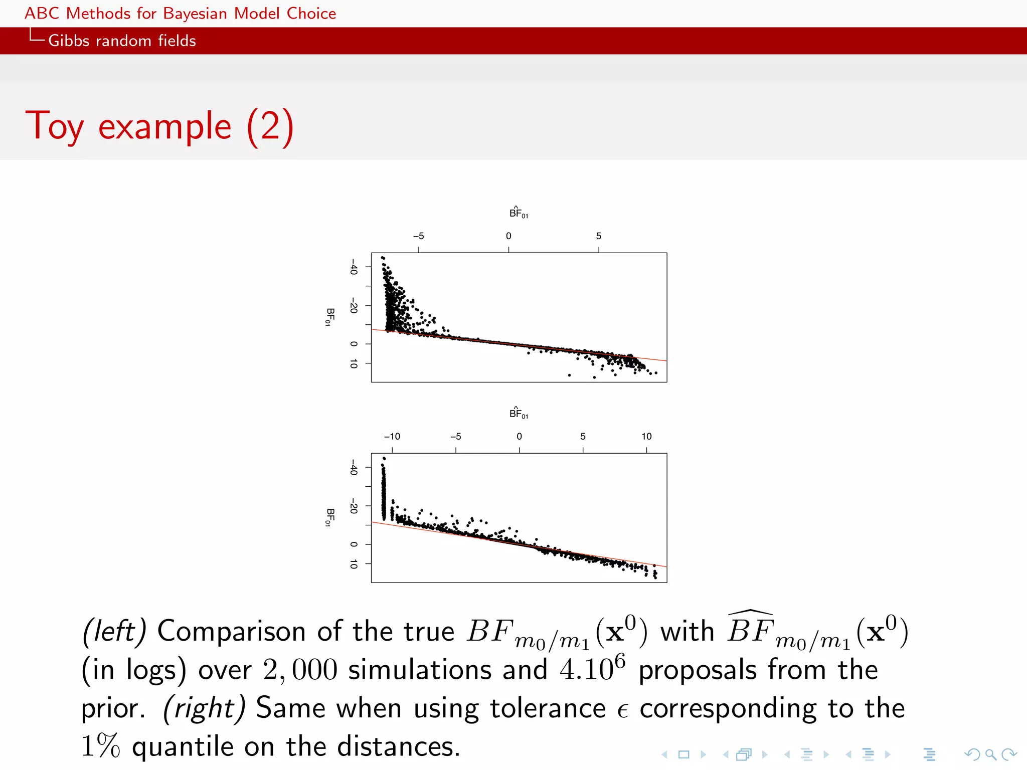
Evolution [against ] of ABC Bayes factor, in terms of frequencies of
visits to models MA(1) (left) and MA(2) (right) when equal to
10, 1, .1, .01% quantiles on insufficient autocovariance distances. Sample
of 50 points from a MA(2) with θ1 = 0.6, θ2 = 0.2. True Bayes factor
equal to 17.71.](https://image.slidesharecdn.com/edinburgh-110905100913-phpapp02/75/Edinburgh-Bayes-250-55-2048.jpg)
![ABC Methods for Bayesian Model Choice
Generic ABC model choice
MA example
0.8
0.6
0.6
0.6
0.6
0.4
0.4
0.4
0.4
0.2
0.2
0.2
0.2
0.0
0.0
0.0
0.0
1 2 1 2 1 2 1 2
Evolution [against ] of ABC Bayes factor, in terms of frequencies of
visits to models MA(1) (left) and MA(2) (right) when equal to
10, 1, .1, .01% quantiles on insufficient autocovariance distances. Sample
of 50 points from a MA(1) model with θ1 = 0.6. True Bayes factor B21
equal to .004.](https://image.slidesharecdn.com/edinburgh-110905100913-phpapp02/75/Edinburgh-Bayes-250-56-2048.jpg)
![ABC Methods for Bayesian Model Choice
Generic ABC model choice
Further comments
‘There should be the possibility that for the same model,
but different (non-minimal) [summary] statistics (so
∗
different η’s: η1 and η1 ) the ratio of evidences may no
longer be equal to one.’
[Michael Stumpf, Jan. 28, 2011, ’Og]
Using different summary statistics [on different models] may
indicate the loss of information brought by each set but agreement
does not lead to trustworthy approximations.](https://image.slidesharecdn.com/edinburgh-110905100913-phpapp02/75/Edinburgh-Bayes-250-57-2048.jpg)
![ABC Methods for Bayesian Model Choice
Generic ABC model choice
A population genetics evaluation
Population genetics example with
3 populations
2 scenari
15 individuals
5 loci
single mutation parameter
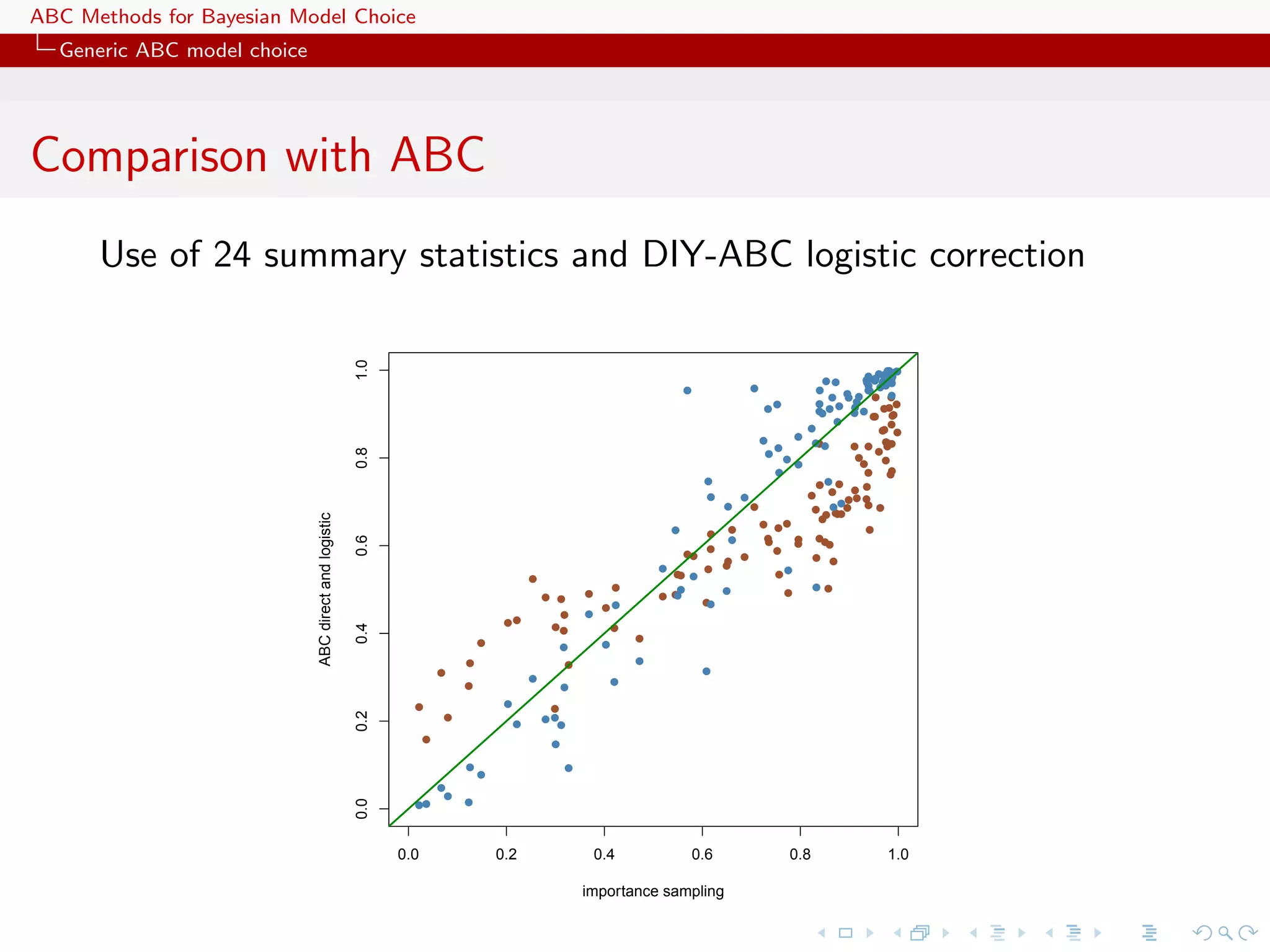
24 summary statistics
2 million ABC proposal
importance [tree] sampling alternative](https://image.slidesharecdn.com/edinburgh-110905100913-phpapp02/75/Edinburgh-Bayes-250-59-2048.jpg)


![ABC Methods for Bayesian Model Choice
Generic ABC model choice
A second population genetics experiment
three populations, two divergent 100 gen. ago
two scenarios [third pop. recent admixture between first two
pop. / diverging from pop. 1 5 gen. ago]
In scenario 1, admixture rate 0.7 from pop. 1
100 datasets with 100 diploid individuals per population, 50
independent microsatellite loci.
Effective population size of 1000 and mutation rates of
0.0005.
6 parameters: admixture rate (U [0.1, 0.9]), three effective
population sizes (U [200, 2000]), the time of admixture/second
divergence (U [1, 10]) and time of first divergence (U [50, 500]).](https://image.slidesharecdn.com/edinburgh-110905100913-phpapp02/75/Edinburgh-Bayes-250-65-2048.jpg)
![ABC Methods for Bayesian Model Choice
Generic ABC model choice
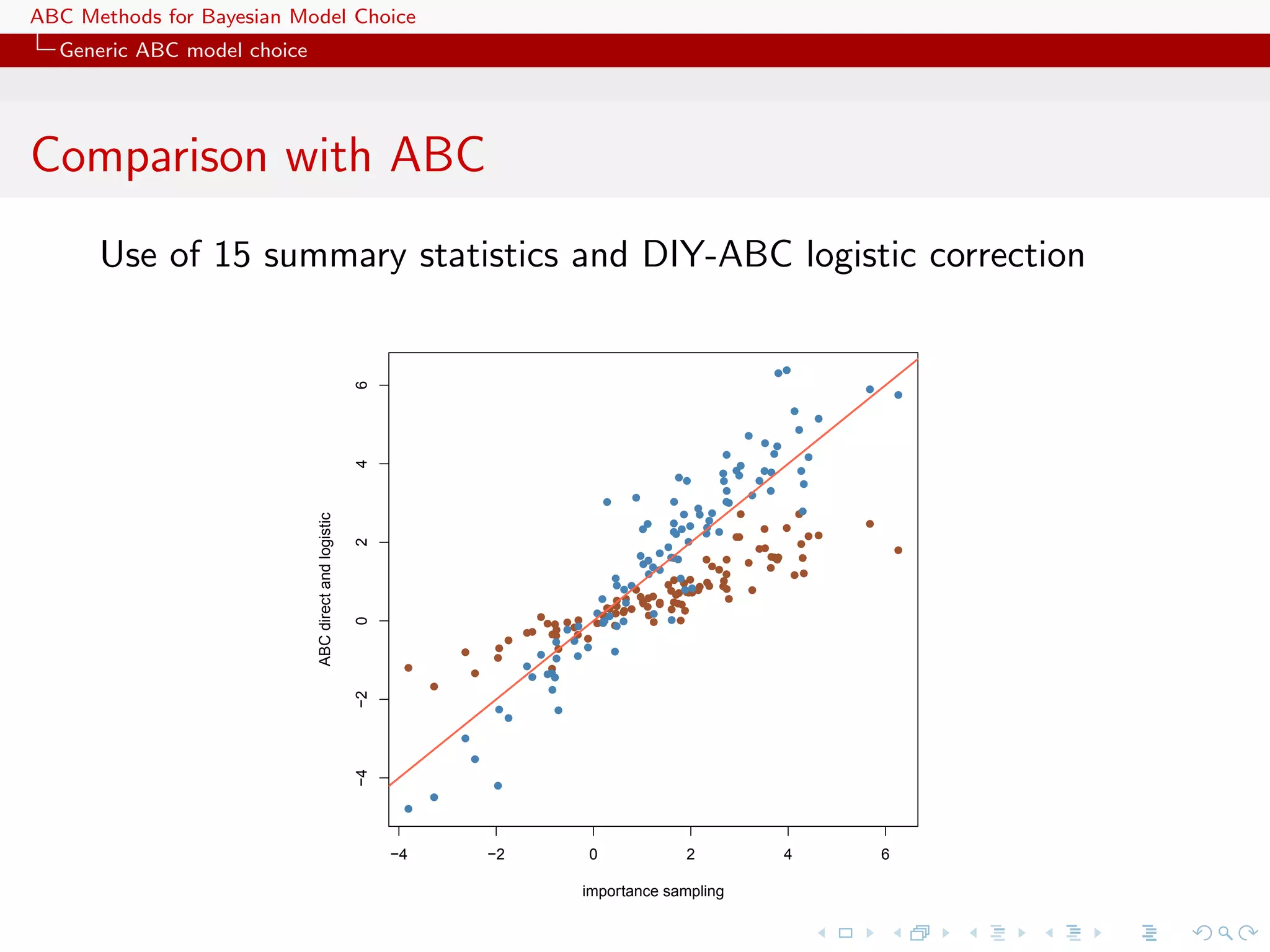
Results
IS algorithm performed with 100 coalescent trees per particle and
50,000 particles [12 calendar days using 376 processors]
Using ten times as many loci and seven times as many individuals
degrades the confidence in the importance sampling approximation
because of an increased variability in the likelihood. 1.0
q qq q qq q q qqqq
qq
q
q qq
q
q
q q qq
qq
q
q
qq
q
q q
q
q
0.8
q
Importance Sampling estimates of
q
P(M=1|y) with 1,000 particles
q q
0.6
0.4
0.2
0.0
0.0 0.2 0.4 0.6 0.8 1.0
Importance Sampling estimates of](https://image.slidesharecdn.com/edinburgh-110905100913-phpapp02/75/Edinburgh-Bayes-250-66-2048.jpg)

![ABC Methods for Bayesian Model Choice
Generic ABC model choice
The only safe cases???
Besides specific models like Gibbs random fields,
using distances over the data itself escapes the discrepancy...
[Toni & Stumpf, 2010;Sousa et al., 2009]](https://image.slidesharecdn.com/edinburgh-110905100913-phpapp02/75/Edinburgh-Bayes-250-68-2048.jpg)
![ABC Methods for Bayesian Model Choice
Generic ABC model choice
The only safe cases???
Besides specific models like Gibbs random fields,
using distances over the data itself escapes the discrepancy...
[Toni & Stumpf, 2010;Sousa et al., 2009]
...and so does the use of more informal model fitting measures
[Ratmann, Andrieu, Richardson and Wiujf, 2009]](https://image.slidesharecdn.com/edinburgh-110905100913-phpapp02/75/Edinburgh-Bayes-250-69-2048.jpg)

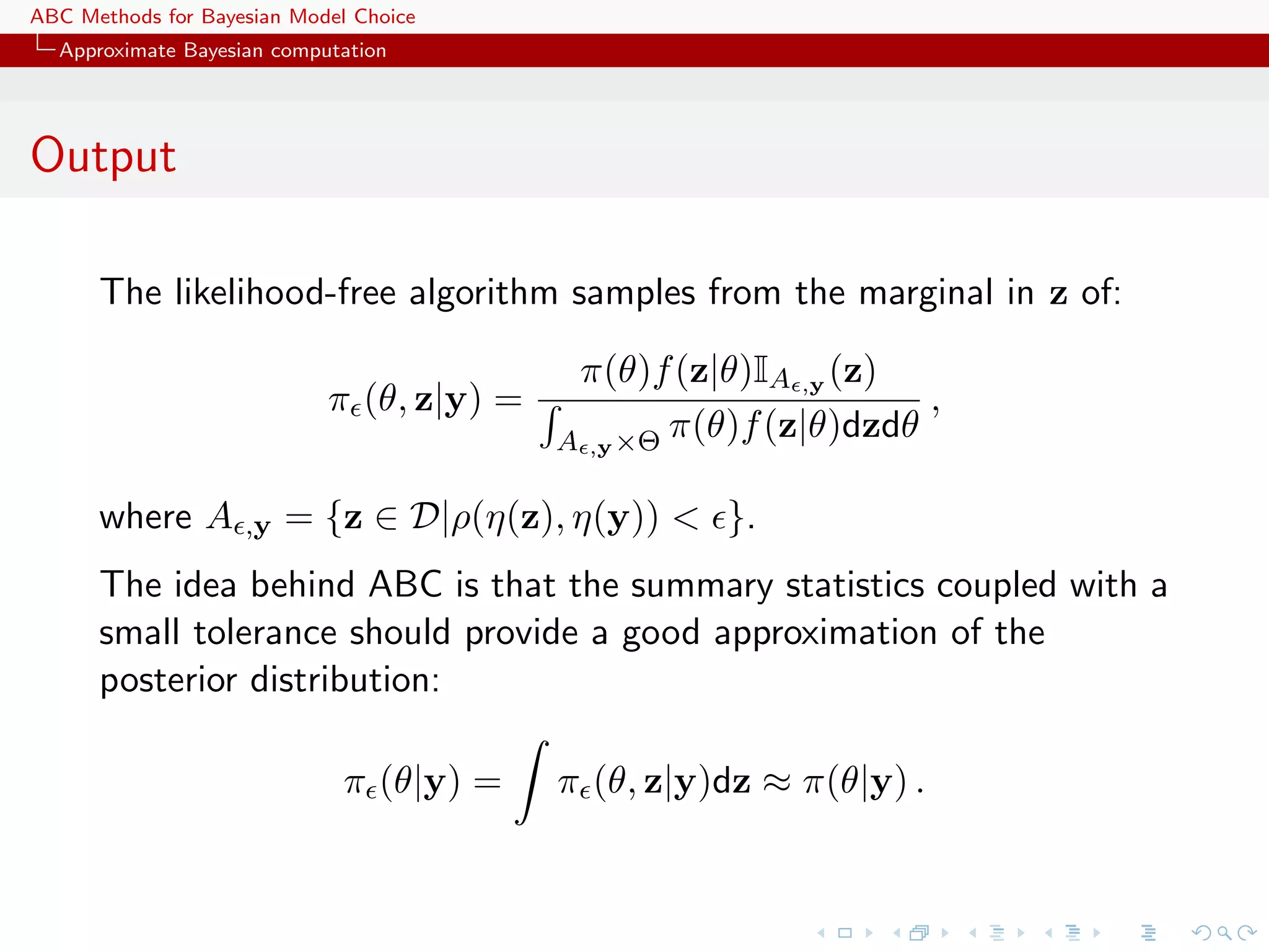
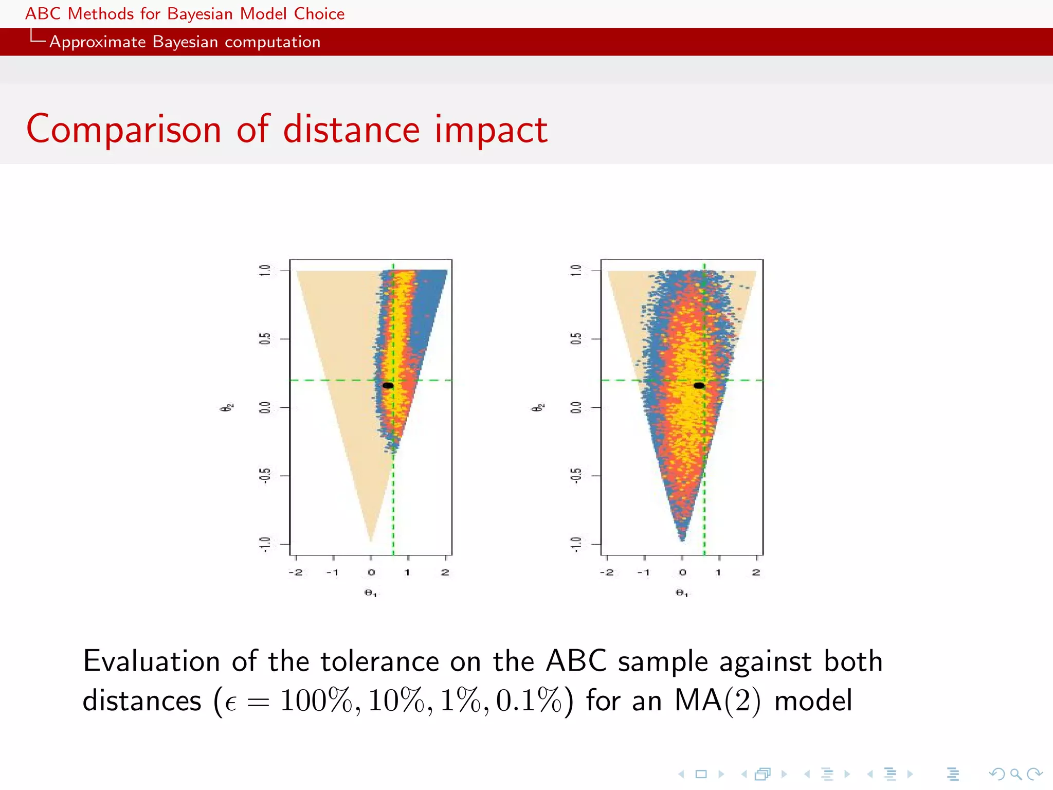
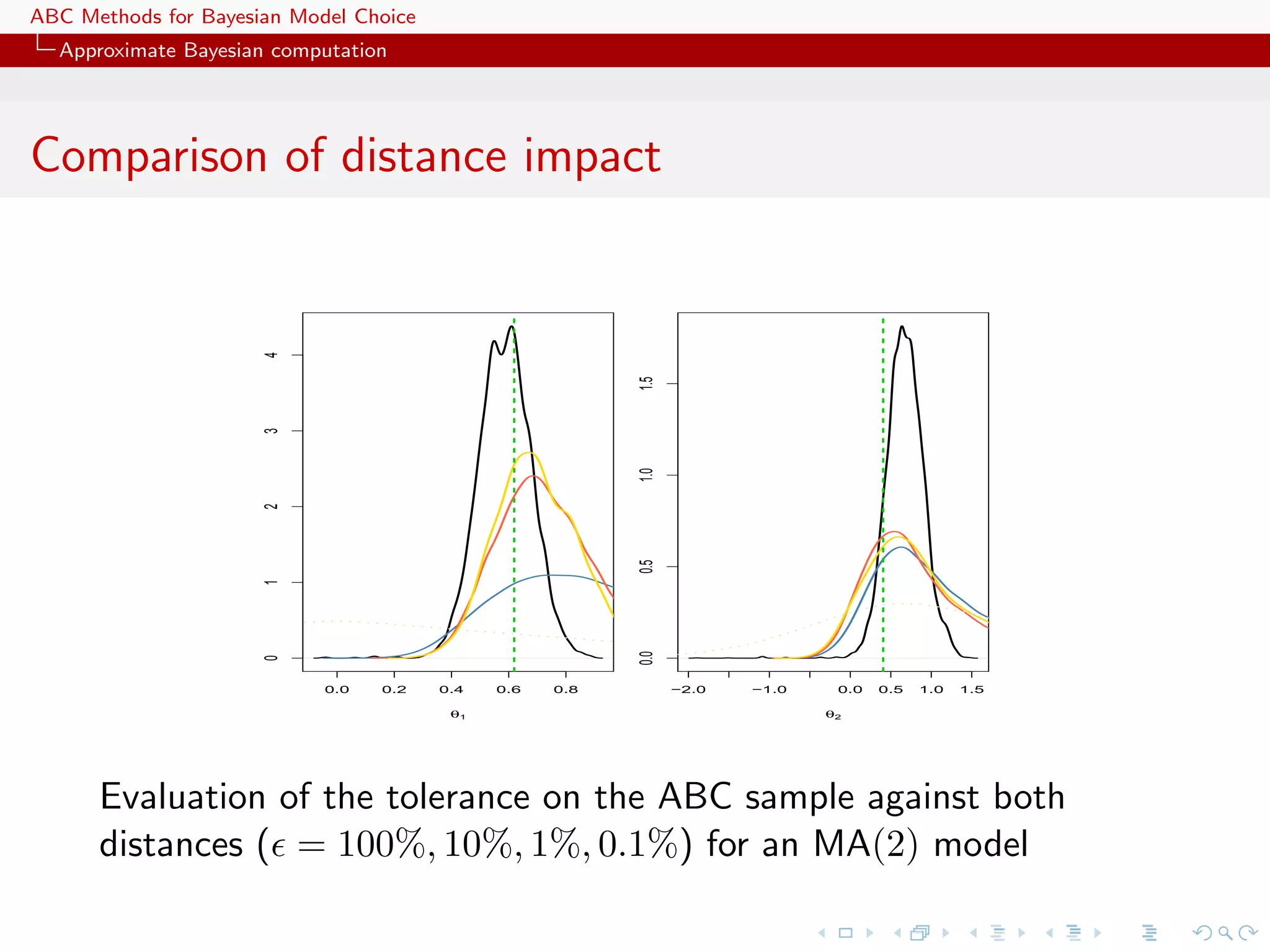
The document discusses approximate Bayesian computation (ABC) methods for Bayesian model choice when likelihoods are intractable. It introduces ABC, which approximates posteriors by simulating data under different parameter values and accepting simulations that are close to the observed data according to a distance measure. It then discusses applying ABC to model choice by simulating parameters and data from different candidate models. The document provides an example of using ABC for an MA time series model and compares distance measures. It also outlines a generic ABC algorithm for Bayesian model choice.
![Columbia workshop [ABC model choice]](https://cdn.slidesharecdn.com/ss_thumbnails/columbia-110924060002-phpapp01-thumbnail.jpg?width=640&height=640&fit=bounds)


![Inference in generative models using the Wasserstein distance [[INI]](https://cdn.slidesharecdn.com/ss_thumbnails/inewton-170706120746-thumbnail.jpg?width=640&height=640&fit=bounds)