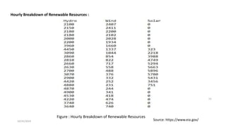
Download to read offline


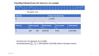
![Objectives:
• Network Optimization(Opening unnecessary line section)
and radial network reduces the line loss and removes the
circulating current throughout the network.
• Matching or opening available energy sources according to
load demand reduces the generation cost, operating cost
and saves the extra power.
• Most of the demand satisfy by the Hydro-electric power if
demand not exceed. [Ref]
[Ref]: 1 megawatt-hour of electricity costs $90.3 in 2011 to generate using hydropower and $144.30
to generate using solar collectors, according to the U.S. Energy Information](https://image.slidesharecdn.com/ga-191025204615/85/A-Genetic-Algorithm-Approach-to-Optimize-Dispatching-for-A-Micro-grid-Energy-System-with-Renewable-Energy-Sources-2-320.jpg)
![10/25/2019 3
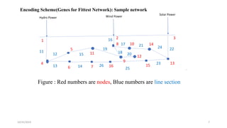
Algorithm:
Step 1: Initialize population of size N
for each population Initialize chromosome of size M=24 [24 for hours from 1AM to 12 AM]
for every chromosome initialize two types of genes: [ 2 types for 2 objectives]
Initialize genes for sources of size 3(3 bit) [ for optimizing energy sources]
Initialize genes for fittest network() of size 14 [ for network optimization]
for every chromosome calculate chromosome fitness based on fittest from both genes
Step 2:
For G number of generation
Evolve N population through Crossover & Mutation
Step 3: Output the fittest chromosome
Procedure of fittest network():
Initialize population of power network of size P of Graph G=(V,E)
Initialize chromosome of size Q [ Here 14] by check()
For R number of generation evolve population through crossover and mutation
Output: Fittest network after r generation
end
Procedure of check():
1 Generate Q number of genes of size 1 ( Random number from 1 to 16) by randomly deleting two edges and
checking Strong Connectivity through remaining edges. [Applied DFS to check strongly connectivity]
If not Strongly connected, repeat 1
Otherwise output the network.
end](https://image.slidesharecdn.com/ga-191025204615/85/A-Genetic-Algorithm-Approach-to-Optimize-Dispatching-for-A-Micro-grid-Energy-System-with-Renewable-Energy-Sources-3-320.jpg)
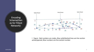
![10/25/2019 10
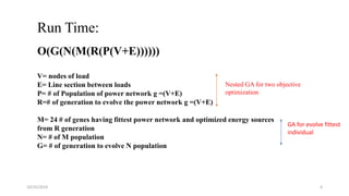
Fitness functions:
𝑝𝑒𝑛𝑎𝑙𝑖𝑧𝑒𝑑 𝑓𝑢𝑛𝑐𝑡𝑖𝑜𝑛, 𝑓𝐷 =
1, 𝑖𝑓𝐷𝑡 < 𝑗=1
𝑛
𝑃 𝑇𝑗
0, 𝑜𝑡ℎ𝑒𝑟𝑤𝑖𝑠𝑒
If Hydro power 𝑃 𝑇1 > 𝐷𝑖 and 𝑃 𝑇2 = 0 and 𝑃 𝑇3 = 0 [To use Hydro-electric power most ]
𝑓𝐻 =0.001 [Award]
If Hydro power & Wind power 𝑃 𝑇1 + 𝑃 𝑇2 > 𝐷𝑖 and 𝑃 𝑇3 = 0 & Hydro power 𝑃 𝑇1 < 𝐷𝑖
𝑓𝐻𝑊 =0.001 [Award]
𝑖=1
𝑅
min 𝑓𝐿 ; R is the number of generation occurred for network reconfiguration
𝐿𝑜𝑠𝑠 𝑓𝑢𝑛𝑐𝑡𝑖𝑜𝑛, 𝑓𝐿 = 𝑃𝐿𝑜𝑠𝑠 = 𝑖∈𝑁𝑖 𝐼𝑗
2
𝑅𝑖
where 𝐼𝑗 =
𝑃 𝑗
𝑉
=
𝑃 𝑗
220𝑘𝑉
, 𝑗 = 1,2 𝑎𝑛𝑑 3 and 𝑁𝑖= number of nodes
𝑉min < 𝑉𝑗 < 𝑉m𝑎𝑥
Individual gene fitness 𝑓𝑖 = 𝑓𝐷 * 𝑓𝐻 * 𝑓𝐻𝑊 * 𝑓𝐿
Total chromosome fitness = 𝑖=1
24
𝐹𝑖](https://image.slidesharecdn.com/ga-191025204615/85/A-Genetic-Algorithm-Approach-to-Optimize-Dispatching-for-A-Micro-grid-Energy-System-with-Renewable-Energy-Sources-10-320.jpg)


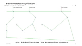
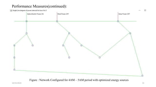

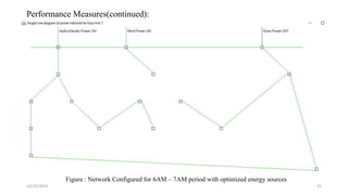
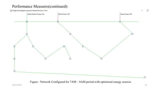
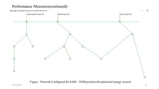
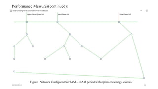
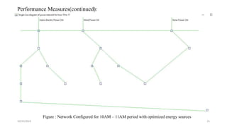
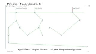
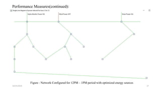
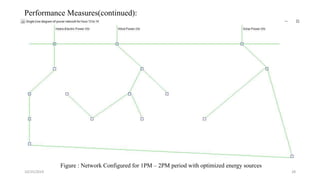
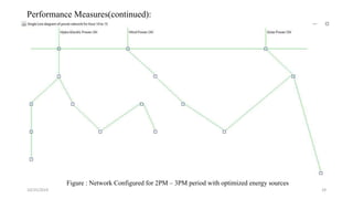
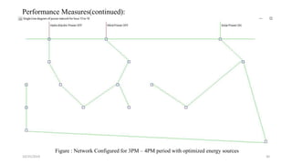
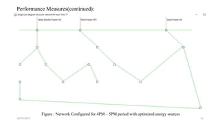
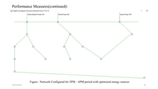
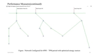
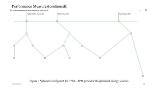
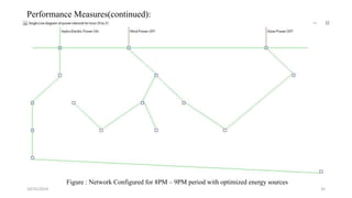
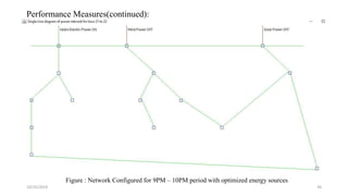
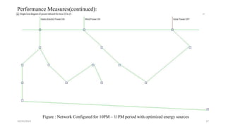
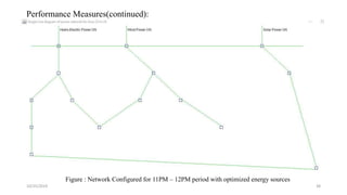

The document presents a genetic algorithm for optimizing dispatching in a microgrid energy system that incorporates renewable sources such as hydro, wind, and solar power. It details the objectives of reducing line loss and operating costs, while matching energy sources to load demands, and outlines a multi-step algorithm involving initialization, evolution through crossover and mutation, and final output of the fittest configuration. The study includes performance evaluations and network configurations that enhance energy resource utilization over a 24-hour period.