The document discusses query processing and optimization. It describes the basic steps in processing an SQL query which includes parsing, translating to relational algebra, optimization to find the most efficient execution plan, and evaluation. The optimizer uses statistical information from system catalogs about relations, attributes, and indexes to estimate the cost of different execution plans and select the most efficient one. The document also covers topics like selection operations, join operations, and methods for estimating the size and cost of different query plans.
![ECS-165A WQ'11 136
8. Query Processing
Goals: Understand the basic concepts underlying the steps in
query processing and optimization and estimating query processing
cost; apply query optimization techniques;
Contents:
Overview
Catalog Information for Cost Estimation
Measures of Query Cost
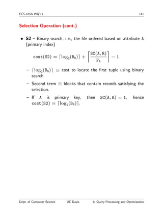
Selection
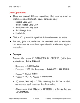
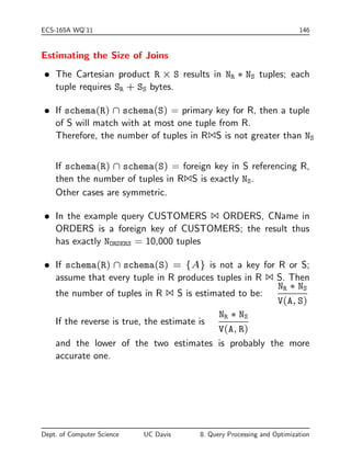
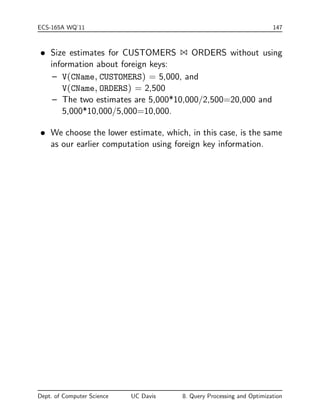
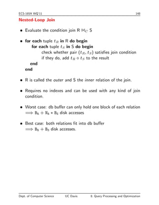
Join Operations
Other Operations
Evaluation and Transformation of Expressions
Query Processing Optimization
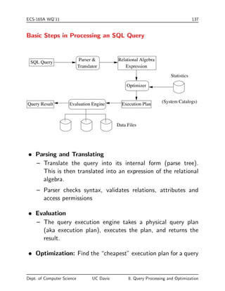
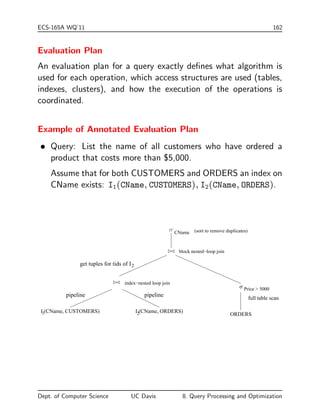
Task: Find an ecient physical query plan (aka execution plan)
for an SQL query
Goal: Minimize the evaluation time for the query, i.e., compute
query result as fast as possible
Cost Factors: Disk accesses, read/write operations, [I/O, page
transfer] (CPU time is typically ignored)
Dept. of Computer Science UC Davis 8. Query Processing and Optimization](https://image.slidesharecdn.com/8-query-141111201009-conversion-gate02/85/8-query-1-320.jpg)
![ECS-165A WQ'11 136
8. Query Processing
Goals: Understand the basic concepts underlying the steps in
query processing and optimization and estimating query processing
cost; apply query optimization techniques;
Contents:
Overview
Catalog Information for Cost Estimation
Measures of Query Cost
Selection
Join Operations
Other Operations
Evaluation and Transformation of Expressions
Query Processing Optimization
Task: Find an ecient physical query plan (aka execution plan)
for an SQL query
Goal: Minimize the evaluation time for the query, i.e., compute
query result as fast as possible
Cost Factors: Disk accesses, read/write operations, [I/O, page
transfer] (CPU time is typically ignored)
Dept. of Computer Science UC Davis 8. Query Processing and Optimization](https://image.slidesharecdn.com/8-query-141111201009-conversion-gate02/75/8-query-1-2048.jpg)