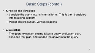
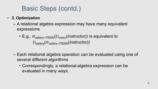
Chapter 5 discusses query processing and optimization, outlining the steps involved in parsing, translating, and evaluating SQL queries to efficient relational algebra expressions. It emphasizes the importance of query optimization to select the lowest cost evaluation plan based on statistical information from the database. The chapter also covers various algorithms for operations, cost estimation for querying, and equivalence rules for transforming relational expressions.

1. Chapter 5:
Query Processing and
Optimization

2. Definitions
• Query processing
– translation of query into low-level activities
– evaluation of query
– data extraction
• Query optimization
– selecting the most efficient query evaluation
2

3. Basic Steps in Query Processing
1. Parsing and translation
2. Optimization
3. Evaluation
3

4. Basic Steps (contd.)
• 1. Parsing and translation
– translate the query into its internal form. This is then translated
into relational algebra.
– Parser checks syntax, verifies relations
• 2. Evaluation
– The query-execution engine takes a query-evaluation plan,
executes that plan, and returns the answers to the query.
4

5. • 3. Optimization
– A relational algebra expression may have many equivalent
expressions
• E.g., salary75000(salary(instructor)) is equivalent to
salary(salary75000(instructor))
– Each relational algebra operation can be evaluated using one of
several different algorithms
• Correspondingly, a relational-algebra expression can be
evaluated in many ways.
5
Basic Steps (contd.)

6. Basic Steps(Cont.)
• Annotated expression specifying detailed evaluation strategy is called
an evaluation-plan.
– E.g., can use an index on salary to find instructors with salary < 75000,
– or can perform complete relation scan and discard instructors with salary  75000
• Query Optimization: Amongst all equivalent evaluation plans choose
the one with lowest cost.
– Cost is estimated using statistical information from the database catalog
• e.g. number of tuples in each relation, size of tuples, etc.
6

7. Query Processing
Example 2: Consider following SQL query, convert it into
equivalent RA query
plans for the query.
and show different query execution
Solution
Equivalent RA query of given SQL query is
5
Sid ,Sname,Cname(Cname'DBMS' (Student ⋈ Enrolls ⋈ Course))
Select Sid, Sname,Cname
From Student Natural Join Enrolls Natural Join Course
Where Cname 'DBMS'
7

8. Query
Execution Plan-1

Processing
Query Query Execution Plan-2

Sid,Sname,Cname Sid,Sname,Cname
 Cname 'DBMS'
Cname 'DBMS'
⋈ ⋈
⋈ ⋈
Course Student
Student Enrolls Enrolls Course
6
8

9. Query
Execution Plan-3

Processing
Query Query Execution Plan-4

Cname 'DBMS' Cname 'DBMS'
Sid,Sname,Cname
Sid,Sname,Cname
⋈ ⋈
⋈ ⋈
Course Student
Student Enrolls Enrolls Course
7
9

10. Measures of Query Cost
• Cost is measured as total elapsed time for answering query
– Many factors contribute to time cost
• disk accesses, CPU, or even network communication
• Typically disk access is the predominant cost, and is also relatively
easy to estimate.
– Measured by taking into account
• Number of seeks * average-seek-cost
• Number of blocks read * average-block-read-cost
• Number of blocks written * average-block-write-cost
– Cost to write a block is greater than cost to read a block
» data is read back after being written to ensure that the write was successful
10

11. Measures of Query Cost (Cont.)
• For simplicity we just use number of block transfers from disk as
the cost measure
– We ignore the difference in cost between sequential and random I/O for
simplicity
– We also ignore CPU costs for simplicity
• Costs depends on the size of the buffer in main memory
– Having more memory reduces need for disk access
– Amount of real memory available to buffer depends on other concurrent OS
processes, and hard to determine ahead of actual execution
– We often use worst case estimates, assuming only the minimum amount of
memory needed for the operation is available
11

12. Measures of Query Cost (Cont.)
• Real systems take CPU cost into account, differentiate between
sequential and random I/O, and take buffer size into account
• We do not include cost to writing output to disk in our cost
formulae
12

13. Selection Operation
• File scan – search algorithms that locate and retrieve records that fulfill a
selection condition.
• Algorithm A1 (linear search). Scan each file block and test all records to see
whether they satisfy the selection condition.
– Cost estimate (number of disk blocks scanned) = br
• br denotes number of blocks containing records from relation r
– If selection is on a key attribute, cost = (br /2)
• stop on finding record
– Linear search can be applied regardless of
• selection condition or
• ordering of records in the file, or
• availability of indices
13

14. Selection Operation (Cont.)
• A2 (binary search). Applicable if selection is an equality
comparison on the attribute on which file is ordered.
– Assume that the blocks of a relation are stored contiguously
– Cost estimate (number of disk blocks to be scanned):
• log2(br) — cost of locating the first tuple by a binary search on the blocks
• Plus number of blocks containing records that satisfy selection condition
14

15. • Alternatives for evaluating an entire expression tree
– Materialization: generate results of an expression whose
inputs are relations or are already computed, materialize
(store) it on disk. Repeat.
– Pipelining: pass on tuples to parent operations even as an
operation is being executed
15

16. Evaluation
• Evaluate multiple operations in a plan
– materialization
– pipelining
16
σcoursename=Advanced DBs
student takes
cid; hash join
courseid; index-nested loop
course
πname

17. Materialization
• create and read temporary relations
• create implies writing to disk
– more page writes
17
σcoursename=Advanced DBs
student takes
cid; hash join
courseid; index-nested loop
course
πname

18. Pipelining
• creating a pipeline of operations
• reduces number of read-write operations
• implementations
– demand-driven - data pull
– producer-driven - data push
18
σcoursename=Advanced DBs
student takes
cid; hash join
ccourseid; index-nested loop
course
πname

19. • In demand driven or lazy evaluation
– system repeatedly requests next tuple from top level operation
– Each operation requests next tuple from children operations as
required, in order to output its next tuple
– In between calls, operation has to maintain “state” so it knows
what to return next
19

20. • In producer-driven or eager pipelining
– Operators produce tuples eagerly and pass them up to their
parents
• Buffer maintained between operators, child puts tuples in buffer, parent
removes tuples from buffer
• if buffer is full, child waits till there is space in the buffer, and then
generates more tuples
– System schedules operations that have space in output buffer and
can process more input tuples
• Alternative name: pull and push models of pipelining
20

21. Query Optimization
• Alternative ways of evaluating a given query
– Equivalent expressions
– Different algorithms for each operation
21

22. Query Optimization (Cont.)
• An evaluation plan defines exactly what algorithm is used for
each operation, and how the execution of the operations is
coordinated.
22
n Find out how to view query execution plans on your favorite database

23. Query Optimization (Cont.)
• Cost difference between evaluation plans for a query can be
enormous
– E.g. seconds vs. days in some cases
• Steps in cost-based query optimization
1.Generate logically equivalent expressions using equivalence rules
2.Annotate resultant expressions to get alternative query plans
3.Choose the cheapest plan based on estimated cost
23

24. Query Optimization (Cont.)
• Estimation of plan cost based on:
– Statistical information about relations. Examples:
• number of tuples, number of distinct values for an attribute
– Statistics estimation for intermediate results to compute cost of
complex expressions
– Cost formulae for algorithms, computed using statistics
24

25. Transformation of Relational Expressions
• Two relational algebra expressions are said to be
equivalent if the two expressions generate the same set
of tuples on every legal database instance
– Note: order of tuples is irrelevant
– we don’t care if they generate different results on databases
that violate integrity constraints
25

26. Transformation of Relational Expressions
(contd.)
• In SQL, inputs and outputs are multisets of tuples
– Two expressions in the multiset version of the relational algebra
are said to be equivalent if the two expressions generate the
same multiset of tuples on every legal database instance.
• An equivalence rule says that expressions of two forms
are equivalent
– Can replace expression of first form by second, or vice versa
26

27. Equivalence Rules
1. Conjunctive selection operations can be deconstructed into a sequence of
individual selections.
2. Selection operations are commutative.
3. Only the last in a sequence of projection operations is needed, the others can
be omitted.
4. Selections can be combined with Cartesian products and theta joins.
a.(E1 X E2) = E1  E2
b.1(E1 2 E2) = E1 1 2 E2
))
(
(
))
(
( 1
2
2
1
E
E 


 


 
)
(
))
))
(
(
(
( 1
2
1
E
E t
tn
t
t 



 K
K
27
))
(
(
)
( 2
1
2
1
E
E 


 

 


28. Equivalence Rules (Cont.)
5. Theta-join operations (and natural joins) are commutative.
E1  E2 = E2  E1
6. (a) Natural join operations are associative:
(E1 E2) E3 = E1 (E2 E3)
(b) Theta joins are associative in the following manner:
(E1 1 E2) 2 3 E3 = E1 1 3 (E2 2 E3)
where 2 involves attributes from only E2 and E3.
28

29. Equivalence Rules (Cont.)
7.The selection operation distributes over the theta join operation under the
following two conditions:
(a) When all the attributes in 0 involve only the attributes of one
of the expressions (E1) being joined.
0E1  E2) = (0(E1))  E2
(b) When  1 involves only the attributes of E1 and 2 involves
only the attributes of E2.
1 E1  E2) = (1(E1))  ( (E2))
29

30. Pictorial Depiction of Equivalence Rules
30

31. Equivalence Rules (Cont.)
8.The projection operation distributes over the theta join operation as follows:
(a) if  involves only attributes from L1  L2:
(b) Consider a join E1  E2.
– Let L1 and L2 be sets of attributes from E1 and E2, respectively.
– Let L3 be attributes of E1 that are involved in join condition , but are not in L1 
L2, and
– let L4 be attributes of E2 that are involved in join condition , but are not in L1 
L2.
31
))
(
(
))
(
(
)
( 2
1
2
1 2
1
2
1
E
E
E
E L
L
L
L 


  

)))
(
(
))
(
((
)
( 2
1
2
1 4
2
3
1
2
1
2
1
E
E
E
E L
L
L
L
L
L
L
L 


 



 


32. Equivalence Rules (Cont.)
9. The set operations union and intersection are commutative
E1  E2 = E2  E1
E1  E2 = E2  E1
n (set difference is not commutative).
10.Set union and intersection are associative.
(E1  E2)  E3 = E1  (E2  E3)
(E1  E2)  E3 = E1  (E2  E3)
11.The selection operation distributes over ,  and –.
 (E1 – E2) =  (E1) – (E2)
and similarly for  and  in place of –
Also:  (E1 – E2) = (E1) – E2
and similarly for  in place of –, but not for 
12. The projection operation distributes over union
L(E1  E2) = (L(E1))  (L(E2))
32

33. • Query: Find the names of all instructors in the Music department, along with the titles of
the courses that they teach
– name, title(dept_name= “Music” (instructor (teaches
course_id, title (course))))
• Transformation using rule 7a.
– name, title((dept_name= “Music”(instructor)) ((teaches course_id, title
(course)))
• Performing the selection as early as possible reduces the size of the relation to be joined.
33

34. 34

35. • Query: Find the names of all instructors in the Music department who have taught a course
in 2009, along with the titles of the courses that they taught
– name, title(dept_name= “Music”year = 2009
(instructor (teaches course_id, title (course))))
• Transformation using join associatively (Rule 6a):
– name, title(dept_name= “Music”gear = 2009
((instructor teaches) course_id, title (course)))
• Second form provides an opportunity to apply the “perform selections early” rule, resulting in
the subexpression
dept_name = “Music” (instructor)  year = 2009 (teaches)
35

36. Multiple Transformations (Cont.)
36

37. • Consider: name, title(dept_name= “Music” (instructor) teaches)
course_id, title (course))))
• When we compute
(dept_name = “Music” (instructor teaches)
we obtain a relation whose schema is:
(ID, name, dept_name, salary, course_id, sec_id, semester, year)
• Push projections using equivalence rules 8a and 8b; eliminate unneeded attributes from
intermediate results to get:
name, title(name, course_id (
dept_name= “Music” (instructor) teaches))
course_id, title (course))))
• Performing the projection as early as possible reduces the size of the relation to be joined.
37

38. Evaluation Plan
• An evaluation plan defines exactly what algorithm is used for each
operation, and how the execution of the operations is coordinated.
38

39. Choice of Evaluation Plans
• Must consider the interaction of evaluation techniques when choosing
evaluation plans: choosing the cheapest algorithm for each operation
independently may not yield best overall algorithm. E.g.
– merge-join may be costlier than hash-join, but may provide a sorted output which reduces
the cost for an outer level aggregation.
– nested-loop join may provide opportunity for pipelining
• Practical query optimizers incorporate elements of the following two broad
approaches:
1. Search all the plans and choose the best plan in a cost-based fashion.
2. Uses heuristics to choose a plan.
39

40. Cost-Based Optimization
• Consider finding the best join-order for r1 r2 . . . rn.
• There are (2(n – 1))!/(n – 1)! different join orders for above
expression. With n = 7, the number is 665280, with n = 10,
the number is greater than 176 billion!
• No need to generate all the join orders. Using dynamic
programming, the least-cost join order for any subset of
{r1, r2, . . . rn} is computed only once and stored for future use.
40

41. Cost Estimation
• Cost of each operator computed
– Need statistics of input relations
• E.g. number of tuples, sizes of tuples
• Inputs can be results of sub-expressions
– Need to estimate statistics of expression results
– To do so, we require additional statistics
• E.g. number of distinct values for an attribute
41

42. Left Deep Join Trees
• In left-deep join trees, the right-hand-side input for each join is a
relation, not the result of an intermediate join.
42

43. Cost of Optimization
• With dynamic programming time complexity of optimization with bushy trees
is O(3n).
– With n = 10, this number is 59000 instead of 176 billion!
• Space complexity is O(2n)
• To find best left-deep join tree for a set of n relations:
– Consider n alternatives with one relation as right-hand side input and the other relations
as left-hand side input.
– Using (recursively computed and stored) least-cost join order for each alternative on left-
hand-side, choose the cheapest of the n alternatives.
• If only left-deep trees are considered, time complexity of finding best join
order is O(n 2n)
– Space complexity remains at O(2n)
• Cost-based optimization is expensive, but worthwhile for queries on large
datasets (typical queries have small n, generally < 10)
43

44. Interesting Orders in Cost-Based Optimization
• Consider the expression (r1 r2 r3) r4 r5
• An interesting sort order is a particular sort order of tuples that could be
useful for a later operation.
– Generating the result of r1 r2 r3 sorted on the attributes common with r4 or r5 may be
useful, but generating it sorted on the attributes common only r1 and r2 is not useful.
– Using merge-join to compute r1 r2 r3 may be costlier, but may provide an output
sorted in an interesting order.
• Not sufficient to find the best join order for each subset of the set of n given
relations; must find the best join order for each subset, for each interesting
sort order
– Simple extension of earlier dynamic programming algorithms
– Usually, number of interesting orders is quite small and doesn’t affect time/space
complexity significantly
44

45. Heuristic Optimization
• Cost-based optimization is expensive, even with dynamic programming.
• Systems may use heuristics to reduce the number of choices that must be
made in a cost-based fashion.
• Heuristic optimization transforms the query-tree by using a set of rules that
typically (but not in all cases) improve execution performance:
– Perform selection early (reduces the number of tuples)
– Perform projection early (reduces the number of attributes)
– Perform most restrictive selection and join operations before other similar operations.
– Some systems use only heuristics, others combine heuristics with partial cost-based
optimization.
45

46. Steps in Typical Heuristic Optimization
1. Deconstruct conjunctive selections into a sequence of single selection operations
(Equiv. rule 1.).
2. Move selection operations down the query tree for the earliest possible execution
(Equiv. rules 2, 7a, 7b, 11).
3. Execute first those selection and join operations that will produce the smallest
relations (Equiv. rule 6).
4. Replace Cartesian product operations that are followed by a selection condition
by join operations (Equiv. rule 4a).
5. Deconstruct and move as far down the tree as possible lists of projection
attributes, creating new projections where needed (Equiv. rules 3, 8a, 8b, 12).
6. Identify those subtrees whose operations can be pipelined, and execute them
using pipelining).
46