dbms notes

1. I
Query processing and optimization: Evaluation of
relational algebra expressions, Query equivalence, Join
strategies,
PRESENTED BY :
SARABJIT KAUR
ASSITANT PROFESSOR
Department of CSE
IKGPTU , KAPURTHALA

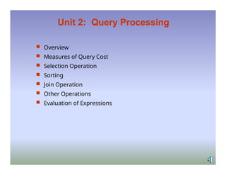
2. Unit 2: Query Processing
 Overview
 Measures of Query Cost
 Selection Operation
 Sorting
 Join Operation
 Other Operations
 Evaluation of Expressions

3. Basic Steps in Query Processing
1. Parsing and
translation
2. Optimization
3. Evaluation

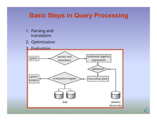
4. Basic Steps in Query Processing
(Cont.)
 Parsing and translation
🟊translate the query into its internal form.
This is then translated into relational
algebra.
🟊Parser checks syntax, verifies relations
 Evaluation
🟊The query-execution engine takes a query-
evaluation plan, executes that plan, and returns
the answers to the query.

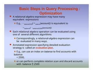
5. Basic Steps in Query Processing :
Optimization
 A relational algebra expression may have many
equivalent expressions
🟊 E.g., balance2500(balance(account)) is equivalent to
balance(balance2500(account))
 Each relational algebra operation can be evaluated using
one of several different algorithms
🟊 Correspondingly, a relational-algebra expression can
be evaluated in many ways.
 Annotated expression specifying detailed evaluation
strategy is called an evaluation-plan.
🟊 E.g., can use an index on balance to find accounts with
balance
< 2500,
🟊 or can perform complete relation scan and discard accounts
with balance  2500

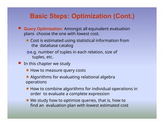
6. Basic Steps: Optimization (Cont.)
 Query Optimization: Amongst all equivalent evaluation
plans choose the one with lowest cost.
🟊 Cost is estimated using statistical information from
the database catalog
e.g. number of tuples in each relation, size of
tuples, etc.
 In this chapter we study
🟊 How to measure query costs
🟊 Algorithms for evaluating relational algebra
operations
🟊 How to combine algorithms for individual operations in
order to evaluate a complete expression
🟊 We study how to optimize queries, that is, how to
find an evaluation plan with lowest estimated cost

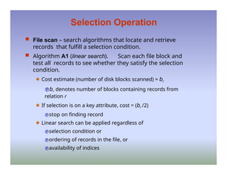
7. Selection Operation
 File scan – search algorithms that locate and retrieve
records that fulfill a selection condition.
 Algorithm A1 (linear search). Scan each file block and
test all records to see whether they satisfy the selection
condition.
🟊 Cost estimate (number of disk blocks scanned) = br
br denotes number of blocks containing records from
relation r
🟊 If selection is on a key attribute, cost = (br /2)
stop on finding record
🟊 Linear search can be applied regardless of
selection condition or
ordering of records in the file, or
availability of indices

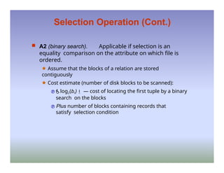
8. Selection Operation (Cont.)
 A2 (binary search). Applicable if selection is an
equality comparison on the attribute on which file is
ordered.
🟊 Assume that the blocks of a relation are stored
contiguously
🟊 Cost estimate (number of disk blocks to be scanned):
log2(br) — cost of locating the first tuple by a binary
search on the blocks
 Plus number of blocks containing records that
satisfy selection condition

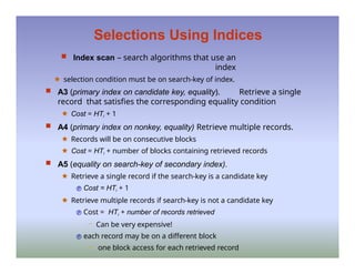
9. Selections Using Indices
 Index scan – search algorithms that use an
index
🟊 selection condition must be on search-key of index.
 A3 (primary index on candidate key, equality). Retrieve a single
record that satisfies the corresponding equality condition
🟊 Cost = HTi + 1
 A4 (primary index on nonkey, equality) Retrieve multiple records.
🟊 Records will be on consecutive blocks
🟊 Cost = HTi + number of blocks containing retrieved records
 A5 (equality on search-key of secondary index).
🟊 Retrieve a single record if the search-key is a candidate key
 Cost = HTi + 1
🟊 Retrieve multiple records if search-key is not a candidate key
 Cost = HTi + number of records retrieved
– Can be very expensive!
 each record may be on a different block
– one block access for each retrieved record

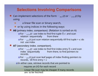
10. Selections Involving Comparisons
 Can implement selections of the form AV (r) or A  V(r) by
using
🟊 a linear file scan or binary search,
🟊 or by using indices in the following ways:
 A6 (primary index, comparison). (Relation is sorted on A)
For A  V(r) use index to find first tuple  v and scan
relation sequentially from there
For AV (r) just scan relation sequentially till first tuple > v; do
not use index
 A7 (secondary index, comparison).
For A  V(r) use index to find first index entry  v and scan
index sequentially from there, to find pointers to
records.
For AV (r) just scan leaf pages of index finding pointers to
records, till first entry > v
In either case, retrieve records that are pointed to
– requires an I/O for each record
– Linear file scan may be cheaper if many records
are to be fetched!

11. Sorting
 We may build an index on the relation, and then use the
index to read the relation in sorted order. May lead to
one disk block access for each tuple.
 For relations that fit in memory, techniques like quicksort
can be used. For relations that don’t fit in memory,
external
sort-merge is a good choice.

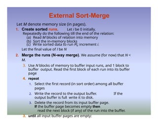
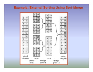
12. External Sort-Merge
Let M denote memory size (in pages).
1. Create sorted runs. Let i be 0 initially.
Repeatedly do the following till the end of the relation:
(a) Read M blocks of relation into memory
(b) Sort the in-memory blocks
(c) Write sorted data to run Ri; increment i.
Let the final value of I be N
2. Merge the runs (N-way merge). We assume (for now) that N <
M.
3. Use N blocks of memory to buffer input runs, and 1 block to
buffer output. Read the first block of each run into its buffer
page
4. repeat
1. Select the first record (in sort order) among all buffer
pages
2. Write the record to the output buffer. If the
output buffer is full write it to disk.
3. Delete the record from its input buffer page.
If the buffer page becomes empty then
read the next block (if any) of the run into the buffer.
3. until all input buffer pages are empty:

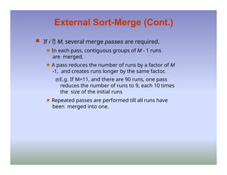
13. External Sort-Merge (Cont.)
 If i  M, several merge passes are required.
🟊 In each pass, contiguous groups of M - 1 runs
are merged.
🟊 A pass reduces the number of runs by a factor of M
-1, and creates runs longer by the same factor.
E.g. If M=11, and there are 90 runs, one pass
reduces the number of runs to 9, each 10 times
the size of the initial runs
🟊 Repeated passes are performed till all runs have
been merged into one.

14. Example: External Sorting Using Sort-Merge

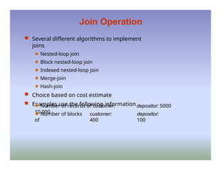
15. Join Operation
 Several different algorithms to implement
joins
🟊 Nested-loop join
🟊 Block nested-loop join
🟊 Indexed nested-loop join
🟊 Merge-join
🟊 Hash-join
 Choice based on cost estimate
 Examples use the following information
🟊 Number of records of customer:
10,000
🟊 Number of blocks
of
customer:
400
depositor: 5000
depositor:
100

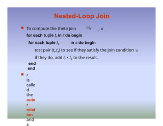
16. Nested-Loop Join
 To compute the theta join r  s
for each tuple tr in r do begin
for each tuple ts in s do begin
test pair (tr,ts) to see if they satisfy the join condition 
if they do, add tr • ts to the result.
end
end
 r
is
calle
d
the
oute
r
relat
ion
and
s

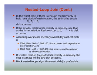
17. Nested-Loop Join (Cont.)
 In the worst case, if there is enough memory only to
hold one block of each relation, the estimated cost is
nr  bs + br
disk accesses.
 If the smaller relation fits entirely in memory, use that
as the inner relation. Reduces cost to br + bs disk
accesses.
 Assuming worst case memory availability cost estimate
is
🟊 5000  400 + 100 = 2,000,100 disk accesses with depositor as
outer relation, and
🟊 1000  100 + 400 = 1,000,400 disk accesses with customer
as the outer relation.
 If smaller relation (depositor) fits entirely in memory, the
cost estimate will be 500 disk accesses.
 Block nested-loops algorithm (next slide) is preferable.

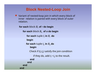
18. Block Nested-Loop Join
 Variant of nested-loop join in which every block of
inner relation is paired with every block of outer
relation.
for each block Br of r do begin
for each block Bs of s do begin
for each tuple tr in Br do
begin
for each tuple ts in Bs do
begin
Check if (tr,ts) satisfy the join condition
if they do, add tr • ts to the result.
end
end
end
end

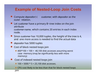
19. Example of Nested-Loop Join Costs
 Compute depositor customer, with depositor as the
outer relation.
 Let customer have a primary B+-tree index on the join
attribute
customer-name, which contains 20 entries in each index
node.
 Since customer has 10,000 tuples, the height of the tree is 4,
and one more access is needed to find the actual data
 depositor has 5000 tuples
 Cost of block nested loops join
🟊 400*100 + 100 = 40,100 disk accesses assuming worst
case memory (may be significantly less with more
memory)
 Cost of indexed nested loops join
🟊 100 + 5000 * 5 = 25,100 disk accesses.
🟊 CPU cost likely to be less than that for block nested loops
join

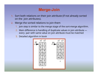
20. Merge-Join
1. Sort both relations on their join attribute (if not already sorted
on the join attributes).
2. Merge the sorted relations to join them
1. Join step is similar to the merge stage of the sort-merge algorithm.
2. Main difference is handling of duplicate values in join attribute —
every pair with same value on join attribute must be matched
3. Detailed algorithm in book

21. Merge-Join (Cont.)
 Can be used only for equi-joins and natural joins
 Each block needs to be read only once (assuming all tuples
for any given value of the join attributes fit in memory
 Thus number of block accesses for merge-join is
br + bs + the cost of sorting if relations are
unsorted.
 hybrid merge-join: If one relation is sorted, and the other
has a secondary B+-tree index on the join attribute
🟊 Merge the sorted relation with the leaf entries of the B+-tree .
🟊 Sort the result on the addresses of the unsorted relation’s
tuples
🟊 Scan the unsorted relation in physical address order and merge
with previous result, to replace addresses by the actual tuples
Sequential scan more efficient than random lookup

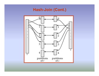
22. Hash-Join
 Applicable for equi-joins and natural joins.
 A hash function h is used to partition tuples of both
relations
 h maps JoinAttrs values to {0, 1, ..., n}, where JoinAttrs
denotes the common attributes of r and s used in the
natural join.
🟊 r0, r1, . . ., rn denote partitions of r tuples
Each tuple tr  r is put in partition ri where i = h(tr
[JoinAttrs]).
🟊 r0,, r1. . ., rn denotes partitions of s tuples
Each tuple ts s is put in partition si, where i = h(ts
[JoinAttrs]).
 Note: In book, ri is denoted as Hri, si is denoted as Hsi
and
n is denoted as n

23. Hash-Join (Cont.)

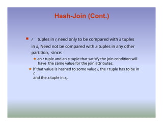
24. Hash-Join (Cont.)
 r tuples in ri need only to be compared with s tuples
in si Need not be compared with s tuples in any other
partition, since:
🟊 an r tuple and an s tuple that satisfy the join condition will
have the same value for the join attributes.
🟊 If that value is hashed to some value i, the r tuple has to be in
ri
and the s tuple in si.

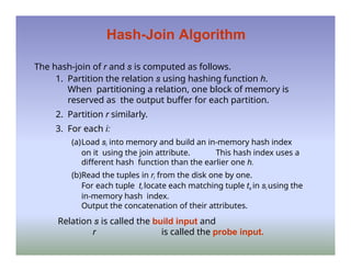
25. Hash-Join Algorithm
The hash-join of r and s is computed as follows.
1. Partition the relation s using hashing function h.
When partitioning a relation, one block of memory is
reserved as the output buffer for each partition.
2. Partition r similarly.
3. For each i:
(a)Load si into memory and build an in-memory hash index
on it using the join attribute. This hash index uses a
different hash function than the earlier one h.
(b)Read the tuples in ri from the disk one by one.
For each tuple tr locate each matching tuple ts in si using the
in-memory hash index.
Output the concatenation of their attributes.
Relation s is called the build input and
r is called the probe input.

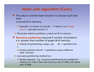
26. Hash-Join algorithm (Cont.)
 The value n and the hash function h is chosen such that
each
si should fit in memory.
🟊 Typically n is chosen as bs/M * f where f is a “fudge
factor”, typically around 1.2
🟊 The probe relation partitions si need not fit in memory
 Recursive partitioning required if number of partitions
n is greater than number of pages M of memory.
🟊 instead of partitioning n ways, use M – 1 partitions for
s
🟊 Further partition the M – 1 partitions using a different
hash function
🟊 Use same partitioning method on r
🟊 Rarely required: e.g., recursive partitioning not needed for
relations of 1GB or less with memory size of 2MB, with block
size of 4KB.

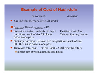
27. Example of Cost of Hash-Join
customer depositor
 Assume that memory size is 20 blocks
 bdepositor= 100 and bcustomer = 400.
 depositor is to be used as build input. Partition it into five
partitions, each of size 20 blocks. This partitioning can be
done in one pass.
 Similarly, partition customer into five partitions,each of size
80. This is also done in one pass.
 Therefore total cost: 3(100 + 400) = 1500 block transfers
🟊 ignores cost of writing partially filled blocks

28. Hybrid Hash–Join
 Useful when memory sized are relatively large, and the build
input is bigger than memory.
 Main feature of hybrid hash join:
Keep the first partition of the build relation in memory.
 E.g. With memory size of 25 blocks, depositor can be
partitioned into five partitions, each of size 20 blocks.
 Division of memory:
🟊 The first partition occupies 20 blocks of memory
🟊 1 block is used for input, and 1 block each for buffering the
other 4 partitions.
 customer is similarly partitioned into five partitions each of size
80; the first is used right away for probing, instead of being
written out and read back.
 Cost of 3(80 + 320) + 20 +80 = 1300 block transfers
for hybrid hash join, instead of 1500 with plain
hash-join.
 Hybrid hash-join most useful if M
>>
bs

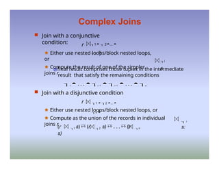
29. Complex Joins
 Join with a conjunctive
condition: r 1  2... 
 n s
🟊 Either use nested loops/block nested loops,
or
🟊 Compute the result of one of the simpler
joins r
i
s
final result comprises those tuples in the intermediate
result that satisfy the remaining conditions
1  . . .  i –1  i +1  . . .  n
 Join with a disjunctive condition
r 1  2 ... 
n s
🟊 Either use nested loops/block nested loops, or
🟊 Compute as the union of the records in individual
joins r
 i
s:
(r 1 s)  (r 2 s)  . . .  (r n
s)

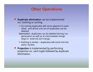
30. Other Operations
 Duplicate elimination can be implemented
via hashing or sorting.
🟊 On sorting duplicates will come adjacent to each
other, and all but one set of duplicates can be
deleted.
Optimization: duplicates can be deleted during run
generation as well as at intermediate merge
steps in external sort-merge.
🟊 Hashing is similar – duplicates will come into the
same bucket.
 Projection is implemented by performing
projection on each tuple followed by duplicate
elimination.

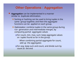
31. Other Operations : Aggregation
 Aggregation can be implemented in a manner
similar to duplicate elimination.
🟊 Sorting or hashing can be used to bring tuples in the
same group together, and then the aggregate
functions can be applied on each group.
🟊 Optimization: combine tuples in the same group during
run generation and intermediate merges, by
computing partial aggregate values
For count, min, max, sum: keep aggregate values
on tuples found so far in the group.
– When combining partial aggregate for count,
add up the aggregates
For avg, keep sum and count, and divide sum by
count at the end

32. Other Operations : Set Operations
 Set operations (,  and ): can either use
variant of merge-join after sorting, or variant of
hash-join.
 E.g., Set operations using hashing:
1. Partition both relations using the same hash function,
thereby
creating, r1, .., rn r0, and s1, s2.., sn
2. Process each partition i as follows. Using a different
hashing function, build an in-memory hash index on ri
after it is brought into memory.
3. – r  s: Add tuples in si to the hash index if they are not
already in it. At end of si add the tuples in the hash index to
the result.
– r  s: output tuples in si to the result if they are already
there in the hash index.
– r – s: for each tuple in si, if it is there in the hash index,
delete it from the index. At end of si add remaining tuples
in the hash index to the result.

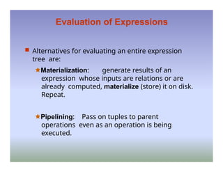
33. Evaluation of Expressions
 Alternatives for evaluating an entire expression
tree are:
🟊Materialization: generate results of an
expression whose inputs are relations or are
already computed, materialize (store) it on disk.
Repeat.
🟊Pipelining: Pass on tuples to parent
operations even as an operation is being
executed.

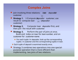
34. Complex Joins
 Join involving three relations: loan depositor
customer
 Strategy 1. Compute depositor customer; use
result to compute loan (depositor
customer)
 Strategy 2. Computer loan depositor first, and
then join the result with customer.
 Strategy 3. Perform the pair of joins at once.
Build and index on loan for loan-number, and on
customer for customer-name.
🟊 For each tuple t in depositor, look up the corresponding
tuples in customer and the corresponding tuples in loan.
🟊 Each tuple of deposit is examined exactly once.
 Strategy 3 combines two operations into one special-
purpose operation that is more efficient than
implementing two joins of two relations.

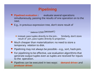
35. Pipelining
 Pipelined evaluation : evaluate several operations
simultaneously, passing the results of one operation on to the
next.
 E.g., in previous expression tree, don’t store result of
 balance 2500 (account )
🟊 instead, pass tuples directly to the join.. Similarly, don’t store
result of join, pass tuples directly to projection.
 Much cheaper than materialization: no need to store a
temporary relation to disk.
 Pipelining may not always be possible – e.g., sort, hash-join.
 For pipelining to be effective, use evaluation algorithms that
generate output tuples even as tuples are received for inputs
to the operation.
 Pipelines can be executed in two ways: demand driven and
producer driven

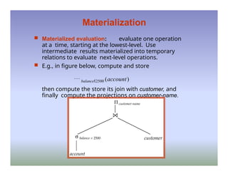
36. Materialization
 Materialized evaluation: evaluate one operation
at a time, starting at the lowest-level. Use
intermediate results materialized into temporary
relations to evaluate next-level operations.
 E.g., in figure below, compute and store
balance2500 (account)
then compute the store its join with customer, and
finally compute the projections on customer-name.

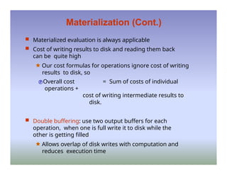
37. Materialization (Cont.)
 Materialized evaluation is always applicable
 Cost of writing results to disk and reading them back
can be quite high
🟊 Our cost formulas for operations ignore cost of writing
results to disk, so
Overall cost = Sum of costs of individual
operations +
cost of writing intermediate results to
disk.
 Double buffering: use two output buffers for each
operation, when one is full write it to disk while the
other is getting filled
🟊 Allows overlap of disk writes with computation and
reduces execution time