R programming by ganesh kavhar

R-programming
Presented by
ganesh kavhar

Outline
• Introduction:
– Historical development
– S, Splus
– Capability
– Statistical Analysis
• References
• Calculator
• Data Type
• Resources
• Simulation and Statistical
Tables
– Probability distributions
• Programming
– Grouping, loops and conditional
execution
– Function
• Reading and writing data from
files
• Modeling
– Regression
– ANOVA
• Data Analysis on Association
–Lottery
–Geyser
• Smoothing

R, S and S-plus
• S: an interactive environment for data analysis developed at Bell
Laboratories since 1976
– 1988 - S2: RA Becker, JM Chambers, A Wilks
– 1992 - S3: JM Chambers, TJ Hastie
– 1998 - S4: JM Chambers
• Exclusively licensed by AT&T/Lucent to Insightful Corporation,
Seattle WA. Product name: “S-plus”.
• Implementation languages C, Fortran.
• See:
http://cm.bell-labs.com/cm/ms/departments/sia/S/history.html
• R: initially written by Ross Ihaka and Robert Gentleman at Dep.
of Statistics of U of Auckland, New Zealand during 1990s.
• Since 1997: international “R-core” team of ca. 15 people with
access to common CVS archive.

Introduction
•R is “GNU S” — A language and environment for data manipula-
tion, calculation and graphical display.
– R is similar to the award-winning S system, which was developed at Bell
Laboratories by John Chambers et al.
– a suite of operators for calculations on arrays, in particular matrices,
– a large, coherent, integrated collection of intermediate tools for interactive data
analysis,
– graphical facilities for data analysis and display either directly at the computer
or on hardcopy
– a well developed programming language which includes conditionals, loops,
user defined recursive functions and input and output facilities.
•The core of R is an interpreted computer language.
– It allows branching and looping as well as modular programming using
functions.
– Most of the user-visible functions in R are written in R, calling upon a smaller
set of internal primitives.
– It is possible for the user to interface to procedures written in C, C++ or
FORTRAN languages for efficiency, and also to write additional primitives.

What R does and does not
odata handling and storage:
numeric, textual
omatrix algebra
ohash tables and regular
expressions
ohigh-level data analytic and
statistical functions
oclasses (“OO”)
ographics
oprogramming language:
loops, branching,
subroutines
ois not a database, but
connects to DBMSs
ohas no graphical user
interfaces, but connects to
Java, TclTk
olanguage interpreter can be
very slow, but allows to call
own C/C++ code
ono spreadsheet view of data,
but connects to
Excel/MsOffice
ono professional /
commercial support

R and statistics
o Packaging: a crucial infrastructure to efficiently produce, load
and keep consistent software libraries from (many) different
sources / authors
o Statistics: most packages deal with statistics and data analysis
o State of the art: many statistical researchers provide their
methods as R packages

Data Analysis and Presentation
• The R distribution contains functionality for large number of
statistical procedures.
– linear and generalized linear models
– nonlinear regression models
– time series analysis
– classical parametric and nonparametric tests
– clustering
– smoothing
• R also has a large set of functions which provide a flexible
graphical environment for creating various kinds of data
presentations.

References
• For R,
– The basic reference is The New S Language: A Programming Environment
for Data Analysis and Graphics by Richard A. Becker, John M. Chambers
and Allan R. Wilks (the “Blue Book”) .
– The new features of the 1991 release of S (S version 3) are covered in
Statistical Models in S edited by John M. Chambers and Trevor J. Hastie
(the “White Book”).
– Classical and modern statistical techniques have been implemented.
• Some of these are built into the base R environment.
• Many are supplied as packages. There are about 8 packages supplied with R
(called “standard” packages) and many more are available through the cran
family of Internet sites (via http://cran.r-project.org).
• All the R functions have been documented in the form of help
pages in an “output independent” form which can be used to create
versions for HTML, LATEX, text etc.
– The document “An Introduction to R” provides a more user-friendly starting
point.
– An “R Language Definition” manual
– More specialized manuals on data import/export and extending R.

R as a calculator
> log2(32)
[1] 5
> sqrt(2)
[1] 1.414214
> seq(0, 5, length=6)
[1] 0 1 2 3 4 5
> plot(sin(seq(0, 2*pi, length=100)))
0 20 40 60 80 100
-1.0-0.50.00.51.0
Index
sin(seq(0,2*pi,length=100))

Object orientation
primitive (or: atomic) data types in R are:
• numeric (integer, double, complex)
• character
• logical
• function
out of these, vectors, arrays, lists can be built.

Object orientation
• Object: a collection of atomic variables and/or other objects that
belong together
• Example: a microarray experiment
• probe intensities
• patient data (tissue location, diagnosis, follow-up)
• gene data (sequence, IDs, annotation)
Parlance:
• class: the “abstract” definition of it
• object: a concrete instance
• method: other word for ‘function’
• slot: a component of an object

Object orientation
Advantages:
Encapsulation (can use the objects and methods someone else has
written without having to care about the internals)
Generic functions (e.g. plot, print)
Inheritance (hierarchical organization of complexity)
Caveat:
Overcomplicated, baroque program architecture…

variables
> a = 49
> sqrt(a)
[1] 7
> a = "The dog ate my homework"
> sub("dog","cat",a)
[1] "The cat ate my homework“
> a = (1+1==3)
> a
[1] FALSE
numeric
character
string
logical

vectors, matrices and arrays
• vector: an ordered collection of data of the same type
> a = c(1,2,3)
> a*2
[1] 2 4 6
• Example: the mean spot intensities of all 15488 spots on a chip:
a vector of 15488 numbers
• In R, a single number is the special case of a vector with 1
element.
• Other vector types: character strings, logical

vectors, matrices and arrays
• matrix: a rectangular table of data of the same type
• example: the expression values for 10000 genes for 30 tissue
biopsies: a matrix with 10000 rows and 30 columns.
• array: 3-,4-,..dimensional matrix
• example: the red and green foreground and background values
for 20000 spots on 120 chips: a 4 x 20000 x 120 (3D) array.

Lists
• vector: an ordered collection of data of the same type.
> a = c(7,5,1)
> a[2]
[1] 5
• list: an ordered collection of data of arbitrary types.
> doe = list(name="john",age=28,married=F)
> doe$name
[1] "john“
> doe$age
[1] 28
• Typically, vector elements are accessed by their index (an integer),
list elements by their name (a character string). But both types
support both access methods.

Data frames
data frame: is supposed to represent the typical data table that
researchers come up with – like a spreadsheet.
It is a rectangular table with rows and columns; data within each
column has the same type (e.g. number, text, logical), but
different columns may have different types.
Example:
> a
localisation tumorsize progress
XX348 proximal 6.3 FALSE
XX234 distal 8.0 TRUE
XX987 proximal 10.0 FALSE

Factors
A character string can contain arbitrary text. Sometimes it is useful to use a limited
vocabulary, with a small number of allowed words. A factor is a variable that can only
take such a limited number of values, which are called levels.
> a
[1] Kolon(Rektum) Magen Magen
[4] Magen Magen Retroperitoneal
[7] Magen Magen(retrogastral) Magen
Levels: Kolon(Rektum) Magen Magen(retrogastral) Retroperitoneal
> class(a)
[1] "factor"
> as.character(a)
[1] "Kolon(Rektum)" "Magen" "Magen"
[4] "Magen" "Magen" "Retroperitoneal"
[7] "Magen" "Magen(retrogastral)" "Magen"
> as.integer(a)
[1] 1 2 2 2 2 4 2 3 2
> as.integer(as.character(a))
[1] NA NA NA NA NA NA NA NA NA NA NA NA
Warning message: NAs introduced by coercion

Subsetting
Individual elements of a vector, matrix, array or data frame are
accessed with “[ ]” by specifying their index, or their name
> a
XX348 proximal 6.3 0
XX234 distal 8.0 1
> a[3, 2]
[1] 10
> a["XX987", "tumorsize"]
[1] 10
> a["XX987",]
XX987 proximal 10 0

SubsettingSubsetting
> a
XX234 distal 8.0 1
> a[c(1,3),]
> a[c(T,F,T),]
> a$localisation
[1] "proximal" "distal" "proximal"
> a$localisation=="proximal"
[1] TRUE FALSE TRUE
> a[ a$localisation=="proximal", ]
subset rows by a
vector of indices
subset rows by a
logical vector
subset a column
comparison resulting in
logical vector
subset the selected
rows

Resources
• A package specification allows the production of loadable modules
for specific purposes, and several contributed packages are made
available through the CRAN sites.
• CRAN and R homepage:
– http://www.r-project.org/
It is R’s central homepage, giving information on the R project and
everything related to it.
– http://cran.r-project.org/
It acts as the download area,carrying the software itself, extension packages,
PDF manuals.
• Getting help with functions and features
– help(solve)
– ?solve
– For a feature specified by special characters, the argument must be enclosed
in double or single quotes, making it a “character string”: help("[[")

Getting help
Details about a specific command whose name you know (input
arguments, options, algorithm, results):
>? t.test
or
>help(t.test)

Getting help
o HTML search engine
o Search for topics
with regular
expressions:
“help.search”

Probability distributions
• Cumulative distribution function P(X ≤ x): ‘p’ for the CDF
• Probability density function: ‘d’ for the density,,
• Quantile function (given q, the smallest x such that P(X ≤ x) > q):
‘q’ for the quantile
• simulate from the distribution: ‘r
Distribution R name additional arguments
beta beta shape1, shape2, ncp
binomial binom size, prob
Cauchy cauchy location, scale
chi-squared chisq df, ncp
exponential exp rate
F f df1, df1, ncp
gamma gamma shape, scale
geometric geom prob
hypergeometric hyper m, n, k
log-normal lnorm meanlog, sdlog
logistic logis; negative binomial nbinom; normal norm; Poisson pois; Student’s t
t ; uniform unif; Weibull weibull; Wilcoxon wilcox

Grouping, loops and conditional execution
• Grouped expressions
– R is an expression language in the sense that its only command type is a
function or expression which returns a result.
– Commands may be grouped together in braces, {expr 1, . . ., expr m}, in
which case the value of the group is the result of the last expression in the
group evaluated.
• Control statements
– if statements
– The language has available a conditional construction of the form
if (expr 1) expr 2 else expr 3
where expr 1 must evaluate to a logical value and the result of the entire
expression is then evident.
– a vectorized version of the if/else construct, the ifelse function. This has the
form ifelse(condition, a, b)

Repetitive execution
• for loops, repeat and while
–for (name in expr 1) expr 2
where name is the loop variable. expr 1 is a vector expression,
(often a sequence like 1:20), and expr 2 is often a grouped
expression with its sub-expressions written in terms of the
dummy name. expr 2 is repeatedly evaluated as name ranges
through the values in the vector result of expr 1.
• Other looping facilities include the
–repeat expr statement and the
–while (condition) expr statement.
–The break statement can be used to terminate any loop, possibly
abnormally. This is the only way to terminate repeat loops.
–The next statement can be used to discontinue one particular
cycle and skip to the “next”.

Branching
if (logical expression) {
statements
} else {
alternative statements
}
else branch is optional

Loops
• When the same or similar tasks need to be performed multiple
times; for all elements of a list; for all columns of an array; etc.
• Monte Carlo Simulation
• Cross-Validation (delete one and etc)
for(i in 1:10) {
print(i*i)
}
i=1
while(i<=10) {
print(i*i)
i=i+sqrt(i)
}

lapply, sapply, apply
• When the same or similar tasks need to be performed multiple
times for all elements of a list or for all columns of an array.
• May be easier and faster than “for” loops
• lapply(li, function )
• To each element of the list li, the function function is applied.
• The result is a list whose elements are the individual function
results.
> li = list("klaus","martin","georg")
> lapply(li, toupper)
> [[1]]
> [1] "KLAUS"
> [[2]]
> [1] "MARTIN"
> [[3]]
> [1] "GEORG"

lapply, sapply, apply
sapply( li, fct )
Like apply, but tries to simplify the result, by converting it into a
vector or array of appropriate size
> li = list("klaus","martin","georg")
> sapply(li, toupper)
[1] "KLAUS" "MARTIN" "GEORG"
> fct = function(x) { return(c(x, x*x, x*x*x)) }
> sapply(1:5, fct)
[,1] [,2] [,3] [,4] [,5]
[1,] 1 2 3 4 5
[2,] 1 4 9 16 25
[3,] 1 8 27 64 125

apply
apply( arr, margin, fct )
Apply the function fct along some dimensions of the array arr,
according to margin, and return a vector or array of the
appropriate size.
> x
[,1] [,2] [,3]
[1,] 5 7 0
[2,] 7 9 8
[3,] 4 6 7
[4,] 6 3 5
> apply(x, 1, sum)
[1] 12 24 17 14
> apply(x, 2, sum)
[1] 22 25 20

functions and operators
Functions do things with data
“Input”: function arguments (0,1,2,…)
“Output”: function result (exactly one)
Example:
add = function(a,b)
{ result = a+b
return(result) }
Operators:
Short-cut writing for frequently used functions of one or two
arguments.
Examples: + - * / ! & | %%

functions and operators
• Functions do things with data
• “Input”: function arguments (0,1,2,…)
• “Output”: function result (exactly one)
Exceptions to the rule:
• Functions may also use data that sits around in other places, not
just in their argument list: “scoping rules”*
• Functions may also do other things than returning a result. E.g.,
plot something on the screen: “side effects”
* Lexical scope and Statistical Computing.
R. Gentleman, R. Ihaka, Journal of Computational and
Graphical Statistics, 9(3), p. 491-508 (2000).

Reading data from files
• The read.table() function
– To read an entire data frame directly, the external file will normally have a
special form.
– The first line of the file should have a name for each variable in the data
frame.
– Each additional line of the file has its first item a row label and the values for
each variable.
Price Floor Area Rooms Age Cent.heat
01 52.00 111.0 830 5 6.2 no
02 54.75 128.0 710 5 7.5 no
03 57.50 101.0 1000 5 4.2 no
04 57.50 131.0 690 6 8.8 no
05 59.75 93.0 900 5 1.9 yes
...
• numeric variables and nonnumeric variables (factors)

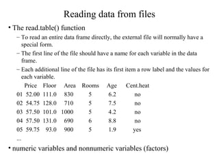
Reading data from files
• HousePrice <- read.table("houses.data", header=TRUE)
Price Floor Area Rooms Age Cent.heat
52.00 111.0 830 5 6.2 no
54.75 128.0 710 5 7.5 no
57.50 101.0 1000 5 4.2 no
57.50 131.0 690 6 8.8 no
59.75 93.0 900 5 1.9 yes
...
• The data file is named ‘input.dat’.
– Suppose the data vectors are of equal length and are to be read in in parallel.
– Suppose that there are three vectors, the first of mode character and the remaining
two of mode numeric.
• The scan() function
– inp<- scan("input.dat", list("",0,0))
– To separate the data items into three separate vectors, use assignments like
label <- inp[[1]]; x <- inp[[2]]; y <- inp[[3]]
– inp <- scan("input.dat", list(id="", x=0, y=0)); inp$id; inp$x; inp$y

Storing data
• Every R object can be stored into and restored from a file with
the commands “save” and “load”.
• This uses the XDR (external data representation) standard of
Sun Microsystems and others, and is portable between MS-
Windows, Unix, Mac.
> save(x, file=“x.Rdata”)
> load(“x.Rdata”)

Importing and exporting data
There are many ways to get data into R and out of R.
Most programs (e.g. Excel), as well as humans, know how to deal
with rectangular tables in the form of tab-delimited text files.
> x = read.delim(“filename.txt”)
also: read.table, read.csv
> write.table(x, file=“x.txt”, sep=“t”)

Importing data: caveats
Type conversions: by default, the read functions try to guess and
autoconvert the data types of the different columns (e.g. number,
factor, character).
 There are options as.is and colClasses to control this – read
the online help
Special characters: the delimiter character (space, comma,
tabulator) and the end-of-line character cannot be part of a data
field.
 To circumvent this, text may be “quoted”.
 However, if this option is used (the default), then the quote
characters themselves cannot be part of a data field. Except if
they themselves are within quotes…
 Understand the conventions your input files use and set the
quote options accordingly.

Statistical models in R
• Regression analysis
– a linear regression model with independent homoscedastic errors
• The analysis of variance (ANOVA)
– Predictors are now all categorical/ qualitative.
– The name Analysis of Variance is used because the original thinking was to
try to partition the overall variance in the response to that due to each of the
factors and the error.
– Predictors are now typically called factors which have some number of
levels.
– The parameters are now often called effects.
– The parameters are considered fixed but unknown —called fixed-effects
models but random-effects models are also used where parameters are taken
to be random variables.

One-Way ANOVA
• The model
–Given a factor α occurring at i =1,…,I levels, with j = 1 ,…,Ji observations
per level. We use the model
–yij = µ+ αi+ εij, i =1,…,I , j = 1 ,…,Ji
• Not all the parameters are identifiable and some restriction is
necessary:
–Set µ=0 and use I different dummy variables.
–Set α1= 0 — this corresponds to treatment contrasts
–Set ΣJiαi= 0 — ensure orthogonality
• Generalized linear models
• Nonlinear regression

Two-Way Anova
• The model yijk = µ+ αi+ βj+ (αβ)ij+ εijk.
– We have two factors, α at I levels and β at J levels.
– Let nij be the number of observations at level i of α and level j of β and let
those observations be yij1, yij2,…. A complete layout has nij≥ 1 for all i, j.
• The interaction effect (αβ)ij is interpreted as that part of the mean
response not attributable to the additiveeffect of αi andβj
.
– For example, you may enjoy strawberries and cream individually, but the
combination is superior.
– In contrast, you may like fish and ice cream but not together.
• As of an investigation of toxic agents, 48 rats were allocated to 3
poisons (I,II,III) and 4 treatments (A,B,C,D).
– The response was survival time in tens of hours. The Data:

Statistical Strategy and Model Uncertainty
• Strategy
– Diagnostics: Checking of assumptions: constant variance, linearity,
normality, outliers, influential points, serial correlation and collinearity.
– Transformation: Transforming the response — Box-Cox, transforming the
predictors — tests and polynomial regression.
– Variable selection: Stepwise and criterion based methods
• Avoid doing too much analysis.
– Remember that fitting the data well is no guarantee of good predictive
performance or that the model is a good representation of the underlying
population.
– Avoid complex models for small datasets.
– Try to obtain new data to validate your proposed model. Some people set
aside some of their existing data for this purpose.
– Use past experience with similar data to guide the choice of model.

Simulation and Regression
• What is the sampling distribution of least squares estimates when
the noises are not normally distributed?
• Assume the noises are independent and identically distributed.
1. Generate ε from the known error distribution.
2. Form y = Xβ + ε.
3. Compute the estimate of β.
• Repeat these three steps many times.
– We can estimate the sampling distribution of using the empirical distribution
of the generated , which we can estimate as accurately as we please by
simply running the simulation for long enough.
– This technique is useful for a theoretical investigation of the properties of a
proposed new estimator. We can see how its performance compares to other
estimators.
– It is of no value for the actual data since we don’t know the true error
distribution and we don’t know β.

Bootstrap
• The bootstrap method mirrors the simulation method but uses
quantities we do know.
– Instead of sampling from the population distribution which we do not know
in practice, we resample from the data itself.
• Difficulty: β is unknown and the distribution of ε is known.
• Solution: β is replaced by its good estimate b and the distribution
of ε is replaced by the residuals e1,…,en.
1. Generate e* by sampling with replacement from e1,…,en.
2. Form y* = X b + e*.
3. Compute b* from (X, y*).
• For small n, it is possible to compute b* for every possible samples
of e1,…,en. 1 n
– In practice, this number of bootstrap samples can be as small as 50 if all we
want is an estimate of the variance of our estimates but needs to be larger if
confidence intervals are wanted.

Implementation
• How do we take a sample of residuals with replacement?
– sample() is good for generating random samples of indices:
– sample(10,rep=T) leads to “7 9 9 2 5 7 4 1 8 9”
• Execute the bootstrap.
– Make a matrix to save the results in and then repeat the bootstrap process
1000 times for a linear regression with five regressors:
bcoef <- matrix(0,1000,6)
–Program: for(i in 1:1000){
newy <- g$fit + g$res[sample(47, rep=T)]
brg <- lm(newy~y)
bcoef[i,] <- brg$coef
}
–Here g is the output from the data with regression
analysis.

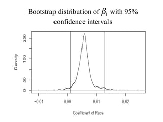
Test and Confidence Interval
• To test the null hypothesis that H0 : β1 = 0 against the alternative
H1 : β1 > 0, we may figure what fraction of the bootstrap sampled
β1 were less than zero:
–length(bcoef[bcoef[,2]<0,2])/1000: It leads to 0.019.
–The p-value is 1.9% and we reject the null at the 5% level.
• We can also make a 95% confidence interval for this parameter by
taking the empirical quantiles:
–quantile(bcoef[,2],c(0.025,0.975))
2.5% 97.5%
0.00099037 0.01292449
• We can get a better picture of the distribution by looking at the
density and marking the confidence interval:
–plot(density(bcoef[,2]),xlab="Coefficient of Race",main="")
–abline(v=quantile(bcoef[,2],c(0.025,0.975)))

Bootstrap distribution of β1 with 95%
confidence intervals

Kernel Density Estimation
• The function `density' computes kernel density estimates with the
given kernel and bandwidth.
– density(x, bw = "nrd0", adjust = 1, kernel = c("gaussian", "epanechnikov",
"rectangular", "triangular", "biweight", "cosine", "optcosine"), window =
kernel, width, give.Rkern = FALSE, n = 512, from, to, cut = 3, na.rm = FALSE)
– n: the number of equally spaced points at which the density is to be
estimated.
• hist(geyser.waiting,freq=FALSE)
lines(density(geyser.waiting))
plot(density(geyser.waiting))
lines(density(geyser.waiting,bw=10))
lines(density(geyser.waiting,bw=1,kernel=“e”))
• Show the kernels in the R parametrization
(kernels <- eval(formals(density)$kernel))
plot (density(0, bw = 1), xlab = "", main="R's density() kernels with bw = 1")
for(i in 2:length(kernels)) lines(density(0, bw = 1, kern = kernels[i]), col = i)
legend(1.5,.4, legend = kernels, col = seq(kernels), lty = 1, cex = .8, y.int = 1)

The Effect of Choice of Kernels
• The average amount of annual precipitation (rainfall) in inches for
each of 70 United States (and Puerto Rico) cities.
• data(precip)
• bw <- bw.SJ(precip) ## sensible automatic choice
• plot(density(precip, bw = bw, n = 2^13), main = "same sd
bandwidths, 7 different kernels")
• for(i in 2:length(kernels)) lines(density(precip, bw = bw, kern =
kernels[i], n = 2^13), col = i)

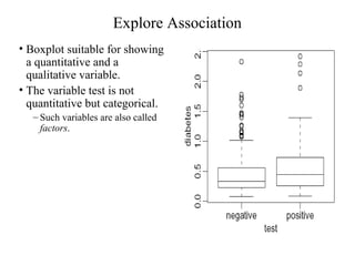
Explore Association
• Data(stackloss)
–It is a data frame with 21 observations on 4 variables.
– [,1] `Air Flow' Flow of cooling air
– [,2] `Water Temp' Cooling Water Inlet Temperature
– [,3] `Acid Conc.' Concentration of acid [per 1000, minus 500]
– [,4] `stack.loss' Stack loss
–The data sets `stack.x', a matrix with the first three
(independent) variables of the data frame, and `stack.loss', the
numeric vector giving the fourth (dependent) variable, are
provided as well.
• Scatterplots, scatterplot matrix:
–plot(stackloss$Ai,stackloss$W)
–plot(stackloss) data(stackloss)
–two quantitative variables.
• summary(lm.stack <- lm(stack.loss ~ stack.x))
• summary(lm.stack <- lm(stack.loss ~ stack.x))

Explore Association
• Boxplot suitable for showing
a quantitative and a
qualitative variable.
• The variable test is not
quantitative but categorical.
– Such variables are also called
factors.

LEAST SQUARES ESTIMATION
• Geometric representation of the estimation β.
– The data vector Y is projected orthogonally onto the model space spanned by
X.
– The fit is represented by projection with the difference between the fit
and the data represented by the residual vector e.
βˆˆ Xy =

Hypothesis tests to compare models
• Given several predictors for a response, we might wonder whether
all are needed.
– Consider a large model, Ω, and a smaller model, ω, which consists of a subset
of the predictors that are in Ω.
– By the principle of Occam’s Razor (also known as the law of parsimony),
we’d prefer to use ω if the data will support it.
– So we’ll take ω to represent the null hypothesis and Ω to represent the
alternative.
– A geometric view of the problem may be seen in the following figure.

Thank You ..
Visit us at..
https://ganeshmkavhar.000webhostapp.com/
https://www.hackerrank.com/ganeshkavhar?hr_r=1

R programming by ganesh kavhar

More Related Content

What's hot

Similar to R programming by ganesh kavhar

More from Savitribai Phule Pune University

Recently uploaded

R programming by ganesh kavhar