This document describes the design and initial results of an L-band radiometer mounted on an unmanned aerial vehicle (UAV) for soil moisture monitoring. The radiometer measures antenna temperature with 1.27K resolution. Software processes the raw data, applying calibration and georeferencing to produce soil moisture maps. Initial field tests show the system can distinguish between soil, water and sun glint reflections. The UAV system provides flexibility and high resolution for applications like precision agriculture compared to spaceborne radiometers.

1. Remote Sensing 2010, 2, 1662-1679; doi:10.3390/rs2071662
OPEN ACCESS
Remote Sensing
ISSN 2072-4292
www.mdpi.com/journal/remotesensing
Article
Design and First Results of an UAV-Borne L-Band Radiometer
for Multiple Monitoring Purposes
Rene Acevo-Herrera 1,*, Albert Aguasca 1, Xavier Bosch-Lluis 1,2, Adriano Camps 1,2,
José Martínez-Fernández 3, Nilda Sánchez-Martín 3 and Carlos Pérez-Gutiérrez 3
1
Remote Sensing Lab, Department of Signal Theory and Communications, Universitat Politècnica
de Catalunya, UPC Campus Nord D3, E-08034 Barcelona, Spain;
E-Mails: rene.acevo@tsc.upc.edu (R.A.-H.); aguasca@tsc.upc.edu (A.A.);
xavier.bosch@tsc.upc.edu (X.B.-L.); camps@tsc.upc.edu (A.C.)
2
IEEC CRAE, UPC, Barcelona, Spain
3
Centro Hispano-Luso de Investigaciones Agrarias (CIALE) Universidad de Salamanca, Parque
Científico Campus de Villamayor C, Río Duero, 12, E-37185 Villamayor (Salamanca), Spain;
E-Mails: jmf@usal.es (J.M.-F.); nilda@usal.es (N.S.-M.); carpegu@usal.es (C.P.-G.)
* Author to whom correspondence should be addressed; E-Mail: rene.acevo@tsc.upc.edu;
Tel.: +34-934-017-362.
Received: 30 April 2010; in revised form: 15 June 2010 / Accepted: 22 June 2010 /
Published: 29 June 2010
Abstract: UAV (unmanned Aerial Vehicle) platforms represent a challenging opportunity
for the deployment of a number of remote sensors. These vehicles are a cost-effective
option in front of manned aerial vehicles (planes and helicopters), are easy to deploy due to
the short runways needed, and they allow users to meet the critical requirements of the
spatial and temporal resolutions imposed by the instruments. L-band radiometers are an
interesting option for obtaining soil moisture maps over local areas with relatively high
spatial resolution for precision agriculture, coastal monitoring, estimation of the risk of
fires, flood prevention, etc. This paper presents the design of a light-weight, airborne
L-band radiometer for deployment in a small UAV, including the hardware and specific
software developed for calibration, geo-referencing, and soil moisture retrieval. First
results and soil moisture retrievals from different field experiments are presented.
Keywords: UAV; airborne sensors; radiometer; soil moisture

2. Remote Sensing 2010, 2 1663
1. Introduction
The interest of the scientific community in the remote measurement of geophysical parameters,
such as the soil moisture (SM) or the sea surface salinity (SSS), has increased in the last years and
much effort has been spent developing research instruments. This has been done mainly by the
European Space Agency (ESA), with the MIRAS/SMOS [1], and the National Aeronautics and Space
Administration (NASA), with AQUARIUS/SAC-D [2,3] and SMAP [4] missions. These space-borne
radiometers have been optimized to measure the aforementioned variables globally, at mesoscale
resolution, with short revisit time (~3 days): pixel size is ~100 km for a 0.1 psu SSS accuracy, or the
pixel size is ~50 km for a 4% SM accuracy. However, these systems are not adequate for regional or
local applications, where higher resolution imagery is required. Airborne microwave radiometers
flying at low altitudes can fulfill this lack of information; they can improve the spatial resolution up to
tens of meters without virtually any revisit time restrictions. Furthermore, these platforms are less
sensitive to atmospheric effects. The SLFMR aboard a Beaver de Havilland [5] and MIRAMAP’s
radiometers [6] are examples of airborne radiometers. In this context, small unmanned aerial vehicles
(UAV) have been found to be the ideal platforms for this kind of remote sensing application [7],
because they are easy to deploy, more flexible, and offer a high level of re-configurability.
This work describes a radiometer system that performs soil moisture mapping from low altitude
small UAV platforms. The paper is organized as follows: Section 2 presents an introductory overview
to the system. Section 3 analyzes the onboard airborne radiometer. The software processor is presented
in Section 4; the processor focuses on radiometer calibration, data geo-referencing and representation,
data interpolation, and SM retrieval algorithms. Section 5 is devoted to the analyses of soil moisture
measurements. Finally, Section 6 summarizes the main conclusions of this paper.
2. System Description
There are a number of restrictions in the design process for a microwave radiometer and the
platform. Assuming their use in precision farming, it is desired to have an absolute accuracy lower
than ≈10 K to determine SM with errors lower than 4%. Additionally, a spatial resolution between 30
and 150 m, while flying at altitudes of up to 300 m, is desirable.
The use of UAV platforms to carry remote sensors imposes not only strong constraints on the size,
weight, and power consumption of the sensors. Moreover, due to the strong vibrations of the UAV
engine induces, an extra effort is required to increase the robustness of the instrument. These vibrations
can reach more than 6 g for gasoline engine powered radio-controlled aircrafts, so that special care
must be taken in the whole system design process.
The main parts of the system that are deployed in the UAV platform are: the L-band Radiometer,
including the antenna, a Global Positioning System (GPS) receiver, an Inertial Motion Unit
(GPS-IMU), and the datalogger. Different UAV platforms have been used, all of them with a 2.5 m
wingspan and 2 m length (Figure 1).These UAVs are able to fly at altitudes of up to 400 m, with cruise
speeds between 25-45 m/s and an endurance of up to 20 min, while carrying a payload of up to 3.5 kg.
The platform is provided with the GPS-IMU for the purpose of geo-referencing the collected
radiometric data. The radiometer’s output signal, the attitude (roll, pitch, and yaw), the altitude, and the

3. Remote Sensing 2010, 2 1664
aircraft speed (vx, vy, and vz) are properly recorded by the onboard data-loggers for later data
processing at a sampling rate of 50 samples per second.
Figure 1. The UAV during a test flight. The ARIEL antenna is located below the fuselage.
3. Airborne L-band Radiometer
A single polarization nadir-looking Dicke radiometer was selected and implemented, due to its
simplicity and sufficient stability when thermally stabilized. The system was designed to require
external periodic calibration only at the beginning and end of each flight (≥20 min).
An important issue to take into account is the antenna. The antenna dimensions of the L-band are
comparable to the size of the UAV itself if a narrow beamwidth is desired (e.g., less than 25° in both
planes). Furthermore, the antenna has to be specifically designed in order to reduce its influence on the
UAV aerodynamics, while preserving the desired performance for radiometric applications. The
designed antenna (Figure 2a) is a flat hexagonal 7-patch array with a 22° beamwidth in both
dimensions [8]. The measured gain, directivity, and radiation ohmic efficiency of this antenna are
15.88 dB, 16.03 dB, and 96.5%, respectively. The effect of the variation of antenna ohmic losses,
which are due to temperature fluctuations, is minimized by incorporating a thermal control attached to
antenna ground plane.
The Airborne RadIomEter at L-band (1.4 GHz) (ARIEL) block diagram is shown in Figure 3. The
heterodyne receiver is divided into three main blocks: the RF front-end, the down-converter, and the
detection block. The RF front-end (1,400 MHz to 1,427 MHz) includes the Dicke switch, which
alternates the detected power between the signal from the antenna and from a matched load. This
signal is properly filtered, amplified, and down-converted to a baseband, where it is detected using a
true rms-detector (output voltage proportional to signal’s standard deviation), followed by a square law
amplifier. Finally, the signal is synchronously demodulated, low-pass filtered, and conditioned before
the analog to digital conversion process.

4. Remote Sensing 2010, 2 1665
Figure 2. (a) Setup for the antenna pattern measurement showing the antenna mounted on
the UAV at the anechoic chamber of the Dept. of Signal Theory and Communications,
Universitat Politècnica de Catalunya [9]. (b) Measured full radiation pattern. (c) Simulated
and measured copolar radiation pattern at the E-plane. Simulation only considered ideal
isotropic radiation elements, and thus, slight differences between simulated and measured
results can be distinguished. (d) Measured cross-polar radiation pattern for the E-plane.
(a) (b)
(c) (d)
Figure 3. ARIEL block diagram.

5. Remote Sensing 2010, 2 1666
The radiometric sensitivity ΔT for a balanced Dicke radiometer is [10]:
2(TREF + TREC )
∆T = , (1)
Bτ
where TREF = 315 K is the physical temperature of the reference load, TREC ≈ 790 K is the receiver’s
noise temperature, B ≈ 30 MHz is the system’s noise bandwidth, and τ is the integration time.
The maximum integration time is determined by the minimum dwell time according to,
FPmin BW × hmin
= , (2)
vmax vmax
where FPmin is the smallest footprint, BW is the antenna beamwidth, hmin is the minimum flight height,
and vmax is the maximum flight speed. With these parameters, the theoretical radiometric resolution is
ΔT = 1.27 K for an integration time of τ = 100 ms.
The radiometer was implemented using commercial “off-the-shelf” components. The radiometer
front-end was integrated in a 100 × 60 × 15 mm monoblock box (Figure 4). The total weight, including
the batteries, the antenna, and its radome, is less than 3 kg. If the thermal control of the radiometer is
included, the total power consumption of the system is less than 10 W, which facilitates the use of light
weight Lithium Polymer batteries as the main power supply.
Figure 4. ARIEL RF front end 100 × 60 × 20 mm compared to the size of a 1 euro coin.
4. ARIEL Soil Moisture Retrieval Processor
A specific software processor for soil moisture retrieval has been developed to obtain soil moisture
maps from the radiometric measurements. The input data files (GPS, IMU, attitude, and raw
radiometric data) are selected from a specific graphical user interface (GUI), where the radiometric
calibration procedure is defined. This radiometric data calibration procedure is performed before, after,
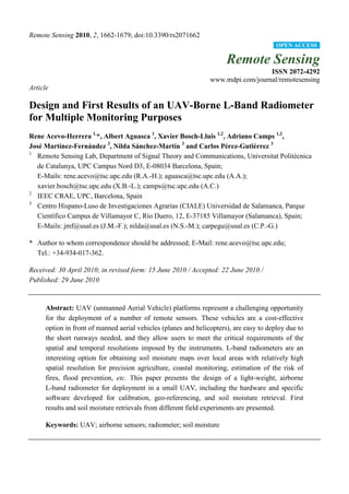
or before and after the flight, according to an established protocol. Figure 5a shows this calibration
process. The calibration is based on the selection of the intervals in the raw data where the hot or cold
loads were measured.
Two independent dataloggers were used, one for the GPS, and the other for the inertial and
radiometric data. To synchronize their data, cross-correlation techniques were used that applied the
altitude information from GPS and the barometer (Figure 5b).

6. Remote Sensing 2010, 2 1667
Figure 5. Data processing (a) Calibration of radiometer output (selection of calibration
intervals), (b) Synchronization of the altitude data from GPS data and the barometric
information data synchronization.
(a)
(b)
As shown in Figure 6a, histograms can also be plotted to detect relevant information, such as
intervals of interest, and by extracting the desired ranges of antenna temperatures or aircraft height.
Interesting parameters to be displayed are the antenna temperature and soil moisture maps in time
intervals. The flight trajectory can be illustrated together with the corresponding antenna footprints
plotted along the ground track (Figure 6b). The processor includes attitude and altitude filters to limit
the range of valid incidence angles, eliminate Sun glints at high banking angles, radio frequency
interference (RFI) peaks, or potential recording errors of the dataloggers.

7. Remote Sensing 2010, 2 1668
Figure 6. Images showing the kind of target present in the scene. Test performed in a
coastal zone. (a) Histogram plot in which different targets and other signals could be
distinguished during the measurement: soil, water, calibration, and sun glints. (b)
Trajectory plot of the flight superimposed with brightness temperatures.
(a) (b)
Finally, in order to fully cover a specific area (typically 1 km × 1 km) with the UAV flying at low
altitudes (under 300 m), the flight plan is designed in such a way that several overpasses at different
heights (i.e., with different spatial resolutions) are obtained. In order to merge all the collected
information, each footprint has to be properly weighted with the antenna’s radiation pattern. Therefore,
interpolation techniques have been developed to obtain images with soil moisture or antenna
temperature information (Section 4.1.3). These images are then geo-referenced and linked to a map
using Keyhole-Mark-up-Language (KML) [11] files that can be superimposed on Google Earth maps
for a better interpretation.
4.1. Algorithm Description and Procedures
The soil moisture retrieval algorithm proceeds as follows:
• Raw data resampling.
• Radiometric calibration.
• Ground projection of the antenna footprint, taking into account the attitude and position of the
platform.
• Spatial interpolation.
• Soil moisture retrieval.
The algorithm is described step by step in the following sections.
4.1.1. Data Resampling
GPS’ largest errors are in the vertical direction. A barometric sensor is used to correct this
information, and to refer all heights to ground level, so as to properly compute the antenna footprints.
In order to geo-reference the radiometric data, it is necessary to synchronize the barometric altimeter,
the GPS, and the radiometric data, since they are acquired at different sampling frequencies and by

8. Remote Sensing 2010, 2 1669
different dataloggers. The altitude is referenced to the ground’s altitude in order to properly compute
the antenna footprints.
4.1.2. Radiometric Calibration
The radiometer’s raw-data are converted into antenna temperatures through the radiometric
calibration. In a Dicke radiometer, the relationship between its output voltage, vo, and the antenna
temperature can be expressed as [10]:
vo = a (TREF − TA ) + b (3)
where TREF is the temperature of the reference load (measured with a thermometer), TA is the antenna
temperature, and a and b are gain and offset constants to be determined during the absolute calibration
with the hot-cold method [12]. A thermally isolated microwave absorber placed just in front of the
antenna is used as a hot load, and pointing the antenna to the sky gives the equivalent of a cold load.
In case of temperature drifts during the flight, a linear behavior between two hot or cold load
calibrations performed just before and after the flight, is assumed. In this case, the calibrations
parameters can be determined as follows:
a f − ab
a (t ) = a b + (t − tb ) (4a)
t f − tb
and
b f − bb
b(t ) = bb + (t − tb ) (4b)
t f − tb
where t is the time and the subscripts b and f mean before and after the flight.
Finally, the time dependent coefficients a(t) and b(t) are used with TREF to compute the calibrated
antenna temperature at each sample. In case of the failure of all calibrations, a laboratory calibration
with constant coefficients measured in the anechoic chamber can be used. For an integration time of
τ = 100 ms, the measured calibration standards have standard deviations of σ hot = 0.0045 V and
σ cold = 0.0052 V, which translate into sensitivities of ΔThot = 0.84 K and ΔTcold = 1.22 K; these values
are in agreement with theoretical predictions (Section 3).
4.1.3. Data Merging and Spatial Interpolation
Once the flight trajectory has been determined, the ground projection is performed and the footprint
size and shape are determined. Then, the radiometric data has to be properly processed in order to
obtain a geocoded SM map that can be linked to a KML file; to be finally overlaid with Google Earth
maps. As described before, the data sampling rate is f s = 50 Hz, and the UAV speed is vUAV ≈ 40 m s .
This means that the aircraft has moved 0.8 m between consecutive samples. If an average footprint of
100 m is considered, the pixels have a high-level of overlap, and thus, data must be
properly interpolated.
For geo-statistical applications, the Kriging method [13] provides the optimal interpolator. It
assigns weights according to a data-driven weighting function (spatial covariance values obtained
through a semivariogram). However, for simplicity and computational speed considerations, the

9. Remote Sensing 2010, 2 1670
algorithm performs an alternative method of assigning a weight to each footprint according to the
modified two-dimensional (bivariate) Gaussian density function (GDF) that best fits the antenna
pattern mainlobe. Each GDF has been adjusted to ensure that for the 3dB antenna footprint contour,
the GDF value falls to the half of the maximum (−3 dB in antenna terms).
Finally, the resulting pixel is the product of a merge of all values from the footprints that intersect a
given pixel. Every temperature value of the pixel is obtained from a weighted average of the different
looks:
n
∑ GDF (d k k )·Z k
ˆ
Zi = k =1
,
n (5)
∑ GDF (d
k =1
k k )
ˆ
where Zk is the value of the kth contributing antenna footprint, Z i is the estimated value for the pixel ith,
dk is the distance from the center of the pixel to the center of the kth contributing antenna footprint,
GDFk is the GDF of the kth contributing antenna footprint, and n is the total number of
contributing footprints.
In this procedure, the footprints generated at lower altitudes will have a higher influence on the
obtained pixel. In addition, to ensure nadir look observations, only footprints with incidence angles
lower or equal to 10° are computed in the process. This will be further explained in the
following section.
4.2. Soil Moisture Retrieval
The brightness temperature of the surface is measured by an antenna far away. In this case, the
apparent temperature, TAP, is the key parameter that depends on the brightness temperature of the
surface under observation (TB), the atmospheric upward radiation (TUP), the atmospheric downward
radiation scattered and reflected by the surface (TSC), and the atmospheric attenuation (La). The
downward radiation is mainly generated by the cosmic radiation level of the sky T≈ 2.7 K at L -band,
and the downwelling atmospheric contribution, TDNatm ≈ 2.1 K, at zenith. These values are fairly
constant and will not affect the quality of the measurement, and are thus usually ignored. Since TUP ≈ 0
at low altitudes, TSC is much smaller than the required accuracy and La ≈ 1 (for θ = 0° ), at low
altitudes, the apparent temperature TAP at L-band can be approximated by the temperature emitted by
the surface (TB) weighted by the antenna pattern.
1 2
=TA
Ωp ∫∫ T (θ , φ ) F (θ , φ )
4π
AP n dΩ , (6)
where Fn (θ ,φ ) is the normalized antenna voltage pattern, Ωp is the equivalent antenna beam solid
angle, and θ is the incidence angle.
The brightness temperature TB of a soil covered by vegetation is usually estimated as the
contribution of three terms: (i) the radiation from the soil that is attenuated by the overlying vegetation,
(ii) the upward radiation from the vegetation, and (iii) the downward radiation from the vegetation,
reflected by the soil, and attenuated by the canopy [12]:

10. Remote Sensing 2010, 2 1671
 1 − ebs   1  ebs
 (1 − ω ) Tveg +
model
TBp = 1 +  1 − Tsoil , (7)
 
Lveg   
Lveg  Lveg

where ebs= (1 − Γ ) is the bare soil emissivity, Г is the reflection coefficient, p is the polarization, Tveg
p
and Tsoil are the physical temperatures of the vegetation and soil, respectively, = exp(τ ⋅ sec θ )
Lveg
[Np] is the attenuation due to the vegetation cover, τ = b × VWC is the optical thickness, b [m2/kg] is a
vegetation dependent factor [14], VWC is the vegetation water content [kg/m2], and ω is the single
scattering albedo. This formulation is known as the τ-ω model [14] and is based on the single
scattering approach proposed in [15].
In the case of bare soil: τ = 0, Lveg ≈ 1, and ω = 0 and (7) reduces to
TBp (θ )= (1 − Γ (θ ) ) T
p
soil (8)
where the reflection coefficient at the air-ground interface Γ p (θ ) is computed using the Wang
model [16] as:
Γ p (θ= (1 − Qs ) ⋅ Γ spec , p (θ ) + Qs ⋅ Γ spec ,q (θ )  ⋅ exp ( −hs cosn θ ) ,
)   (9)
where Qs is the mixing polarization parameter, and hs is the surface roughness. Both are functions of
the frequency. Recent studies have shown that hs also depends on soil moisture [17]. In order to
retrieve soil moisture from the antenna temperature at a single direction, some assumptions are made:
• The soil is bare and smooth (surface roughness parameter hs = 0).
• Only incidence angles smaller than 10° have been retained, since the angular dependence of TB
around 0° is weak.
To determine the impact of the incidence angle, the emissivity of a bare flat soil is plotted versus
soil moisture for three different incidence angles (θ = 0°, 10°, and 30°; Figure 7a). It could be seen that
for incidence angles of up to 10°, the error is smaller than 1% compared with a 0° incidence. For
incidence angles up to 30°, the error rises to 6%. In Figure 7b, the impact of vegetation cover is
illustrated, showing the emissivity of soil versus SM for two different kinds of soils: bare soil and
wheat. Compared with a bare soil, the error is 6% for 22 cm height vegetation and 15% for 60 cm
vegetation. These values are obtained with an incidence angle of θ = 0°.
In order to speed up the retrieval process, an emissivity look-up table has been created with SM
entries. The scattered radiation is also included for average soil moisture conditions [12]. Then, for a
given Tph and TA, the SM is readily estimated.

11. Remote Sensing 2010, 2 1672
Figure 7. Emissivity as a function of SM for (a) a bare flat soil versus SM at three
different angles (θ = 0°, 10°, and 30°). The error compared with a θ = 0° is: 1% at θ =10°,
and 6% at θ =30°, (b) for two different kind of soils: bare soil and pasture. The error is: 6%
for 22 cm height vegetation and 15% for 60 cm height vegetation at θ = 0°.
(a) (b)
Emissivity as a function of soil moisture for different incident angles Emissivity as a function of soil moisture for different soil types
0.95 0.95
0º Bare soil
0.9 10º 22 cm vegetation
0.9
30º 61 cm vegetation
0.85
0.85
0.8
0.8
Emissivity
Emissivity
0.75
0.75
0.7
0.7
0.65
0.65
0.6
0.55 0.6
0.5 0.55
0 5 10 15 20 25 30 35 40 0 5 10 15 20 25 30 35 40
SM(%) SM(%)
5. Experimental Results
Three experimental field campaigns have been conducted over different scenarios to retrieve soil
moisture maps. The selected scenarios were:
(1) Ripollet site surroundings (Barcelona, Spain), used for agricultural applications: land and crop
monitoring, with different irrigation levels,
(2) Ebro River mouth (Deltebre, Spain), not presented in this work, used for agricultural (rice
fields) and coastal applications [18], and
(3) REMEDHUS site (Salamanca, Spain), used for SMOS calibration and validation (CAL/VAL)
activities [19].
5.1. Soil Moisture Measurements at Ripollet Site Surroundings
The Ripollet site surroundings were chosen because the region has a radio control model flying club
near agricultural fields. These fields showed interesting changes in soil moisture during the first half of
2009 due to the different irrigation levels during winter and spring. A measured soil moisture map
from the Ripollet field is displayed in Figure 8a. The flight corresponds to April 29 (day of year (DoY)
= 119), 2009. In situ ground truth measurements were taken with a moisture sensor ECH2O EC-5 [20]
at a vertical depth of 5 cm. Measurements were performed and two samples averaged. The positions of
the soil moisture measurements were geo-coded using a commercial GPS receiver. The soil moisture
ground truth (SM-GT) map was spatially interpolated with the same pixel resolution of the retrieved
SM map and is shown in Figure 8b.

12. Remote Sensing 2010, 2 1673
Figure 8. Experimental results of the Ripollet site surroundings, April 29 (DoY=119),
2009. Google Earth image size 1.5 km × 1 km. (a) Soil moisture map of Ripollet
agricultural fields. (b) Ground truth soil moisture map of Ripollet.
(a) (b)
Figure 9 shows an error map of the retrieved soil moisture with ARIEL versus the ground truth
measurements. In the upper left part of the error image, the absolute value varies from 6% to 9%. In
this zone there is a hill with a 10% slope covered by dense wheat fields. In the center of the image, the
error reaches 1%. There are two noticeable regions (shown in red) where the error reaches up to 16%.
One region corresponds to the aircraft runway made of concrete, and the other is covered by tall
vegetation (3 m height cane).
Figure 9. Retrieved soil moisture error map with ARIEL compared to ground truth
measurements. In the center of the image, the absolute error reaches 1% and rises up to 9%
in the upper left (data cursor value is 8.27%). Two noticeable zones (red and yellow),
where the error reaches up to 16%, are the runway and a tall vegetation area (3 m
height cane).
5.2. Soil Moisture Retrieval Tests at the Remedhus, SMOS Cal/Val Site Zamora, Spain
GRAJO (GPS and Radiometric Joint Observations) is a joint initiative between UPC and the Centro
Hispano Luso de Investigaciones Agrarias (CIALE)/Universidad de Salamanca (USAL). The CIALE

13. Remote Sensing 2010, 2 1674
group is in charge of the in situ measurements using TDR and Hydra Probes automatic sensors [21] in
order to obtain, simultaneously, soil moisture and temperature at 5, 25, and 50 cm depths. UPC is in
charge of the radiometric and the GPS reflectometer data acquisitions.
The GRAJO field campaigns in support to the SMOS calibration or validation have been carried out
in Vadillo de la Guareña, Zamora, Spain from November 2008 until May 2010 [19].
The objectives of GRAJO are threefold:
• To validate and calibrate the SMOS-derived soil moisture map, at SMOS pixel-size levels.
• To study the variability of soil moisture within the SMOS footprint.
• To test pixel disaggregation techniques development in order to improve the spatial resolution of
SMOS observations. These algorithms have been tested using airborne radiometric
measurements over REMEDHUS acquired with the ARIEL radiometer.
The experiment with ARIEL at the REMEDHUS test site was planned to be performed over this
very heterogeneous area, where the measured SM has variations from 2 to 50% in a 2 km2 area. These
conditions allowed one to validate the SM retrieval algorithm over those different kinds of terrains and
SM values. The method’s feasibility could be tested thanks to the information from a ground-truth SM
map provided by CIALE.
Figure 10 shows a land use map of the area where four kinds of soil can be distinguished: cereal,
vineyard, human-made buildings, and rangeland. There are also rural ways, trees, and a creek. This
kind of land use implies a high degree of variability of the SM with abrupt changes.
Figure 10. Land use map for the experiment in Vadillo de la Guareña (Zamora, Spain).
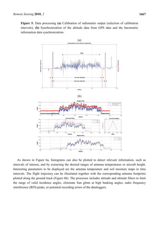
Flight measurements were carried out in the morning right after sunrise and in the evening right
before sunset in order to reduce the effect of Sun interferences (due to reflections over the terrain). The
retrieved soil moisture maps from the two flights are plotted in Figure 11a. Figure 11b shows the soil
moisture ground truth map obtained by the CIALE/USAL team, which has been generated using
Kriging interpolation techniques. The ground truth maps show variations in SM from 2% to
almost 50%.

14. Remote Sensing 2010, 2 1675
Figure 11. Experimental measurements in Vadillo de la Guareña (Zamora, Spain), March
25 (DoY = 84), 2009. (a) Soil moisture map mixing two different flights (square area of
2.28 km2). Flight 1 covers the right image part and flight 2, the left one. (b) Ground-truth
soil moisture map provided by CIALE/USAL.
(a) (b)
Since the experiment was carried out in a very heterogeneous area, the most homogeneous zones
with lower variations in the SM (up to 15%) are analyzed first. Figure 12a shows the error map
between the retrieved SM map from flight 1 (Figure 11a) and the ground truth measurements
(Figure 11b) of part of the scenario (center of Figure 11a). The ground truth showed a variation of SM
from 25 to 40%, and the obtained error map (difference between retrieved SM and ground truth in %)
goes from 1 to 6%. The same results are obtained in other parts of the scenario. Figure 12b shows the
error map of the left part of the scenario with information retrieved from second flight. The same
results are obtained in this flight.
Figure 12. Error maps for the homogeneous zone from the retrieved SM versus ground
truth measurements of (a) flight 1, and (b) flight 2.
(a) (b)
Error map Error map
0.1 0.1
41.3068
0.09 0.09
41.3054
41.3066 0.08 0.08
41.3052
0.07 0.07
41.3064
0.06 0.06
41.305
41.3062
0.05 0.05
41.3048
41.306 0.04 0.04
0.03 41.3046 0.03
41.3058
0.02 0.02
41.3056 41.3044
0.01 0.01
0 0
-5.3692 -5.369 -5.3688 -5.3686 -5.3684 -5.3682 -5.3755 -5.375 -5.3745 -5.374
Figure 13a shows the error map in the complete image. It is easy to see that this absolute error
increases at the corners of the area from 12% up to 20% due to the substantial reduction in the number
of overpasses. It must be pointed out that some areas showed variations in SM from 4% to 46% at

15. Remote Sensing 2010, 2 1676
distances closer than 70 m. These areas have been interpolated by the radiometer if a footprint of 100
m is observed that implies a large error in the retrieved SM value.
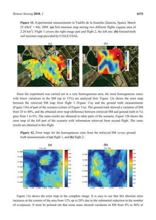
Figure 13b represents the error map in the complete image from the second flight. There are two
zones in the center of the image where the error reaches 20%, for which some considerations must be
taken into account. The flight was performed in the afternoon, and the ground truth map was taken in
the morning simultaneously with the first flight so that in this zone, the variability in SM is higher due
to the drying. One limitation of generating ground truth maps with interpolation methods is the
variability of SM values in short distances. A source of error in the ground truth information is that of
the accuracy of the sensor, which in this case is 1.5% [21].
Figure 13. Error maps for the full areas from retrieved SM versus ground truth
measurements of (a) flight 1, and (b) flight 2. The dark blue points show the locations of
the ground truth measurements.
(a) (b)
Error map
41.3085 0.2
41.308 0.18
41.3075 0.16
41.307 0.14
41.3065 0.12
41.306 0.1
41.3055 0.08
41.305 0.06
41.3045 0.04
41.304 0.02
0
-5.372 -5.371 -5.37 -5.369 -5.368 -5.367
To better understand these large differences, biophysical parameters of the vegetation present in the
site are provided in Table 1. The VWC was determined during the measurement, and the normalized
difference vegetation index (NDVI) was measured with a USB4000 miniature fiber optic spectrometer
from ocean optics.
Table 1. Biophysical parameters of the vegetation present in Vadillo de la Guareña
(Zamora, Spain), March 25 (DoY = 84), 2009.
NDVI Growing Cycle VWC (%) FVC (%)
Grass/Pasture 0.60 to 0.85 Development 66 to 78 55 to 75
Barley/Cereal 0.63 to 0.72 Development 70 to 75 49 to 61
Vineyard −0.01 to 0 Dormancy -- --
Unproductive −0.05 to 0 -- -- --
Based on Table 1 information, and on the land use map of Figure 10, the best results in the first
flight were obtained over unproductive areas (bare soil or poor vegetation). The average errors were
obtained over grass or pasture zones where higher vegetation indices were present.

16. Remote Sensing 2010, 2 1677
The largest errors are obtained in the vineyard area. Despite its low vegetation index and poor water
content, this area has a particular orography, with a 10% slope and a road (without ground truth
information) that separates a very dense grass zone from the vineyard. Furthermore, this part of the
scenario was not well covered during the flight; thus, few footprints contributed to the pixels.
In the second flight, the biggest errors are present over cereal zones where a high vegetation index
is present. The same performance occurs over the roads where it is not possible to have ground
truth information.
Other noticeable artifact in the image of Figure 11a is an apparent circular feature of the SM
retrieved maps. It occurs in the zones where few over flights were performed, which means that few
samples contribute to the pixel generation and the antenna footprint is depicted.
6. Conclusions
This work has presented the design and development of an airborne light weight radiometer at
L-band (ARIEL). It also presents the software processor that includes different calibration techniques
and interpolation and merging techniques. These techniques allow immediate processing of the data
just at the end of the flight.
The flexibility of the UAV system has been applied for soil moisture mapping in cereal and
vineyard fields located in the REMEDHUS SMOS CAL/VAL site. Results show that geo-referenced
Google Earth maps of soil moisture and brightness temperature maps were obtained with estimated
absolute errors between 1% and 6%. These results were obtained at homogeneous zones in
agricultural fields.
The experimental tests planned in heterogeneous and vegetation covered soils show large errors
where abrupt changes in SM are present and Krigging interpolation is prone to larger errors. The best
results are obtained over more homogeneous zones, and the best image quality is achieved over the
zones in which more overflights were performed.
Some improvements on the system are planned in order to increase the resolution. Also, a unique
GPS-IMU unit will be included to avoid data resampling.
Acknowledgements
This project has been supported by the projects: MIDAS-5 ESP2007-65667-C04-02 and AYA
2008-05906-C02-01/ESP, TEC 2005.
This project has been supported by a grant of Universitat Politècnica de Catalunya, UPC Pre-PhD
Scholarships.
This work, conducted as part of the award “Passive Advanced Unit (PAU): A Hybrid L-band
Radiometer, GNSS-Reflectometer and IR-Radiometer for Passive Remote Sensing of the Ocean” made
under the European Heads of Research Councils and European Science Foundation EURYI (European
Young Investigator) Awards scheme in 2004, was supported by funds from the Participating
Organizations of EURYI and the EC Sixth Framework Program.

17. Remote Sensing 2010, 2 1678
References
1. Kerr, Y.H.; Waldteufel, P.; Wigneron, J.; Martinuzzi, J.; Font, J.; Berger, M. Soil moisture
retrieval from space: the Soil Moisture and Ocean Salinity (SMOS) mission. IEEE Trans. Geosci.
Remote Sens. 2001, 39, 1729-1735.
2. Lagerloef, G.; LeVine, D.; Chao, Y.; Colomb, R. Aquarius/SAC-D Mission; A key to
understanding the links between salinity and climate variability. OS43C-02; AGU-ASLO Ocean
Sciences, OS43C-02, February 2005.
3. Le Vine, D.M.; Lagerloef, G.S.E.; Colomb, F.R.; Yueh, S.H.; Pellerano, F.A. Aquarius: An
instrument to monitor sea surface salinity from space. IEEE Trans. Geosci. Remote Sens. 2007,
45, 2040-2050.
4. Committee on Earth Science and Applications from Space: A Community Assessment and
Strategy for the Future, National Research Council. Earth Science and Applications from Space:
National Imperatives for the Next Decade and Beyond, 2007. Available online:
http://www.nap.edu (accessed on 12 May 2010).
5. Miller, J.L.; Goodberlet, M.A.; Zaitzeff, J.B. Airborne salinity mapper makes debut in coastal
zone. Trans. American Geophysical Union EOS 1998, 79, 173-177.
6. Haarbrink, R.; Shutko, A. New airborne sensor for soil moisture mapping. In Proceedings of the
Second International Workshop on The Future of Remote Sensing, ISPRS Inter-Commission WG
I/V, Autonomous Navigation, VITO/ISPRS, Antwerp, Belgium, October 2006.
7. McIntyre, E.M.; Gasiewski, A.J.; Leuski, V. Development of a lobe-differencing correlation
radiometer (LDCR) for airborne UAV SSS mapping. In Proceedings of the IEEE International
Geoscience and Remote Sensing Symposium 2007, Barcelona, Spain, 2007; pp. 1095-1097.
8. Valencia, E.; Acevo, R.; Bosch-Lluis, X.; Aguasca, A.; Rodriguez-Alvarez, N.; Ramos-Perez, I.;
Marchan-Hernandez, J.F.; Glenat, M.; Bou, F.; Camps, A. initial results of an airborne
light-weight l-band radiometer. In Proceedings of the IEEE International Geoscience and Remote
Sensing Symposium 2008, Boston, MA, USA, 2008; pp. II-1176-II-1179.
9. Remote sensing laboratory. Available online: http://www.tsc.upc.edu/rslab/index.php (accessed
on 12 May 2010).
10. Skou, N.; Le Vine, D. Microwave Radiometer Systems Design and Analysis, 2nd ed.; Artech
House, Inc.: Norwood, MA, USA, 2006; p. 222.
11. KML standard. Available online: http://www.opengeospatial.org/standards/kml/ (accessed on 12
May 2010).
12. Ulaby, FT.; Moore, R.K.; Fung, A.K. Microwave Remote Sensing. Active and Passive Vol I.
Fundamentals and Radiometry, 1st ed.; Artech House: Norwood, MA, USA, 1981; p. 456.
13. Stein, A.; Van der Meer, F.; Gorte, B. Spatial Statistics for Remote Sensing: Remote Sensing and
Digital Image Processing; Kluwer Academic Publishers: Dordrecht, The Netherlands, 1999;
p. 300.
14. Van de Griend, A.A.; Wigneron, J. The b-factor as a function of frequency and canopy type at
h-polarization. IEEE Trans. Geosci. Remote Sens. 2004, 42, 786-794.
15. Kirdiashev, K.P.; Chukhlantsev, A.A.; Shutko, A.M. Microwave radiation of the earth’s surface in
the presence of vegetation cover. Radio Eng. Electron. Phys. 1979, 2, 37-56.

18. Remote Sensing 2010, 2 1679
16. Wang, J.R.; Schmugge, T.J. An empirical model for the complex dielectric permittivity of soils as
a function of water content. IEEE Trans. Geosci. Remote Sens. 1980, 18, 288-296.
17. Escorihuela, M.J.; Kerr, Y.H.; de Rosnay, P.; Wigneron, J.; Calvet, J.; Lemaitre, F. A simple
model of the bare soil microwave emission at l-band. IEEE Trans. Geosci. Remote Sens. 2007, 45,
1978-1987.
18. Acevo-Herrera, R.; Aguasca, A.; Bosch-Lluis, X.; Camps, A. On the Use of Compact L-band
Dicke Radiometer (ARIEL) and UAV for Soil Moisture and Salinity Map Retrieval: 2008/2009
Field Experiments. In Proceedings of the IEEE International Geoscience and Remote Sensing
Symposium 2009, Cape Town, South Africa, 2009; pp. IV729-IV732.
19. Monerris, A.; Rodriguez-Alvarez, N.; Vall-llossera, M.; Camps, A.; Piles, M.; Martinez-
Fernandez, J.; Sanchez-Martin, N.; Perez-Gutierrez, C.; Baroncini-Turricchia, G.; Acevo, R.;
Aguasca, A. The GPS and RAdiometric Joint Observations Experiment at the REMEDHUS Site
(Zamora-Salamanca Region, Spain). In Proceedings of the IEEE International Geoscience and
Remote Sensing Symposium 2009, Cape Town, South Africa, 2009; pp. III286-III289.
20. ECH2O Soil Moisture Sensor. Available online: http://www.decagon.com/ag_research/
soil/ec5.php (accessed on 12 May 2010).
21. Stevens’ Hydra Probe II Soil Moisture Sensor (SDI-12 / RS485). Available online:
http://www.stevenswater.com/catalog/products/soil_sensors/datasheet/hydraprobeiidatasheetnew
web.pdf (accessed on 12 May 2010).
© 2010 by the authors; licensee MDPI, Basel, Switzerland. This article is an Open Access article
distributed under the terms and conditions of the Creative Commons Attribution license
(http://creativecommons.org/licenses/by/3.0/).

19. Copyright of Remote Sensing is the property of MDPI Publishing and its content may not be copied or emailed
to multiple sites or posted to a listserv without the copyright holder's express written permission. However,
users may print, download, or email articles for individual use.