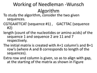
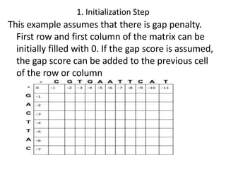
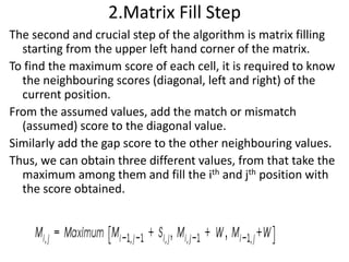
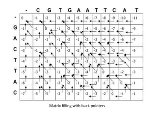
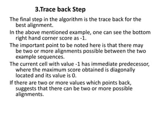
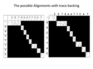
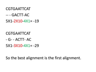
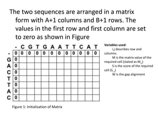
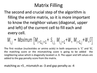
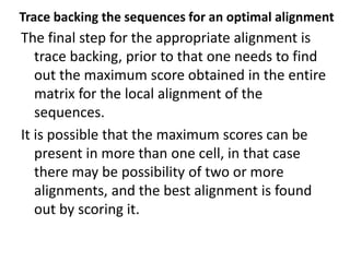
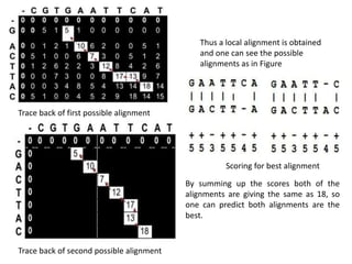
The document discusses global and local sequence alignment algorithms. It explains that global alignment algorithms align sequences from start to end by adding gaps, while local alignment finds regions of highest similarity. The Needleman-Wunsch algorithm performs global alignment using dynamic programming to find the best end-to-end match. The Smith-Waterman algorithm performs local alignment using dynamic programming to find the best local matches between sequences. Both algorithms initialize a scoring matrix and fill it using neighboring cell scores to trace back the highest scoring alignments.

1. Global and Local Alignment
Algorithms
Computer applications for
Biosciences and Bioinformatics
Module III b

2. Pairwise alignment via Dynamic
Programming
Dynamic programming is a method by which a
larger problem may be solved by first solving
smaller, partial versions of the problem.
 Global alignment algorithms start at the
beginning of two sequences and add gaps to
each until the end of one is reached.
 Local alignment algorithms finds the region
(or regions) of highest similarity between two
sequences and build the alignment outward
from there.

3. Global Alignment
This is generally known as the Needleman-Wunsch
algorithm, after the first paper in the field of
computational molecular biology to apply dynamic
programming to the global alignment problem.
[Needleman, S.B. & Wunsch, C.D. (1970) “A general
method applicable to the search for similarities in
the amino acid sequences of two proteins.” J. Mol.
Biol. 48:443-453.]
The Needleman-Wunsch algorithm creates a global
alignment over the length of both sequences

4. • Closely related sequences which are of same
length are very much appropriate for global
alignment. Here, the alignment is carried out
from beginning till end of the sequence to find
out the best possible alignment.

5. Global algorithms are often not effective for
highly diverged sequences - do not reflect the
biological reality that two sequences may only
share limited regions of conserved sequence.
Sometimes two sequences may be derived from
ancient recombination events where only a
single functional domain is shared.
Global methods are useful when you want to
force two sequences to align over their entire
length

6. Local alignment
Smith & Waterman proposed simply that a local
alignment of two sequences allow arbitrary-
length segments of each sequence to be aligned,
with no penalty for the unaligned portions of the
sequences. Otherwise, the score for a local
alignment is calculated the same way as that for a
global alignment.
[Smith, T.F. & Waterman, M.S. (1981)
“Identification of common molecular
subsequences.” J. Mol. Biol. 147:195-197.]

7. Sequences which are suspected to have
similarity or even dissimilar sequences can be
compared with local alignment method. It
finds local regions with high level of similarity.

8. Useful for comparing protein sequences that
share a common motif (conserved pattern) or
domain (independently folded unit) but differ
elsewhere
Useful for comparing DNA sequences that share
a similar motif but differ elsewhere
Useful for comparing protein sequences against
genomic DNA sequences (long stretches of
uncharacterized sequence)
More sensitive when comparing highly diverged
sequences

10. Global Alignment
Two closely related sequences:
Needleman & Wunsch algorithm creates an end-to-end alignment.
Two sequences sharing several regions of local similarity

11. Working of Needleman -Wunsch
Algorithm
To study the algorithm, consider the two given
sequences.
CGTGAATTCAT (sequence #1) , GACTTAC (sequence
#2)
length (count of the nucleotides or amino acids) of the
sequence 1 and sequence 2 are 11 and 7
respectively.
The initial matrix is created with A+1 column’s and B+1
row’s (where A and B corresponds to length of the
sequences).
Extra row and column is given, so as to align with gap,
at the starting of the matrix as shown in Figure

12. The simple basic scoring schema can be assumed as, if two residues (nucleotide or
amino acid) at ith and jth position are same, matching score is 1 (S(i,j)= 1) or if
the two residues at ith and jth position are not same, mismatch score is assumed
as -1 (S(i,j)= -1 ). The gap score(w) or gap penalty is assumed as -1 .
The dynamic programming matrix is defined with three different steps.
1.Initialization of the matrix with the scores possible.
2.Matrix filling with maximum scores.
3.Trace back the residues for appropriate alignment.
Variables used:
i,j describes row and columns.
M is the matrix value of the required cell
(stated as Mi,j)
S is the score of the required cell (Si, j)
W is the gap alignment

13. 1. Initialization Step
This example assumes that there is gap penalty.
First row and first column of the matrix can be
initially filled with 0. If the gap score is assumed,
the gap score can be added to the previous cell
of the row or column

14. 2.Matrix Fill Step
The second and crucial step of the algorithm is matrix filling
starting from the upper left hand corner of the matrix.
To find the maximum score of each cell, it is required to know
the neighbouring scores (diagonal, left and right) of the
current position.
From the assumed values, add the match or mismatch
(assumed) score to the diagonal value.
Similarly add the gap score to the other neighbouring values.
Thus, we can obtain three different values, from that take the
maximum among them and fill the ith and jth position with
the score obtained.

15. Matrix filling with back pointers

16. The final step in the algorithm is the trace back for the
best alignment.
In the above mentioned example, one can see the bottom
right hand corner score as -1.
The important point to be noted here is that there may
be two or more alignments possible between the two
example sequences.
The current cell with value -1 has immediate predecessor,
where the maximum score obtained is diagonally
located and its value is 0.
If there are two or more values which points back,
suggests that there can be two or more possible
alignments.
3.Trace back Step

17. By continuing the trace back step by the above
defined method, one would reach to the 0th
row, 0th column.
Following the above described steps, alignment
of two sample sequences can be found.
The best alignment among the alignments can
be identified by using the maximum alignment
score

18. The possible Alignments with trace backing

19. CGTGAATTCAT
-- - GACTT-AC
5X1-2X10-4X1= -19
CGTGAATTCAT
- G- - ACTT- AC
5X1-3X10-4X1= -29
So the best alignment is the first alignment.

20. Working of Smith-Waterman Algorithm
Intialization of Matrix
The basic steps for the algorithm are similar to that of
Needleman-Wunsch algorithm.
The steps are:
1. Initialization of a matrix.
2. Matrix Filling with the appropriate scores.
3. Trace back the sequences for a suitable alignment.
To study the Local sequence alignment consider the
given below sequences.
CGTGAATTCAT (sequence#1 or A)
GACTTAC (sequence #2 or B)

21. The two sequences are arranged in a matrix
form with A+1 columns and B+1 rows. The
values in the first row and first column are set
to zero as shown in Figure
Figure 1: Initialization of Matrix
Variables used:
i,j describes row and
columns.
M is the matrix value of the
required cell (stated as Mi,j)
S is the score of the required
cell (Si, j)
W is the gap alignment

22. Matrix Filling
The second and crucial step of the algorithm is
filling the entire matrix, so it is more important
to know the neighbor values (diagonal, upper
and left) of the current cell to fill each and
every cell.
The first residue (nucleotides or amino acids) in both sequences is ‘C’ and ‘G’,
the matching score or the mismatching score is going to be added the
neighboring value which is diagonally located i.e. 0. The upper and left values are
added to the gap penalty score from the matrix.
matching as +5 , mismatch as -3 and gap penalty as -4

23. Figure 2: Matrix filling with back pointers

24. Trace backing the sequences for an optimal alignment
The final step for the appropriate alignment is
trace backing, prior to that one needs to find
out the maximum score obtained in the entire
matrix for the local alignment of the
sequences.
It is possible that the maximum scores can be
present in more than one cell, in that case
there may be possibility of two or more
alignments, and the best alignment is found
out by scoring it.

25. In this example we can see the maximum score
in the matrix as 18, which is found in two
positions that lead to multiple alignments, so
the best alignment has to be found.
So the trace back begins from the position which
has the highest value, pointing back with the
pointers, thus find out the possible
predecessor, then move to next predecessor
and continue until we reach the score 0

26. Trace back of first possible alignment
Trace back of second possible alignment
Thus a local alignment is obtained
and one can see the possible
alignments as in Figure
Scoring for best alignment
By summing up the scores both of the
alignments are giving the same as 18, so
one can predict both alignments are the
best.