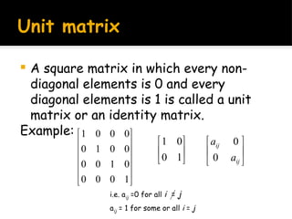
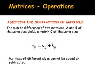
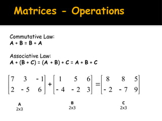
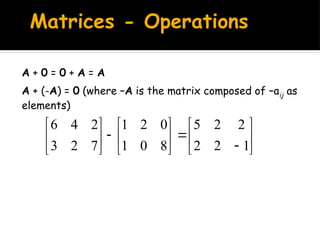
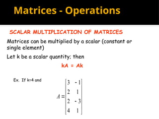
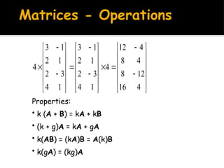
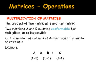
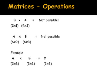
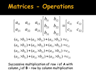
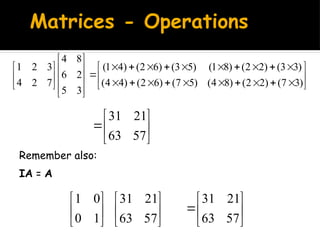
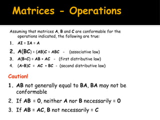
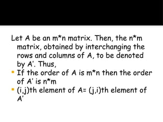
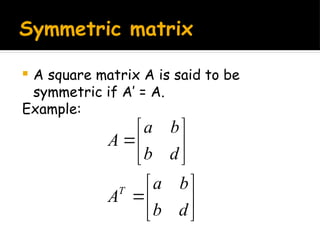
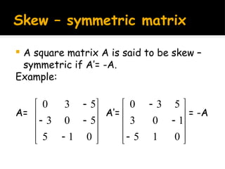
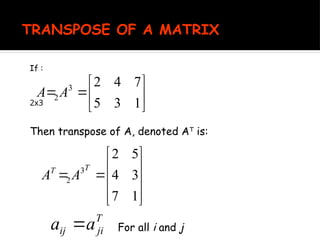
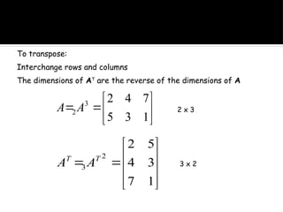
The document provides a comprehensive overview of matrices, covering their definitions, types (such as row, column, zero, square, diagonal, unit, and equal matrices), and various operations including addition, subtraction, scalar multiplication, and multiplication of matrices. It explains advanced concepts such as transpose, symmetric, and skew-symmetric matrices, along with their properties and relevant mathematical laws. Additionally, it includes references for further reading.

1. Matrices
Hafiz NADEEM (ACCA)
BBA,SCM,ADP
(1st
semester)
Imperial College of
Business Studies

2. Topics to be covered
 Definition
 How to describe matrices ?
 Types of matrices
 Operation in matrices
 Transpose of matrices
 References

3. Definition
 Matrices is a set or group of numbers
arrange in a square or rectangular
array enclose by two brackets.
 Matrices can be written as an m*n
matrix.
 ‘m’ is horizontal lines called rows.
 ‘n’ is vertical line called columns.

4. How to describe matrix
 An element occurring in the ith row and
jth column of a matrix A will be called
the (i , j)th element of A to be denoted
by aij














mn
ij
m
m
n
ij
in
ij
a
a
a
a
a
a
a
a
a
a
a
a
2
1
2
22
21
12
11
...
...




Amxn=

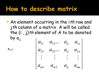
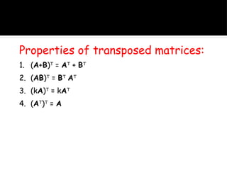
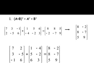
5. e.g. matrix [A] with elements aij
Amxn=














mn
ij
m
m
n
ij
in
ij
a
a
a
a
a
a
a
a
a
a
a
a
2
1
2
22
21
12
11
...
...





6. TYPE OF
MATRICES

7.  Row matrix
 Column matrix
 Zero or null matrix
 Square matrix
 Diagonal matrix
 Scalar matrix
 Unit matrix
 Comparable matrix
 Equal matrix

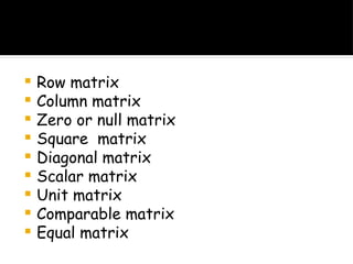
8. Row matrix
A matrix having only one row is known as
a row matrix or a row vector.
Example:
• A= [5 18] is a row matrix of order 1x2.
• B= [ 2 4 3 7] is a row matrix of order
1x4.

9. Column matrix
 A matrix having only one column is
known as column matrix or a column
vector.
Example:










2
4
1






 3
1












1
21
11
m
a
a
a


10. Zero or Null matrix
 A matrix each of whose elements is
zero is called a zero is called zero or
null matrix.
Example:










0
0
0










0
0
0
0
0
0
0
0
0
0

ij
a For all i,j

11. Square matrix
 A matrix having the same number of
rows and column is called a square
matrix.
Example:






0
3
1
1










1
6
6
0
9
9
1
1
1

12. Diagonal matrix
 A square matrix in which every non-
diagonal element is zero is called a
diagonal matrix.
Example:










1
0
0
0
2
0
0
0
1












9
0
0
0
0
5
0
0
0
0
3
0
0
0
0
3
i.e. aij =0 for all i = j
aij = 0 for some or all i = j

13. Unit matrix
 A square matrix in which every non-
diagonal elements is 0 and every
diagonal elements is 1 is called a unit
matrix or an identity matrix.
Example:












1
0
0
0
0
1
0
0
0
0
1
0
0
0
0
1






1
0
0
1
i.e. aij =0 for all i = j
aij = 1 for some or all i = j






ij
ij
a
a
0
0

14. Operations in
matrices

15. Matrices - Operations
ADDITION AND SUBTRACTION OF MATRICES
The sum or difference of two matrices, A and B of
the same size yields a matrix C of the same size
ij
ij
ij b
a
c 

Matrices of different sizes cannot be added or
subtracted

16. Matrices - Operations
Commutative Law:
A + B = B + A
Associative Law:
A + (B + C) = (A + B) + C = A + B + C


























9
7
2
5
8
8
3
2
4
6
5
1
6
5
2
1
3
7
A
2x3
B
2x3
C
2x3

17. Matrices - Operations
A + 0 = 0 + A = A
A + (-A) = 0 (where –A is the matrix composed of –aij as
elements)





















1
2
2
2
2
5
8
0
1
0
2
1
7
2
3
2
4
6

18. Matrices - Operations
SCALAR MULTIPLICATION OF MATRICES
Matrices can be multiplied by a scalar (constant or
single element)
Let k be a scalar quantity; then
kA = Ak
Ex. If k=4 and















1
4
3
2
1
2
1
3
A

19. Matrices - Operations














































4
16
12
8
4
8
4
12
4
1
4
3
2
1
2
1
3
1
4
3
2
1
2
1
3
4
Properties:
• k (A + B) = kA + kB
• (k + g)A = kA + gA
• k(AB) = (kA)B = A(k)B
• k(gA) = (kg)A

20. Matrices - Operations
MULTIPLICATION OF MATRICES
The product of two matrices is another matrix
Two matrices A and B must be conformable for
multiplication to be possible
i.e. the number of columns of A must equal the number
of rows of B
Example.
A x B = C
(1x3) (3x1) (1x1)

21. Matrices - Operations
B x A = Not possible!
(2x1) (4x2)
A x B = Not possible!
(6x2) (6x3)
Example
A x B = C
(2x3) (3x2) (2x2)

22. Matrices - Operations























22
21
12
11
32
31
22
21
12
11
23
22
21
13
12
11
c
c
c
c
b
b
b
b
b
b
a
a
a
a
a
a
22
32
23
22
22
12
21
21
31
23
21
22
11
21
12
32
13
22
12
12
11
11
31
13
21
12
11
11
)
(
)
(
)
(
)
(
)
(
)
(
)
(
)
(
)
(
)
(
)
(
)
(
c
b
a
b
a
b
a
c
b
a
b
a
b
a
c
b
a
b
a
b
a
c
b
a
b
a
b
a
























Successive multiplication of row i of A with
column j of B – row by column multiplication

23. Matrices - Operations











































)
3
7
(
)
2
2
(
)
8
4
(
)
5
7
(
)
6
2
(
)
4
4
(
)
3
3
(
)
2
2
(
)
8
1
(
)
5
3
(
)
6
2
(
)
4
1
(
3
5
2
6
8
4
7
2
4
3
2
1







57
63
21
31
Remember also:
IA = A






1
0
0
1






57
63
21
31







57
63
21
31

24. Matrices - Operations
Assuming that matrices A, B and C are conformable for the
operations indicated, the following are true:
1. AI = IA = A
2. A(BC) = (AB)C = ABC - (associative law)
3. A(B+C) = AB + AC - (first distributive law)
4. (A+B)C = AC + BC - (second distributive law)
Caution!
1. AB not generally equal to BA, BA may not be
conformable
2. If AB = 0, neither A nor B necessarily = 0
3. If AB = AC, B not necessarily = C

25. Transpose of
matrices

26. Let A be an m*n matrix. Then, the n*m
matrix, obtained by interchanging the
rows and columns of A, to be denoted
by A’. Thus,
 If the order of A is m*n then the order
of A’ is n*m
 (i,j)th element of A= (j,i)th element of
A’

27. Symmetric matrix
 A square matrix A is said to be
symmetric if A’ = A.
Example:














d
b
b
a
A
d
b
b
a
A
T

28. Skew – symmetric matrix
 A square matrix A is said to be skew –
symmetric if A’= -A.
Example:
A= A’= = -A














0
1
5
5
0
3
5
3
0













0
1
5
1
0
3
5
3
0

29. TRANSPOSE OF A MATRIX
If :








1
3
5
7
4
2
3
2 A
A
2x3












1
7
3
4
5
2
3
2
T
T
A
A
Then transpose of A, denoted AT
is:
T
ji
ij a
a  For all i and j

30. To transpose:
Interchange rows and columns
The dimensions of AT
are the reverse of the dimensions of A








1
3
5
7
4
2
3
2 A
A












1
7
3
4
5
2
2
3
T
T
A
A
2 x 3
3 x 2

31. Properties of transposed matrices:
1. (A+B)T
= AT
+ BT
2. (AB)T
= BT
AT
3. (kA)T
= kAT
4. (AT
)T
= A

32. 1. (A+B)T
= AT
+ BT


























9
7
2
5
8
8
3
2
4
6
5
1
6
5
2
1
3
7












9
5
7
8
2
8






































9
5
7
8
2
8
3
6
2
5
4
1
6
1
5
3
2
7

33. (AB)T
= BT
AT
 
   
8
2
3
0
2
1
0
1
2
1
1
8
2
8
2
2
1
1
3
2
0
0
1
1




































34. References
 Aggarwal, R.S. (2005). “Mathematics”,
Eighth edition, pp. 3-13, Bharati Bhawan
Publications.
 Vasistha, A.R. (2014). “Matrices”, pp.
20-32, Krishna Publication.
 Gupta, S.C. (2009). “Fundamental of
Mathematics” pp. 36-42, Sutanchand &
Sons Publication.

35. Thank You