Downloaded 29 times


![> 3 + 7
[1] 10
> sqrt(100) + 3 ^ 2
[1] 19
> 1:10
[1] 1 2 3 4 5 6 7 8 9 10
> (1:10) ^ 2
[1] 1 4 9 16 25 36 49 64 81 100
Tuesday, 16 February 2010](https://image.slidesharecdn.com/11-simulation-100216095912-phpapp01/85/11-Simulation-13-320.jpg)
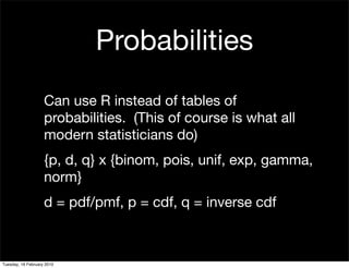
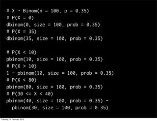
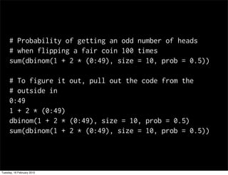
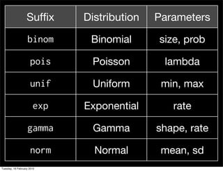
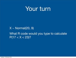

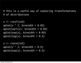

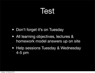
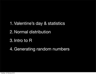
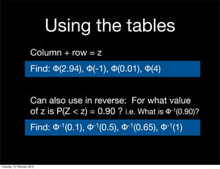
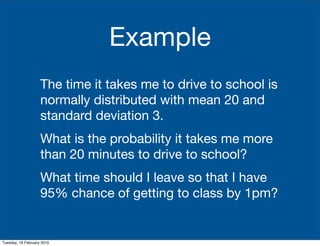
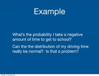
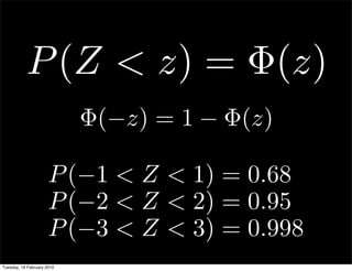
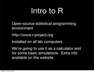
This document contains notes from a statistics course. It discusses upcoming tests and help sessions. It also outlines topics to be covered, including the normal distribution, introduction to R, generating random numbers, and working with probabilities and distributions in R. Examples are provided on calculating probabilities and generating random values from distributions in R.


![Introduction to Signal Processing Orfanidis [Solution Manual]](https://cdn.slidesharecdn.com/ss_thumbnails/51628783-solution-signal-processing-160422182740-thumbnail.jpg?width=640&height=640&fit=bounds)


![Week7 Quiz Help 2009[1]](https://cdn.slidesharecdn.com/ss_thumbnails/week7quizhelp20091-091012152329-phpapp02-thumbnail.jpg?width=640&height=640&fit=bounds)


