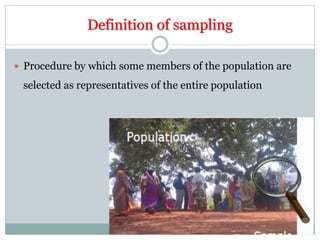
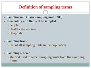
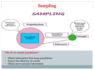
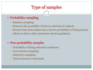
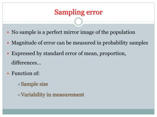
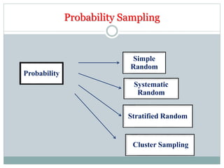
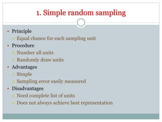
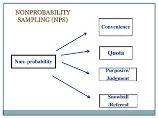
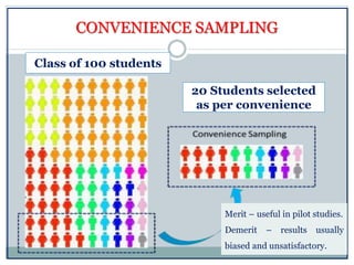
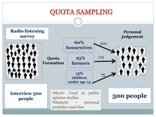
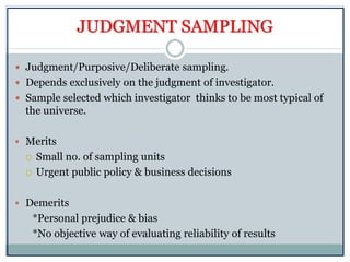
Definition of sampling
 Procedure by which some members of the population are
selected as representatives of the entire population
Study population
 The study population is the population to which the results
of the study will be inferred
The study population depends upon the research question:
How many injections do people received each year in India?
 Study population: Population of India
How many needle-sticks health care workers experience each
year in India?
 Study population: Health care workers of India
Sample
The sample needs to be representative of the population in
terms of
1. Time:
Seasonality
Day of the week
Time of the day
2. Place:
Urban
Rural
3. Persons
Age
Sex
Other demographic characteristics
Definition of sampling terms
 Sampling unit (Basic sampling unit, BSU)
 Elementary unit that will be sampled
 People
 Health care workers
 Hospitals
 Sampling frame
 List of all sampling units in the population
 Sampling scheme
 Method used to select sampling units from the sampling
frame
Sampling
Why do we sample populations?
• Obtain information from large populations
• Ensure the efficiency of a study
• Obtain more accurate information
Example
 The Ministry of Health of a country X wants to estimate the
proportion of children in elementary schools who have
been immunized against childhood infectious diseases
 The task must be completed in one month
 The objective is to estimate the proportion of immunized
children
Type of samples
 Probability sampling
 Random sampling
 Removes the possibility of bias in selection of subjects
 Ensures that each subject has a known probability of being chosen
 Allows to draw valid conclusions about population
 Non-probability samples
 Probability of being selected is unknown
 Convenience sampling
 Subjective sampling
 Time/resources constraints
Sampling error
 No sample is a perfect mirror image of the population
 Magnitude of error can be measured in probability samples
 Expressed by standard error of mean, proportion,
differences…
 Function of:
Sample size
Variability in measurement
Simple
Random
Systematic
Random
Stratified Random
Cluster Sampling
Probability
Probability Sampling
1. Simple random sampling
 Principle
 Equal chance for each sampling unit
 Procedure
 Number all units
 Randomly draw units
 Advantages
 Simple
 Sampling error easily measured
 Disadvantages
 Need complete list of units
 Does not always achieve best representation
2. Systematic sampling
 Principle
 A unit drawn every k units
 Equal chance of being drawn for each unit
 Procedure
 Calculate sampling interval (k = N/n)
 Draw a random number (≤ k) for starting
 Draw every k units from first unit
 Advantages
 Ensures representativity across list
 Easy to implement
 Disadvantage
 Dangerous if list has cycles
Example of systematic sampling
Every eighth house is selected
3. Stratified sampling
 Principle
 Classify population into homogeneous subgroups (strata)
 Draw sample in each strata
 Combine results of all strata
 Advantage
 More precise if variable associated with strata
 All subgroups represented, allowing separate conclusions
about each of them
 Disadvantages
 Sampling error difficult to measure
 Loss of precision if small numbers sampled in individual strata
Example of stratified sampling
 Estimate vaccination coverage in a country
 One sample drawn in each region
 Estimates calculated for each stratum
 Each strata weighted to obtain estimate for country
4. Cluster sampling
 Principle
 Random sample of groups (“clusters”) of units
 All or proportion of units included selected clusters
 Advantages
 Simple: No list of units required
 Less travel/resources required
 Disadvantages
 Imprecise if clusters homogeneous (Large design effect)
 Sampling error difficult to measure
Cluster sampling
 The sampling unit is not a subject, but a group (cluster) of
subjects.
 It is assumed that:
 The variability among clusters is minimal
 The variability within each cluster is what is observed in the
general population
The two stages of a cluster sample
1.First stage: Probability proportional to size
 Select the number of clusters to be included
 Compute a cumulative list of the populations in each unit with a
grand total
 Divide the grand total by the number of clusters and obtain the
sampling interval
 Choose a random number and identify the first cluster
 Add the sampling interval and identify the second cluster
 By repeating the same procedure, identify all the clusters
2.Second stage
 In each cluster select a random sample using a sampling frame of
subjects (e.g. residents) or households
• In cluster sampling, the clusters are the primary sampling
unit (PSU’s) .
• Units within the clusters are the secondary sampling units
(SSU’s)
CLUSTER SAMPLING
Non- probability
Convenience
Quota
Purposive/
Judgment
Snowball
/Referral
NONPROBABILITY
SAMPLING (NPS)
CONVENIENCE SAMPLING
Class of 100 students
20 Students selected
as per convenience
Merit – useful in pilot studies.
Demerit – results usually
biased and unsatisfactory.
Quota
Formation
Interview 500
people
Personal
judgement
Radio listening
survey
60%
housewives
25%
farmers
15%
children
under age 15
300
125
75
500 people
QUOTA SAMPLING
Merit- Used in public
opinion studies
Demerit – personal
prejudice and bias
JUDGMENT SAMPLING
 Judgment/Purposive/Deliberate sampling.
 Depends exclusively on the judgment of investigator.
 Sample selected which investigator thinks to be most typical of
the universe.
 Merits
 Small no. of sampling units
 Urgent public policy & business decisions
 Demerits
*Personal prejudice & bias
*No objective way of evaluating reliability of results
JUDGMENT SAMPLING - EXAMPLE
CLASS OF 20
STUDENTS
Sample size for a
study= 8
JUDGMENT
SAMPLE OF 8
STUDENTS
SNOWBALL SAMPLING
 Used when the desired sample characteristic is rare
 When locating respondents is extremely difficult or cost
prohibitive.
 Snowball sampling relies on referrals from initial subjects to
generate additional subjects
 Merit
 For difficult to reach populations (other methods may not yield
any results).
 Demerit
 not representative of the population and will result in a biased
sample as it is self-selecting.
SNOWBALL SAMPLING - STEPS
 Make contact with one or two cases in the population.
 Ask these cases to identify further cases.
 Ask these new cases to identify further new cases.
 Stop when either no new cases are given or the sample is as large
as is manageable.
Key issues
 We cannot study the whole population so we sample it
 Taking a sample leads to sampling error, which is measurable
 Good design and quality assurance ensure validity and while
appropriate sample size will ensure precision
 Probability samples are the only one that allow use of statistics as
we know them
Types of Data
 Qualitative
 Nominal
Eg. Color of Eyes
 Ordinal
Eg. Stages of disease condition
 Quantitative
 Discrete
Eg. Family size
 Continuous
Eg. Height / Weight
Describe –Central Value
 Data is not information.
 Summarize
 Average
 Mean
 Median
 Mode
Arithmetic Mean (AM)
 Most commonly used; Simply called MEAN
 Add all the observed values(Sum=∑Xi)
 Mean =Sum / n
 Sample Mean is denoted by x̅
 Population Mean is denoted by μ
Example
 Age of 10 Pregnant women
 26, 31, 25, 21, 26, 26, 27, 25, 27, and 26
 Sum= (26+31+25+21+26+26+27+25+27+26) = 260
 n = 10
 Mean = sum / n= 260/10 = 26 years
Median
 The Median describes literally the middle value of the
distribution
 Divides the distribution exactly into two halves (i.e. 50% of
the data will fall on either side)
 Useful when there are extreme values
Example
 Duration (days) of hospital stay of 11 patients
 1, 2, 3, 4, 5, 6, 7, 8, 8, 9, 77 (Arranged in ascending order)
 Median is the middle value (6thvalue) = 6
 (Mean = 11.8)
 If n is even; then take average of middle two values.
Mode
 The Mode is the value that occurs most frequently
 Mode is the only location statistics to be used –for nominal
data -not measurable characteristic
 Epidemiology –Describing an epidemic with respect to
TIME
Example
 •Colour preference of people for their car
 Mode = Yellow
Colour preference No. of persons
Green 354
Yellow 852
White 310
Red 474
Describe –Dispersion
 Is it enough to know the average?
 Example of swimming pool.
 •Measures of variability
 Range
 Inter-quartile range
 Mean deviation from mean
 Variance / Standard deviation
RANGE
Definition:
 The difference between the Minimum and the Maximum value of
the observations
Advantage:
 A quick and easy indicator of dispersion.
Disadvantage:
 Influenced by extreme values; Uses only two data points
INTER-QUARTILE RANGE
Definition:
 Defined as the interval between the value of the upper quartile
(Q3) and the lower quartile (Q1)
 Inter Quartile Range = Q3–Q1
Advantage:
 Unaffected by the extreme values
Disadvantage:
 Covers only the middle 50% observations
INTER QUARTILE RANGE
 The range of a data is divided into four (25%)
MEAN DEVIATION
 Definition: The mean deviation is the average of the absolute
(ignoring the sign) deviations of the observations from the
arithmetic mean.
 Advantage: It is based on all the observations in the group. It is
easy to grasp the meaning of the procedure.
 Disadvantage: It ignores the sign of the difference of the value of
the observation and arithmetic mean.
 It is not widely used because of the availability of a more
advantageous measure.
STANDARD DEVIATION -SD (σ)
 Definition: The SD is the square root of the average of the squared
deviations of the observations from the arithmetic mean
 The square of the SD is called variance
 Advantage: The SD is the most important measure of distribution.
While the variance is in unit squared, the SD is expressed in the same
units of measurement as the observation. It is suitable for further
analysis
 The SD together with arithmetic mean is useful for description of the
data
Normal Distribution Curve
Coefficient of Variation (CV)
 Purpose: To compare the relative variability in different groups
 Definition: The coefficient of variation is the SD expressed as a
percentage of the arithmetic mean (AM).

 CV = SD x 100
AM
Summary
 Choose appropriate central / dispersion value
 Mean / SD –if no extreme values
 Median / IQR –if there are extreme values
 Mode /Range –for qualitative variables/ time distribution
in epidemic curve
 Mean and SD are used the most.
2.7.21 sampling methods data analysis

2.7.21 sampling methods data analysis

  • 3.
    Definition of sampling Procedure by which some members of the population are selected as representatives of the entire population
  • 4.
    Study population  Thestudy population is the population to which the results of the study will be inferred The study population depends upon the research question: How many injections do people received each year in India?  Study population: Population of India How many needle-sticks health care workers experience each year in India?  Study population: Health care workers of India
  • 5.
    Sample The sample needsto be representative of the population in terms of 1. Time: Seasonality Day of the week Time of the day 2. Place: Urban Rural 3. Persons Age Sex Other demographic characteristics
  • 6.
    Definition of samplingterms  Sampling unit (Basic sampling unit, BSU)  Elementary unit that will be sampled  People  Health care workers  Hospitals  Sampling frame  List of all sampling units in the population  Sampling scheme  Method used to select sampling units from the sampling frame
  • 7.
    Sampling Why do wesample populations? • Obtain information from large populations • Ensure the efficiency of a study • Obtain more accurate information
  • 8.
    Example  The Ministryof Health of a country X wants to estimate the proportion of children in elementary schools who have been immunized against childhood infectious diseases  The task must be completed in one month  The objective is to estimate the proportion of immunized children
  • 9.
    Type of samples Probability sampling  Random sampling  Removes the possibility of bias in selection of subjects  Ensures that each subject has a known probability of being chosen  Allows to draw valid conclusions about population  Non-probability samples  Probability of being selected is unknown  Convenience sampling  Subjective sampling  Time/resources constraints
  • 10.
    Sampling error  Nosample is a perfect mirror image of the population  Magnitude of error can be measured in probability samples  Expressed by standard error of mean, proportion, differences…  Function of: Sample size Variability in measurement
  • 11.
  • 12.
    1. Simple randomsampling  Principle  Equal chance for each sampling unit  Procedure  Number all units  Randomly draw units  Advantages  Simple  Sampling error easily measured  Disadvantages  Need complete list of units  Does not always achieve best representation
  • 13.
    2. Systematic sampling Principle  A unit drawn every k units  Equal chance of being drawn for each unit  Procedure  Calculate sampling interval (k = N/n)  Draw a random number (≤ k) for starting  Draw every k units from first unit  Advantages  Ensures representativity across list  Easy to implement  Disadvantage  Dangerous if list has cycles
  • 14.
    Example of systematicsampling Every eighth house is selected
  • 15.
    3. Stratified sampling Principle  Classify population into homogeneous subgroups (strata)  Draw sample in each strata  Combine results of all strata  Advantage  More precise if variable associated with strata  All subgroups represented, allowing separate conclusions about each of them  Disadvantages  Sampling error difficult to measure  Loss of precision if small numbers sampled in individual strata
  • 16.
    Example of stratifiedsampling  Estimate vaccination coverage in a country  One sample drawn in each region  Estimates calculated for each stratum  Each strata weighted to obtain estimate for country
  • 17.
    4. Cluster sampling Principle  Random sample of groups (“clusters”) of units  All or proportion of units included selected clusters  Advantages  Simple: No list of units required  Less travel/resources required  Disadvantages  Imprecise if clusters homogeneous (Large design effect)  Sampling error difficult to measure
  • 18.
    Cluster sampling  Thesampling unit is not a subject, but a group (cluster) of subjects.  It is assumed that:  The variability among clusters is minimal  The variability within each cluster is what is observed in the general population
  • 19.
    The two stagesof a cluster sample 1.First stage: Probability proportional to size  Select the number of clusters to be included  Compute a cumulative list of the populations in each unit with a grand total  Divide the grand total by the number of clusters and obtain the sampling interval  Choose a random number and identify the first cluster  Add the sampling interval and identify the second cluster  By repeating the same procedure, identify all the clusters 2.Second stage  In each cluster select a random sample using a sampling frame of subjects (e.g. residents) or households
  • 20.
    • In clustersampling, the clusters are the primary sampling unit (PSU’s) . • Units within the clusters are the secondary sampling units (SSU’s) CLUSTER SAMPLING
  • 21.
  • 22.
    CONVENIENCE SAMPLING Class of100 students 20 Students selected as per convenience Merit – useful in pilot studies. Demerit – results usually biased and unsatisfactory.
  • 23.
    Quota Formation Interview 500 people Personal judgement Radio listening survey 60% housewives 25% farmers 15% children underage 15 300 125 75 500 people QUOTA SAMPLING Merit- Used in public opinion studies Demerit – personal prejudice and bias
  • 24.
    JUDGMENT SAMPLING  Judgment/Purposive/Deliberatesampling.  Depends exclusively on the judgment of investigator.  Sample selected which investigator thinks to be most typical of the universe.  Merits  Small no. of sampling units  Urgent public policy & business decisions  Demerits *Personal prejudice & bias *No objective way of evaluating reliability of results
  • 25.
    JUDGMENT SAMPLING -EXAMPLE CLASS OF 20 STUDENTS Sample size for a study= 8 JUDGMENT SAMPLE OF 8 STUDENTS
  • 26.
    SNOWBALL SAMPLING  Usedwhen the desired sample characteristic is rare  When locating respondents is extremely difficult or cost prohibitive.  Snowball sampling relies on referrals from initial subjects to generate additional subjects  Merit  For difficult to reach populations (other methods may not yield any results).  Demerit  not representative of the population and will result in a biased sample as it is self-selecting.
  • 27.
    SNOWBALL SAMPLING -STEPS  Make contact with one or two cases in the population.  Ask these cases to identify further cases.  Ask these new cases to identify further new cases.  Stop when either no new cases are given or the sample is as large as is manageable.
  • 28.
    Key issues  Wecannot study the whole population so we sample it  Taking a sample leads to sampling error, which is measurable  Good design and quality assurance ensure validity and while appropriate sample size will ensure precision  Probability samples are the only one that allow use of statistics as we know them
  • 30.
    Types of Data Qualitative  Nominal Eg. Color of Eyes  Ordinal Eg. Stages of disease condition  Quantitative  Discrete Eg. Family size  Continuous Eg. Height / Weight
  • 31.
    Describe –Central Value Data is not information.  Summarize  Average  Mean  Median  Mode
  • 32.
    Arithmetic Mean (AM) Most commonly used; Simply called MEAN  Add all the observed values(Sum=∑Xi)  Mean =Sum / n  Sample Mean is denoted by x̅  Population Mean is denoted by μ
  • 33.
    Example  Age of10 Pregnant women  26, 31, 25, 21, 26, 26, 27, 25, 27, and 26  Sum= (26+31+25+21+26+26+27+25+27+26) = 260  n = 10  Mean = sum / n= 260/10 = 26 years
  • 34.
    Median  The Mediandescribes literally the middle value of the distribution  Divides the distribution exactly into two halves (i.e. 50% of the data will fall on either side)  Useful when there are extreme values
  • 35.
    Example  Duration (days)of hospital stay of 11 patients  1, 2, 3, 4, 5, 6, 7, 8, 8, 9, 77 (Arranged in ascending order)  Median is the middle value (6thvalue) = 6  (Mean = 11.8)  If n is even; then take average of middle two values.
  • 36.
    Mode  The Modeis the value that occurs most frequently  Mode is the only location statistics to be used –for nominal data -not measurable characteristic  Epidemiology –Describing an epidemic with respect to TIME
  • 37.
    Example  •Colour preferenceof people for their car  Mode = Yellow Colour preference No. of persons Green 354 Yellow 852 White 310 Red 474
  • 38.
    Describe –Dispersion  Isit enough to know the average?  Example of swimming pool.  •Measures of variability  Range  Inter-quartile range  Mean deviation from mean  Variance / Standard deviation
  • 39.
    RANGE Definition:  The differencebetween the Minimum and the Maximum value of the observations Advantage:  A quick and easy indicator of dispersion. Disadvantage:  Influenced by extreme values; Uses only two data points
  • 40.
    INTER-QUARTILE RANGE Definition:  Definedas the interval between the value of the upper quartile (Q3) and the lower quartile (Q1)  Inter Quartile Range = Q3–Q1 Advantage:  Unaffected by the extreme values Disadvantage:  Covers only the middle 50% observations
  • 41.
    INTER QUARTILE RANGE The range of a data is divided into four (25%)
  • 42.
    MEAN DEVIATION  Definition:The mean deviation is the average of the absolute (ignoring the sign) deviations of the observations from the arithmetic mean.  Advantage: It is based on all the observations in the group. It is easy to grasp the meaning of the procedure.  Disadvantage: It ignores the sign of the difference of the value of the observation and arithmetic mean.  It is not widely used because of the availability of a more advantageous measure.
  • 43.
    STANDARD DEVIATION -SD(σ)  Definition: The SD is the square root of the average of the squared deviations of the observations from the arithmetic mean  The square of the SD is called variance  Advantage: The SD is the most important measure of distribution. While the variance is in unit squared, the SD is expressed in the same units of measurement as the observation. It is suitable for further analysis  The SD together with arithmetic mean is useful for description of the data
  • 44.
  • 45.
    Coefficient of Variation(CV)  Purpose: To compare the relative variability in different groups  Definition: The coefficient of variation is the SD expressed as a percentage of the arithmetic mean (AM).   CV = SD x 100 AM
  • 46.
    Summary  Choose appropriatecentral / dispersion value  Mean / SD –if no extreme values  Median / IQR –if there are extreme values  Mode /Range –for qualitative variables/ time distribution in epidemic curve  Mean and SD are used the most.