Download as PDF, PPTX


![In a more formal way
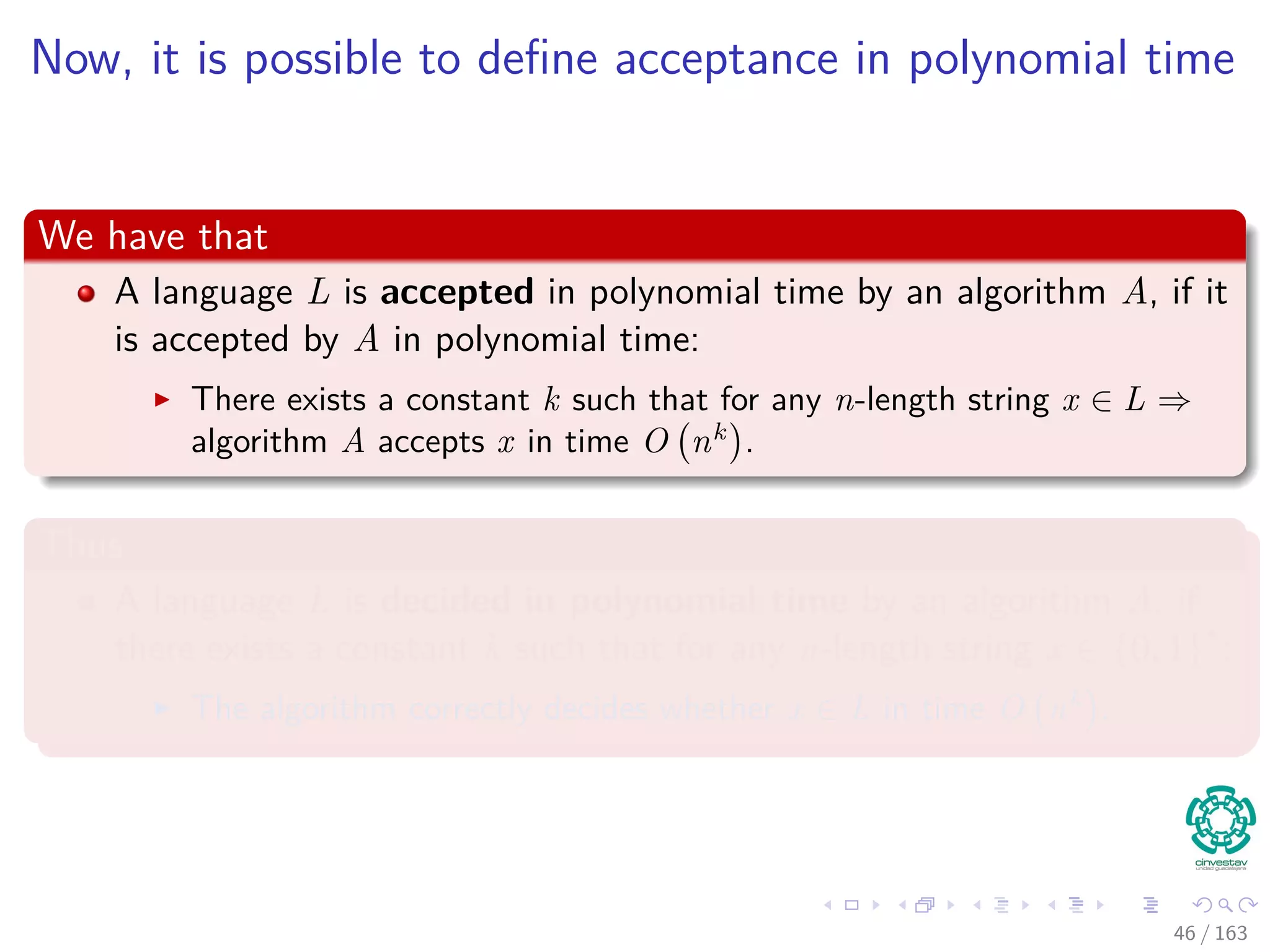
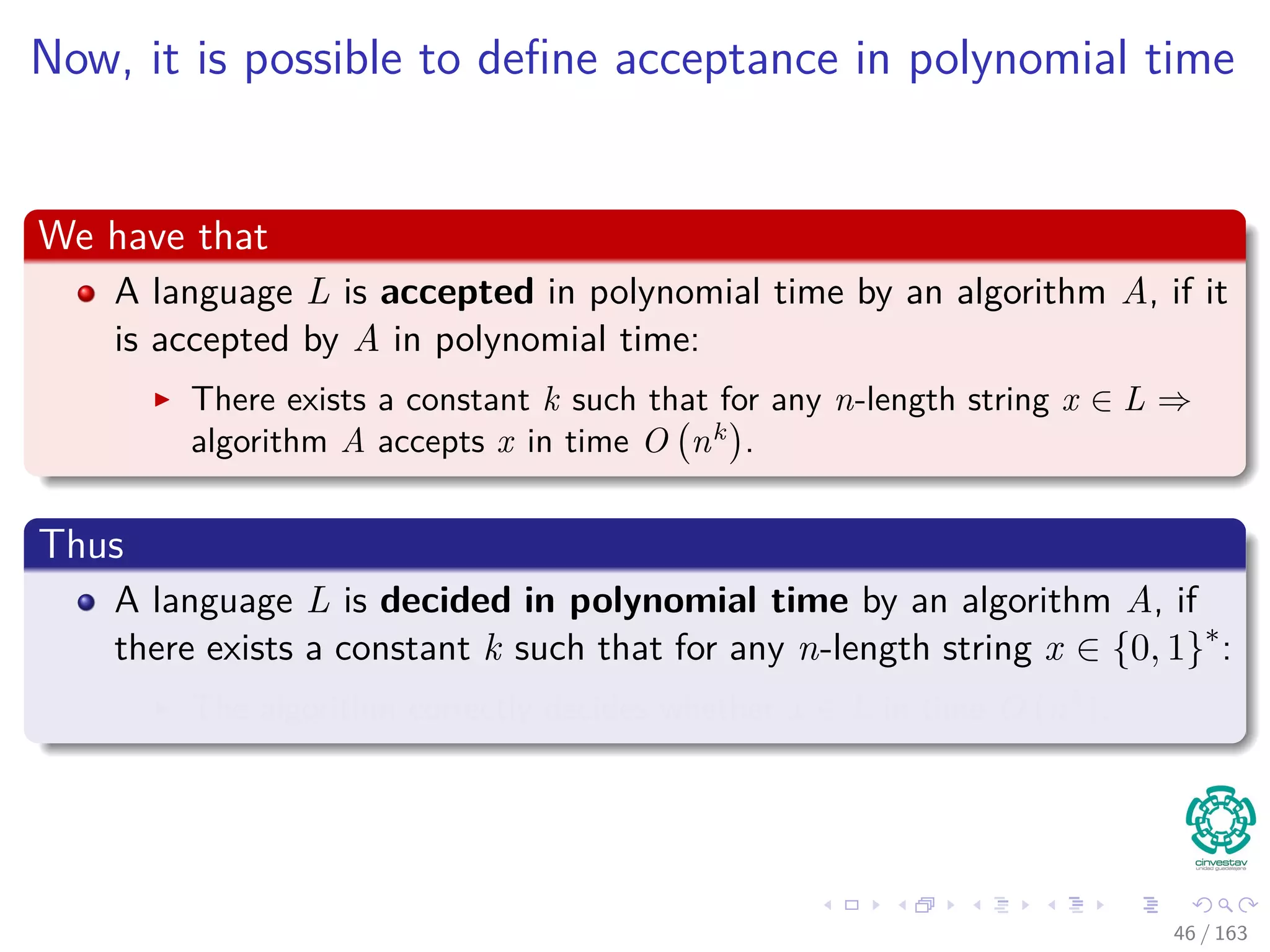
We have the following optimization problem
min
t
d [t]
s.t.d[v] ≤ d[u] + w(u, v) for each edge (u, v) ∈ E
d [s] = 0
Then, we have the following decision problem
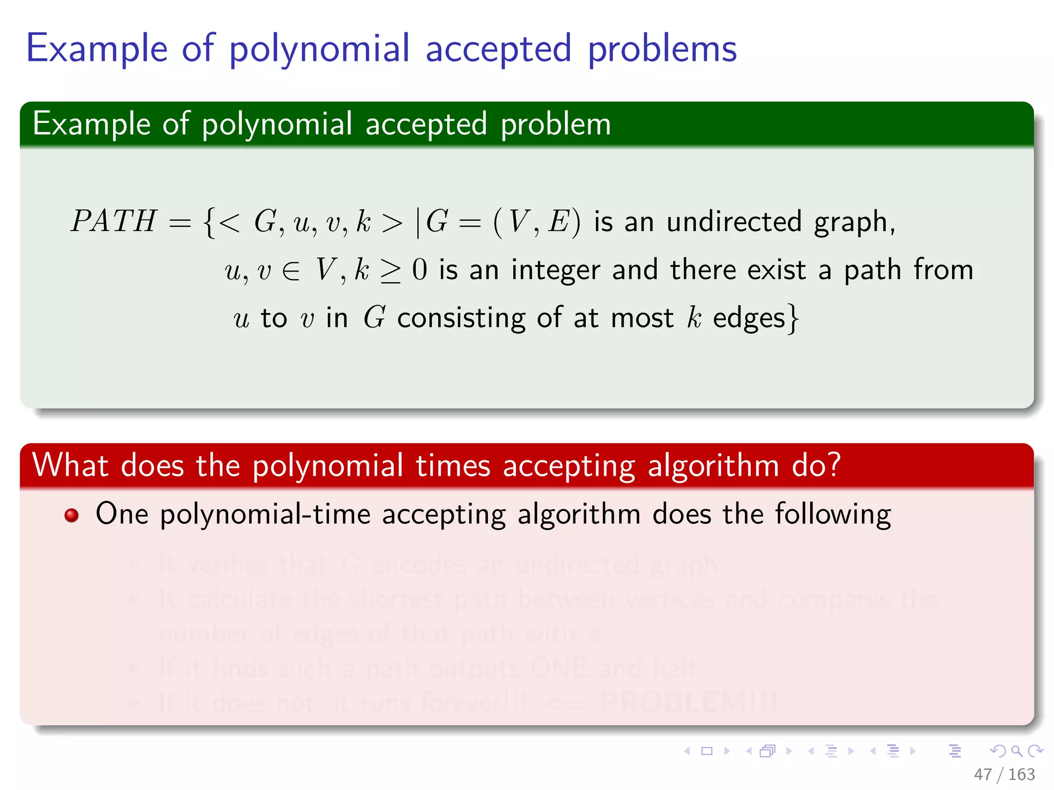
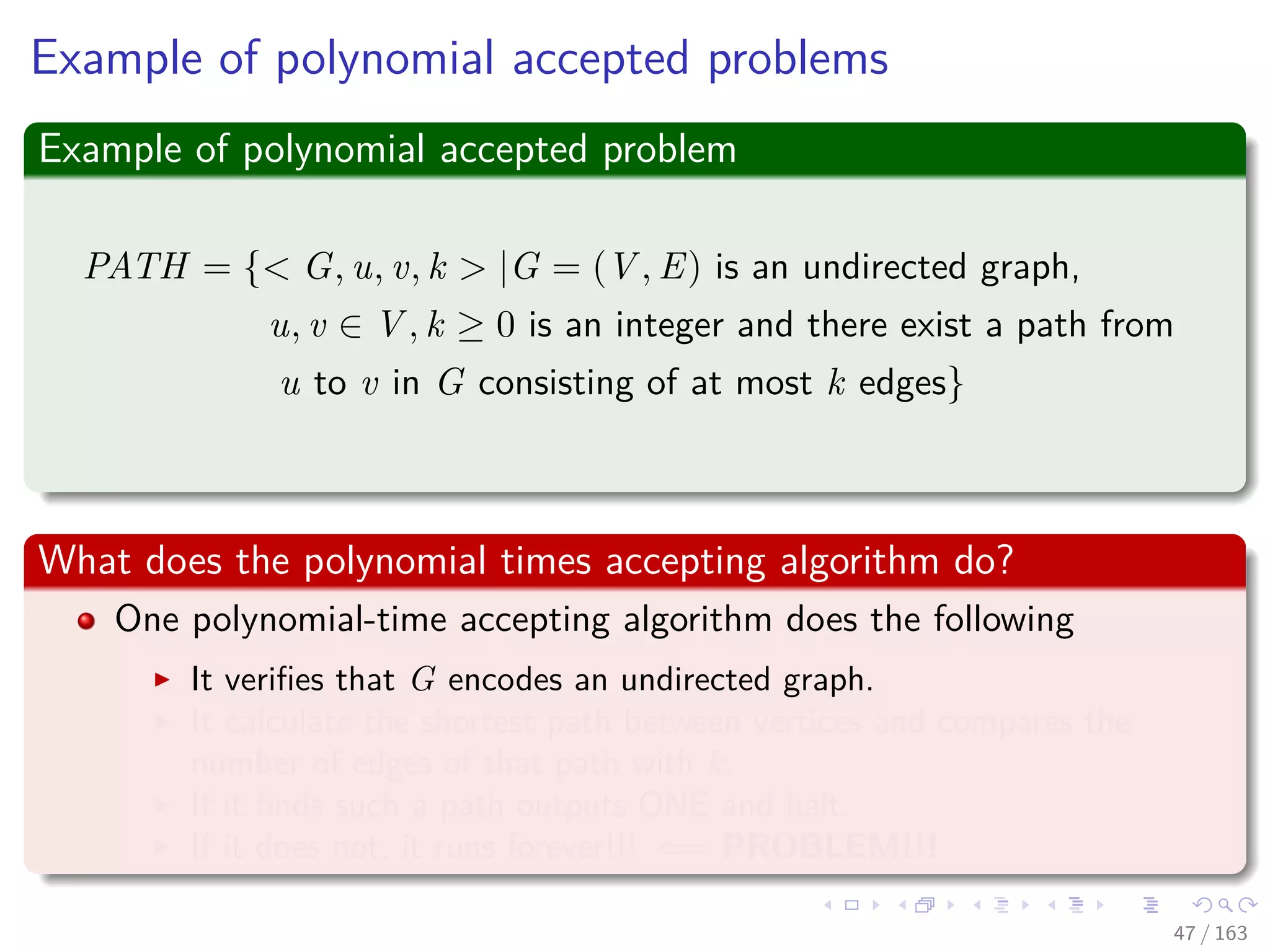
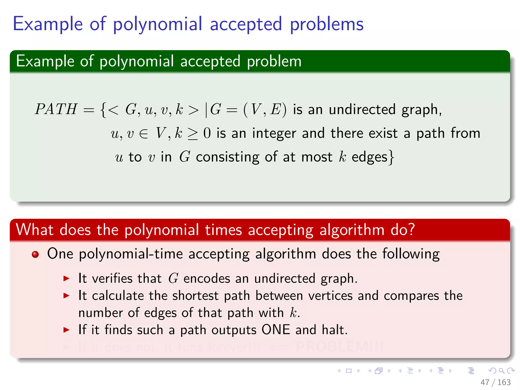
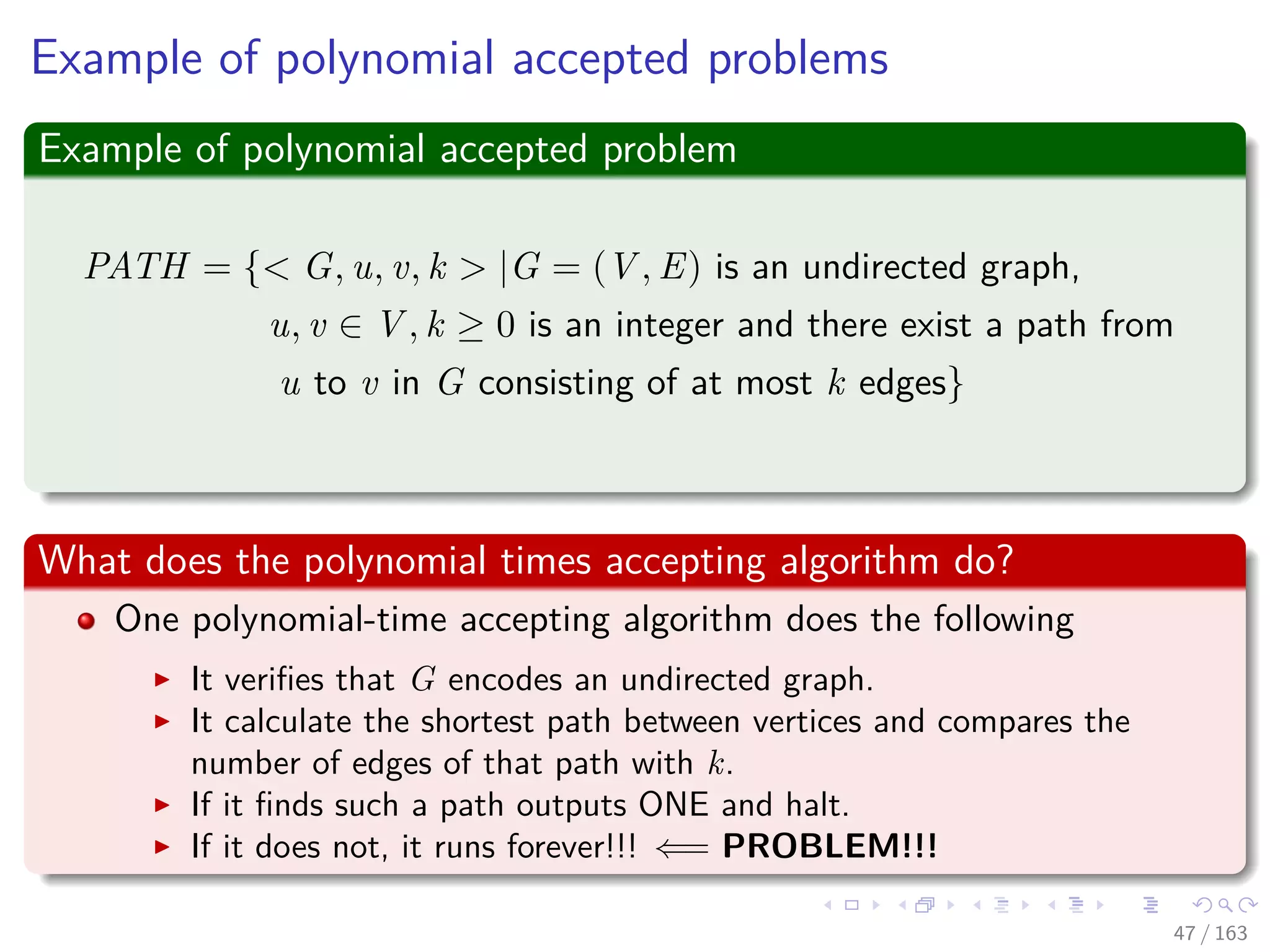
PATH = { G, u, v, k |G = (V , E) is an undirected graph,
u, v ∈ V , k ≥ 0 is an integer and there exist a path from
u to v in G consisting of at most k edges}
22 / 163](https://image.slidesharecdn.com/27npcompletness-151117121725-lva1-app6891/75/27-NP-Completness-40-2048.jpg)
![In a more formal way
We have the following optimization problem
min
t
d [t]
s.t.d[v] ≤ d[u] + w(u, v) for each edge (u, v) ∈ E
d [s] = 0
Then, we have the following decision problem
PATH = { G, u, v, k |G = (V , E) is an undirected graph,
u, v ∈ V , k ≥ 0 is an integer and there exist a path from
u to v in G consisting of at most k edges}
22 / 163](https://image.slidesharecdn.com/27npcompletness-151117121725-lva1-app6891/75/27-NP-Completness-41-2048.jpg)


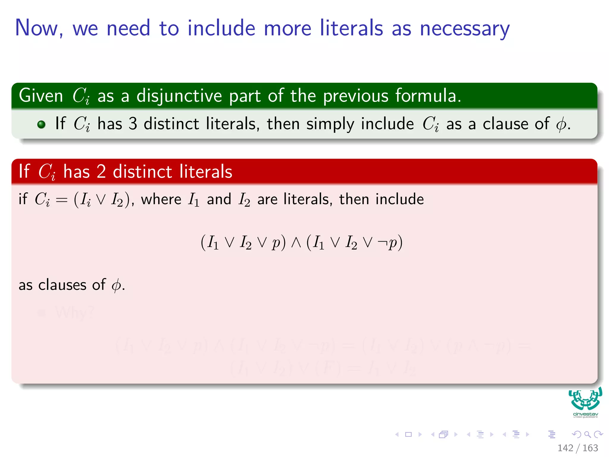
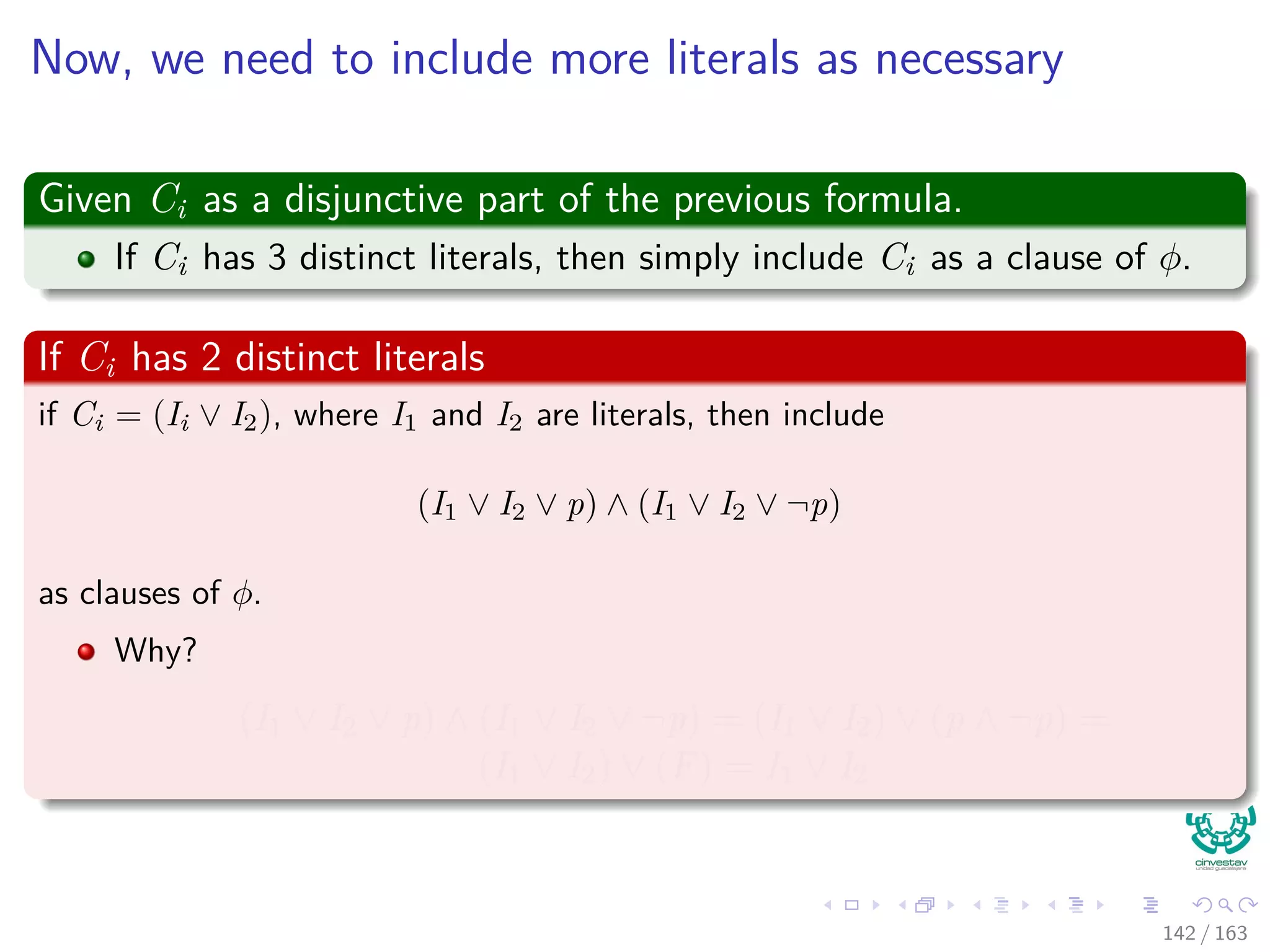
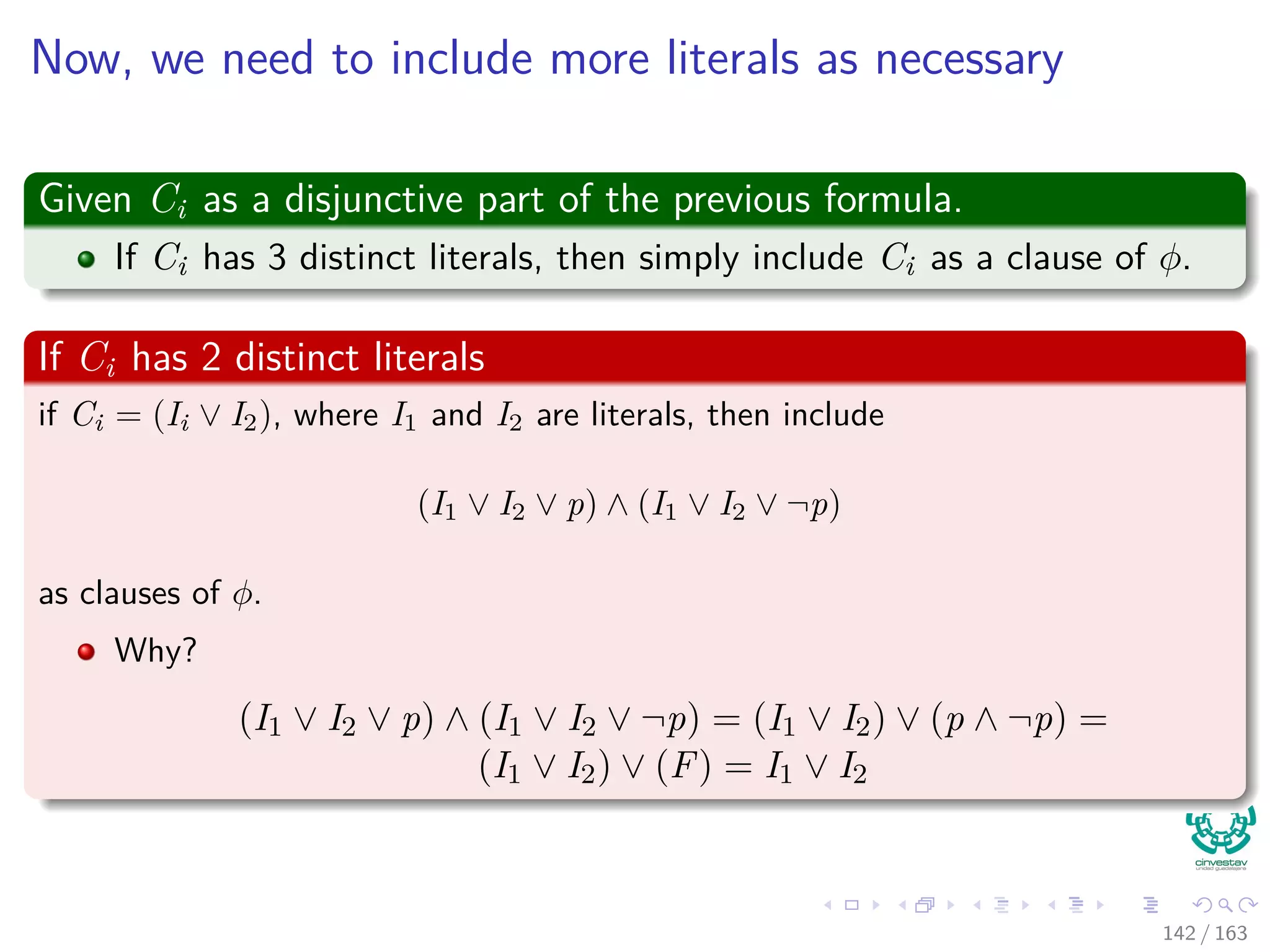
![Now, we need to include more literals as necessary
If Ci has just 1 distinct literal I
Then include (I ∨ p ∨ q) ∧ (I ∨ p ∨ ¬q) ∧ (I ∨ ¬p ∨ q) ∧ (I ∨ ¬p ∨ ¬q)
as clauses of φ.
Why?
(I ∨ p ∨ q) ∧ (I ∨ p ∨ ¬q)∧...
(I ∨ ¬p ∨ q) ∧ (I ∨ ¬p ∨ ¬q) = I ∨ [(p ∨ q) ∧ (p ∨ ¬q) ∧ . . .
(¬p ∨ q) ∧ (¬p ∨ ¬q)]
= I ∨ [p ∨ (q ∧ ¬q) ∧ . . .
(¬p ∨ (q ∧ ¬q))]
= I ∨ [(p ∨ F) ∧ (¬p ∨ F)]
= I ∨ [p ∧ ¬p]
= I ∨ F = I
143 / 163](https://image.slidesharecdn.com/27npcompletness-151117121725-lva1-app6891/75/27-NP-Completness-353-2048.jpg)
![Now, we need to include more literals as necessary
If Ci has just 1 distinct literal I
Then include (I ∨ p ∨ q) ∧ (I ∨ p ∨ ¬q) ∧ (I ∨ ¬p ∨ q) ∧ (I ∨ ¬p ∨ ¬q)
as clauses of φ.
Why?
(I ∨ p ∨ q) ∧ (I ∨ p ∨ ¬q)∧...
(I ∨ ¬p ∨ q) ∧ (I ∨ ¬p ∨ ¬q) = I ∨ [(p ∨ q) ∧ (p ∨ ¬q) ∧ . . .
(¬p ∨ q) ∧ (¬p ∨ ¬q)]
= I ∨ [p ∨ (q ∧ ¬q) ∧ . . .
(¬p ∨ (q ∧ ¬q))]
= I ∨ [(p ∨ F) ∧ (¬p ∨ F)]
= I ∨ [p ∧ ¬p]
= I ∨ F = I
143 / 163](https://image.slidesharecdn.com/27npcompletness-151117121725-lva1-app6891/75/27-NP-Completness-354-2048.jpg)
![Now, we need to include more literals as necessary
If Ci has just 1 distinct literal I
Then include (I ∨ p ∨ q) ∧ (I ∨ p ∨ ¬q) ∧ (I ∨ ¬p ∨ q) ∧ (I ∨ ¬p ∨ ¬q)
as clauses of φ.
Why?
(I ∨ p ∨ q) ∧ (I ∨ p ∨ ¬q)∧...
(I ∨ ¬p ∨ q) ∧ (I ∨ ¬p ∨ ¬q) = I ∨ [(p ∨ q) ∧ (p ∨ ¬q) ∧ . . .
(¬p ∨ q) ∧ (¬p ∨ ¬q)]
= I ∨ [p ∨ (q ∧ ¬q) ∧ . . .
(¬p ∨ (q ∧ ¬q))]
= I ∨ [(p ∨ F) ∧ (¬p ∨ F)]
= I ∨ [p ∧ ¬p]
= I ∨ F = I
143 / 163](https://image.slidesharecdn.com/27npcompletness-151117121725-lva1-app6891/75/27-NP-Completness-355-2048.jpg)
![Now, we need to include more literals as necessary
If Ci has just 1 distinct literal I
Then include (I ∨ p ∨ q) ∧ (I ∨ p ∨ ¬q) ∧ (I ∨ ¬p ∨ q) ∧ (I ∨ ¬p ∨ ¬q)
as clauses of φ.
Why?
(I ∨ p ∨ q) ∧ (I ∨ p ∨ ¬q)∧...
(I ∨ ¬p ∨ q) ∧ (I ∨ ¬p ∨ ¬q) = I ∨ [(p ∨ q) ∧ (p ∨ ¬q) ∧ . . .
(¬p ∨ q) ∧ (¬p ∨ ¬q)]
= I ∨ [p ∨ (q ∧ ¬q) ∧ . . .
(¬p ∨ (q ∧ ¬q))]
= I ∨ [(p ∨ F) ∧ (¬p ∨ F)]
= I ∨ [p ∧ ¬p]
= I ∨ F = I
143 / 163](https://image.slidesharecdn.com/27npcompletness-151117121725-lva1-app6891/75/27-NP-Completness-356-2048.jpg)
![Now, we need to include more literals as necessary
If Ci has just 1 distinct literal I
Then include (I ∨ p ∨ q) ∧ (I ∨ p ∨ ¬q) ∧ (I ∨ ¬p ∨ q) ∧ (I ∨ ¬p ∨ ¬q)
as clauses of φ.
Why?
(I ∨ p ∨ q) ∧ (I ∨ p ∨ ¬q)∧...
(I ∨ ¬p ∨ q) ∧ (I ∨ ¬p ∨ ¬q) = I ∨ [(p ∨ q) ∧ (p ∨ ¬q) ∧ . . .
(¬p ∨ q) ∧ (¬p ∨ ¬q)]
= I ∨ [p ∨ (q ∧ ¬q) ∧ . . .
(¬p ∨ (q ∧ ¬q))]
= I ∨ [(p ∨ F) ∧ (¬p ∨ F)]
= I ∨ [p ∧ ¬p]
= I ∨ F = I
143 / 163](https://image.slidesharecdn.com/27npcompletness-151117121725-lva1-app6891/75/27-NP-Completness-357-2048.jpg)
![Now, we need to include more literals as necessary
If Ci has just 1 distinct literal I
Then include (I ∨ p ∨ q) ∧ (I ∨ p ∨ ¬q) ∧ (I ∨ ¬p ∨ q) ∧ (I ∨ ¬p ∨ ¬q)
as clauses of φ.
Why?
(I ∨ p ∨ q) ∧ (I ∨ p ∨ ¬q)∧...
(I ∨ ¬p ∨ q) ∧ (I ∨ ¬p ∨ ¬q) = I ∨ [(p ∨ q) ∧ (p ∨ ¬q) ∧ . . .
(¬p ∨ q) ∧ (¬p ∨ ¬q)]
= I ∨ [p ∨ (q ∧ ¬q) ∧ . . .
(¬p ∨ (q ∧ ¬q))]
= I ∨ [(p ∨ F) ∧ (¬p ∨ F)]
= I ∨ [p ∧ ¬p]
= I ∨ F = I
143 / 163](https://image.slidesharecdn.com/27npcompletness-151117121725-lva1-app6891/75/27-NP-Completness-358-2048.jpg)


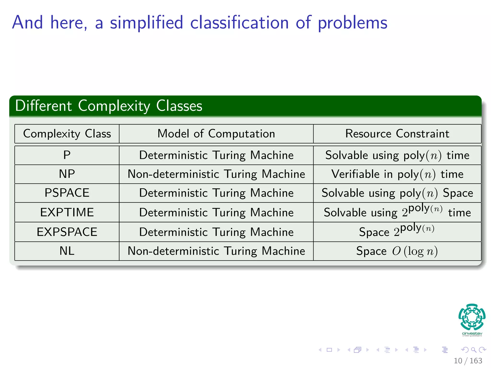
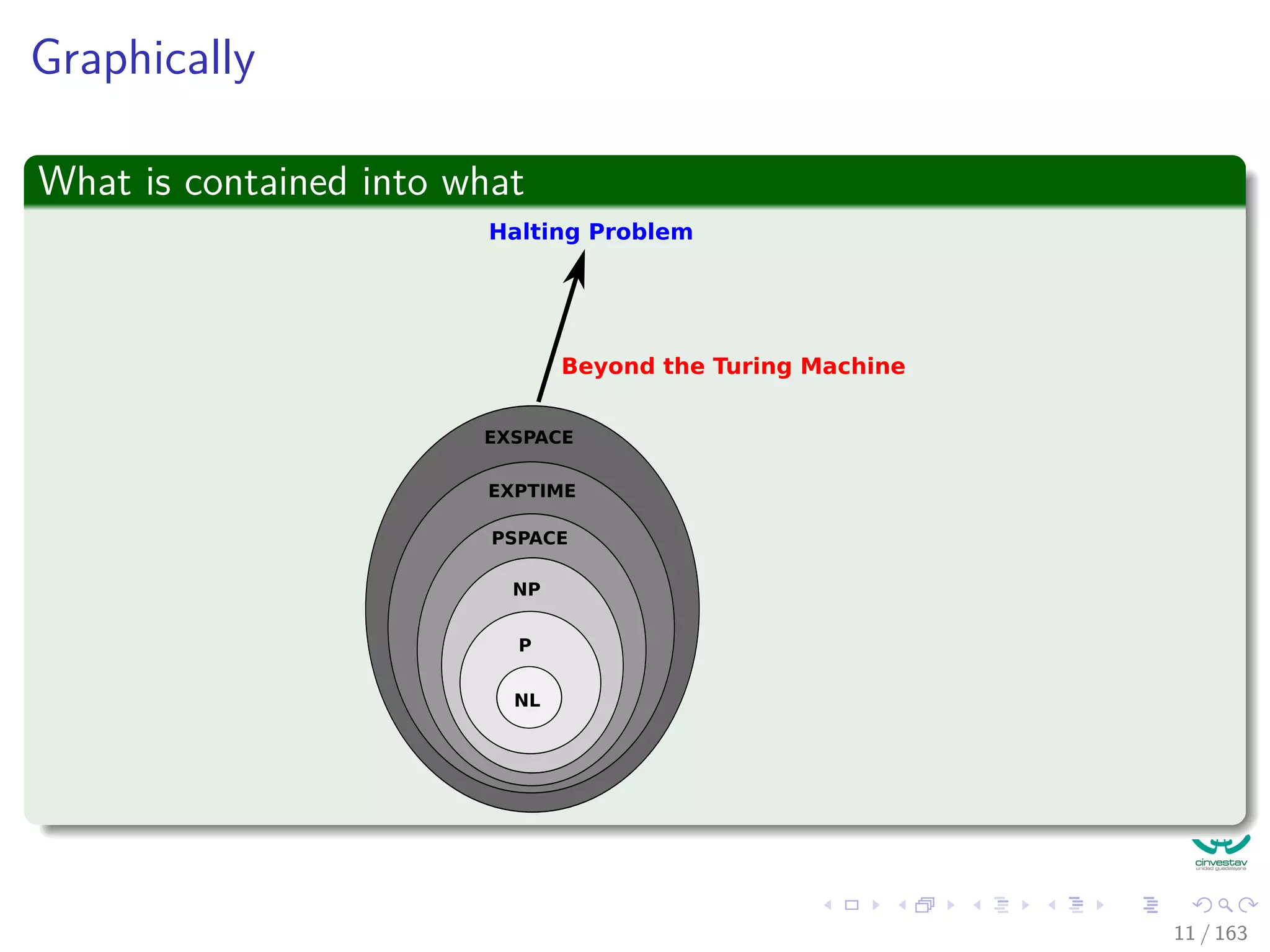
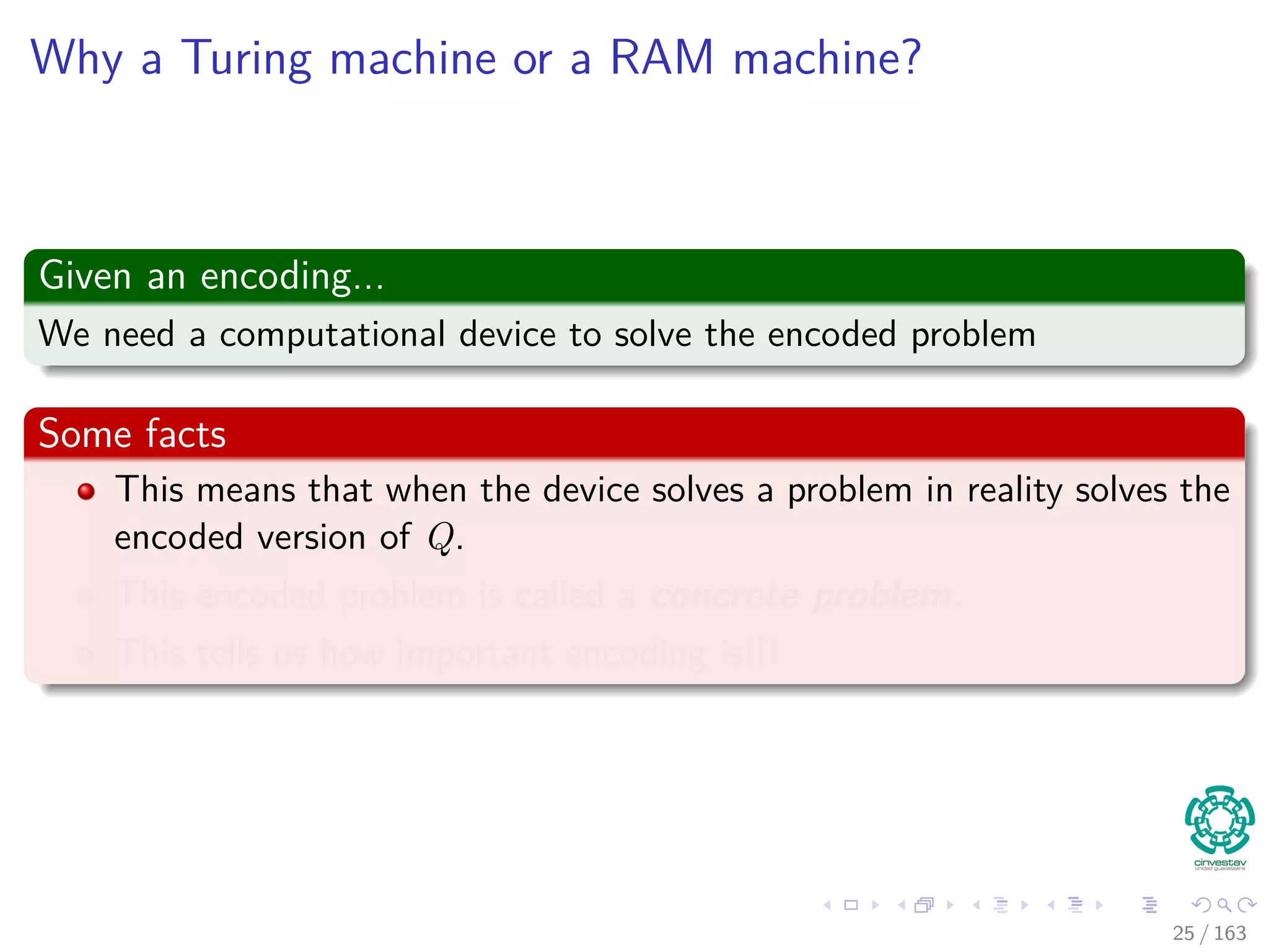
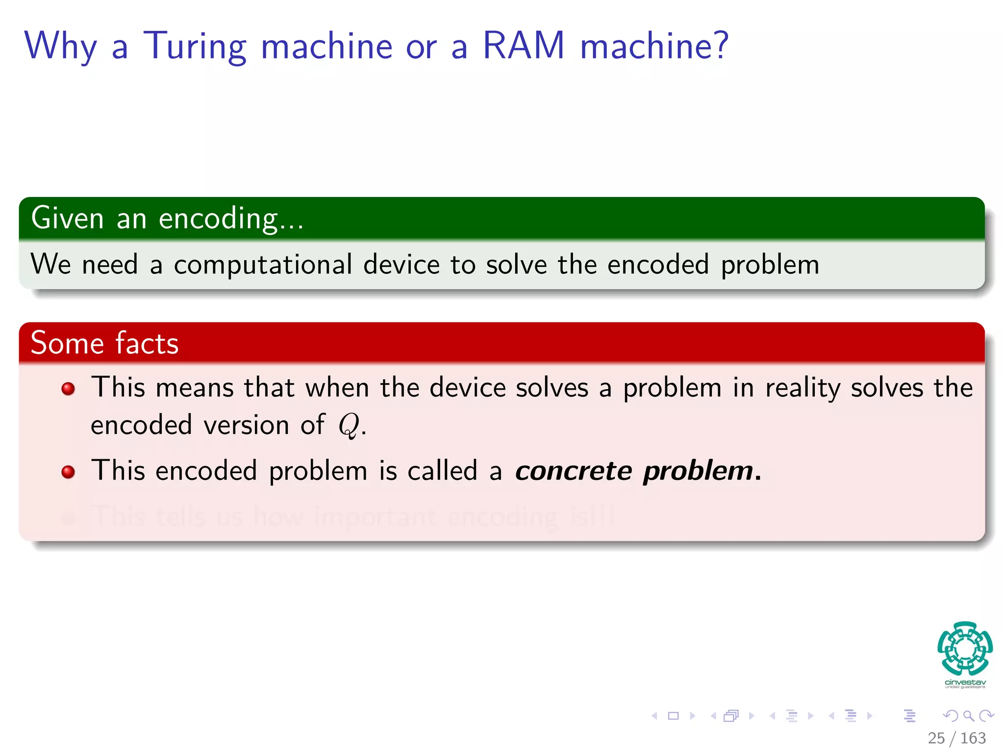
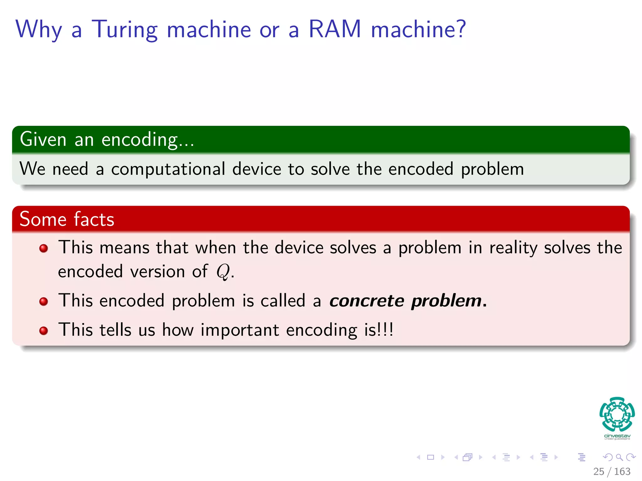
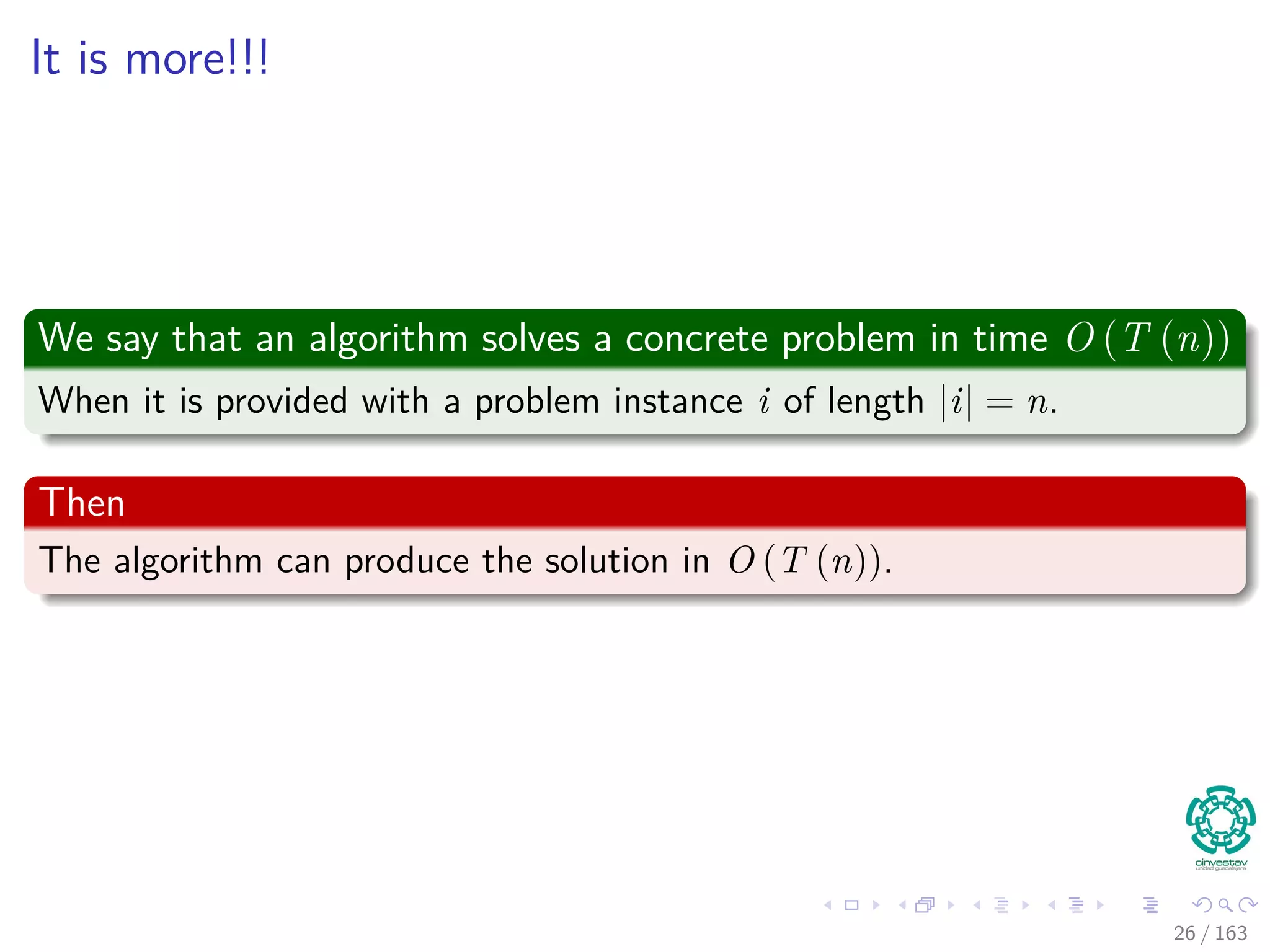
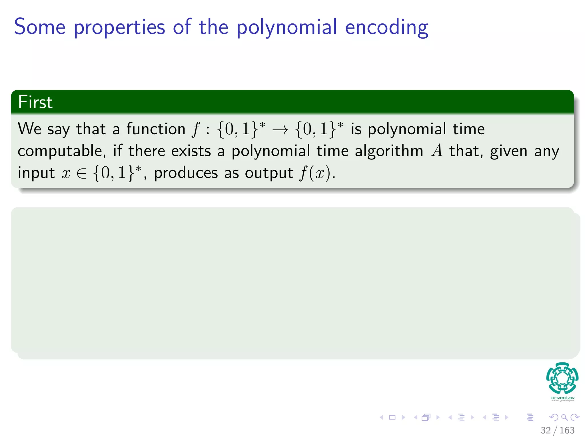
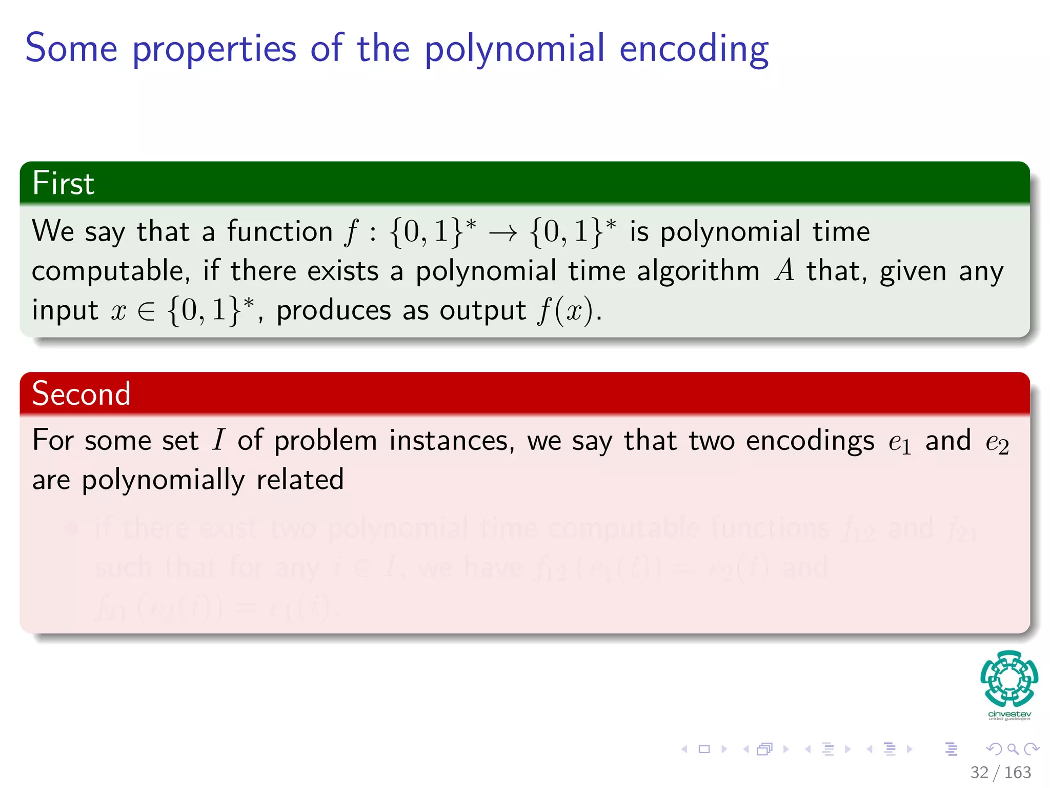
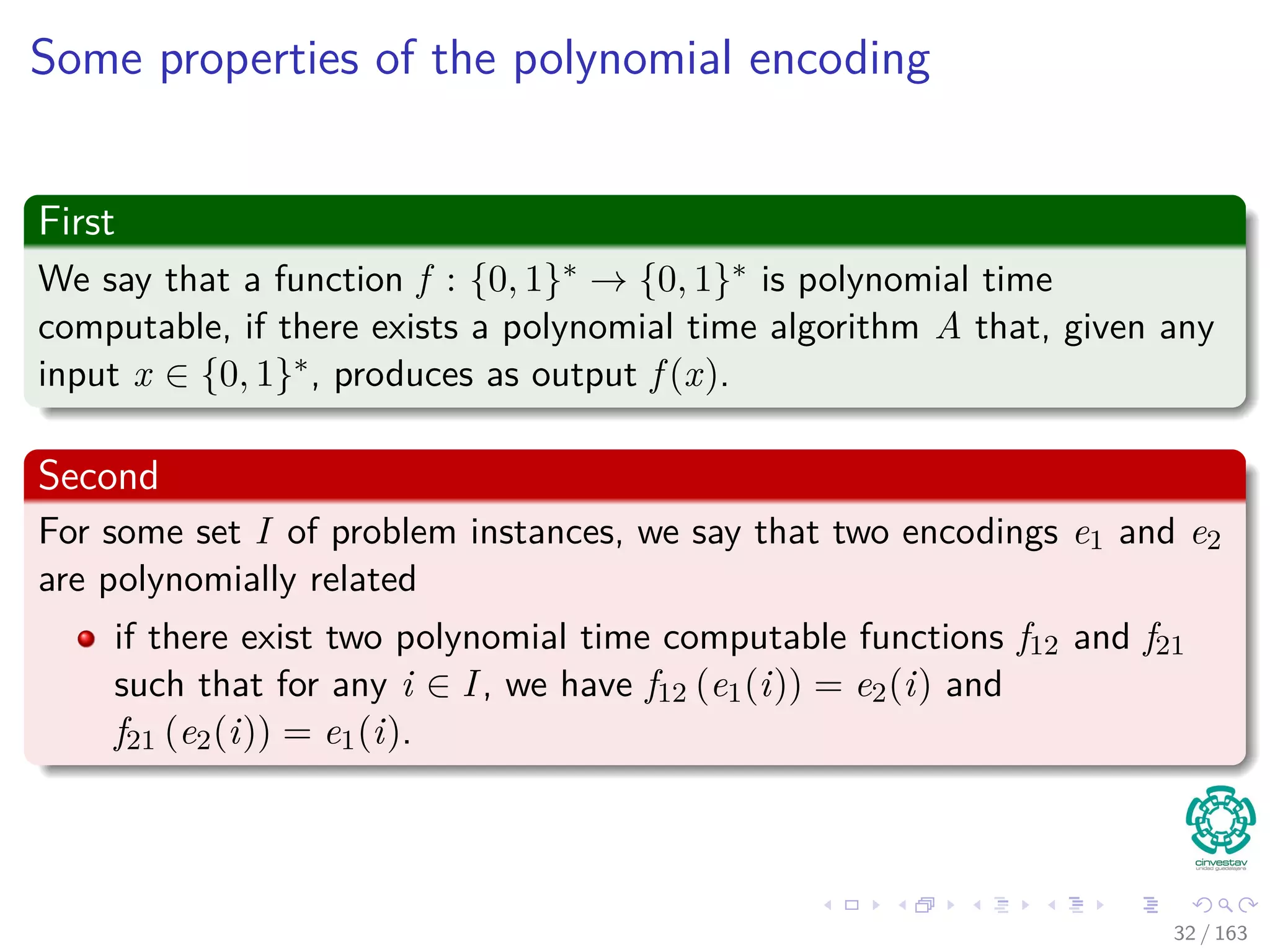
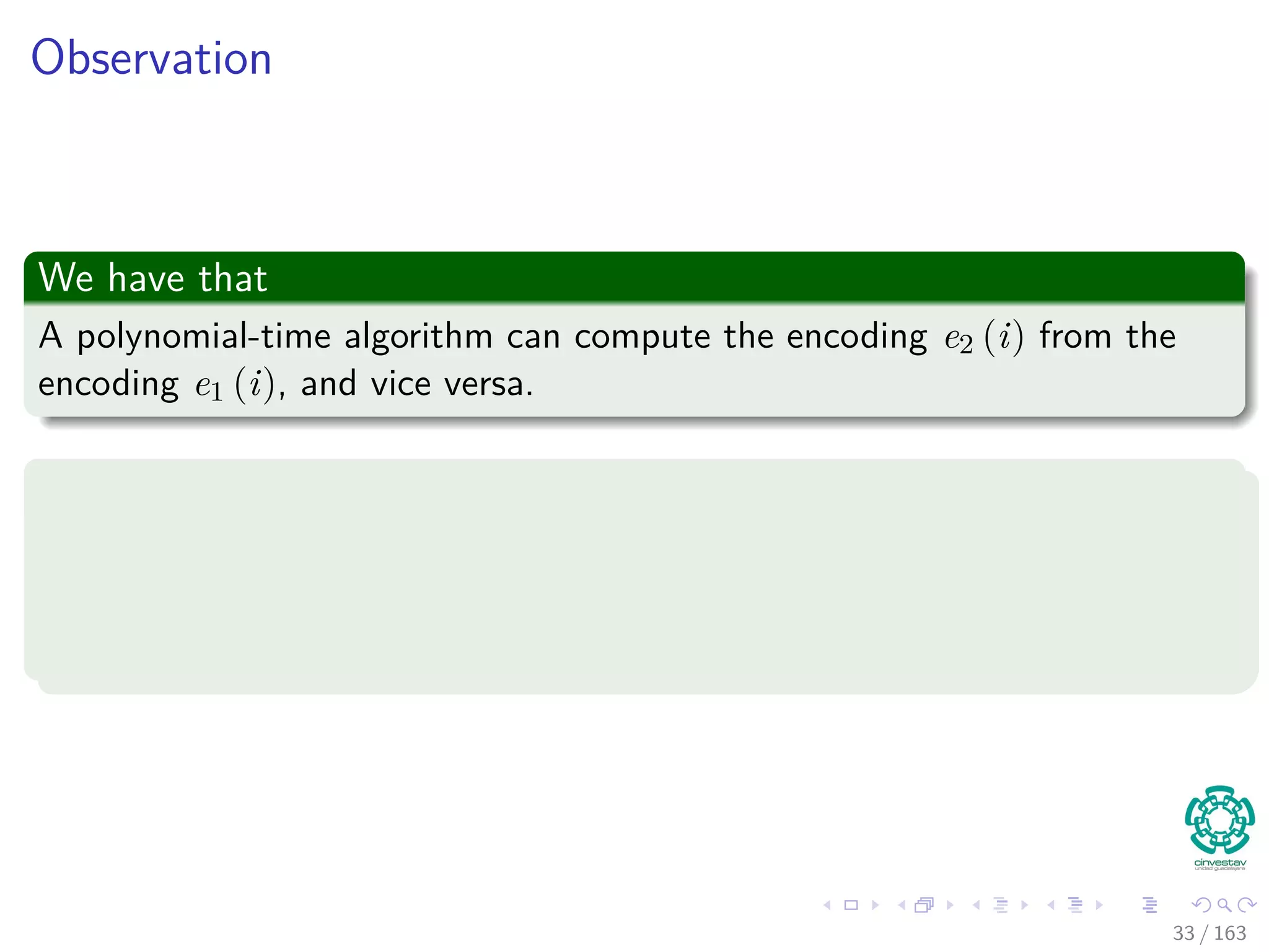
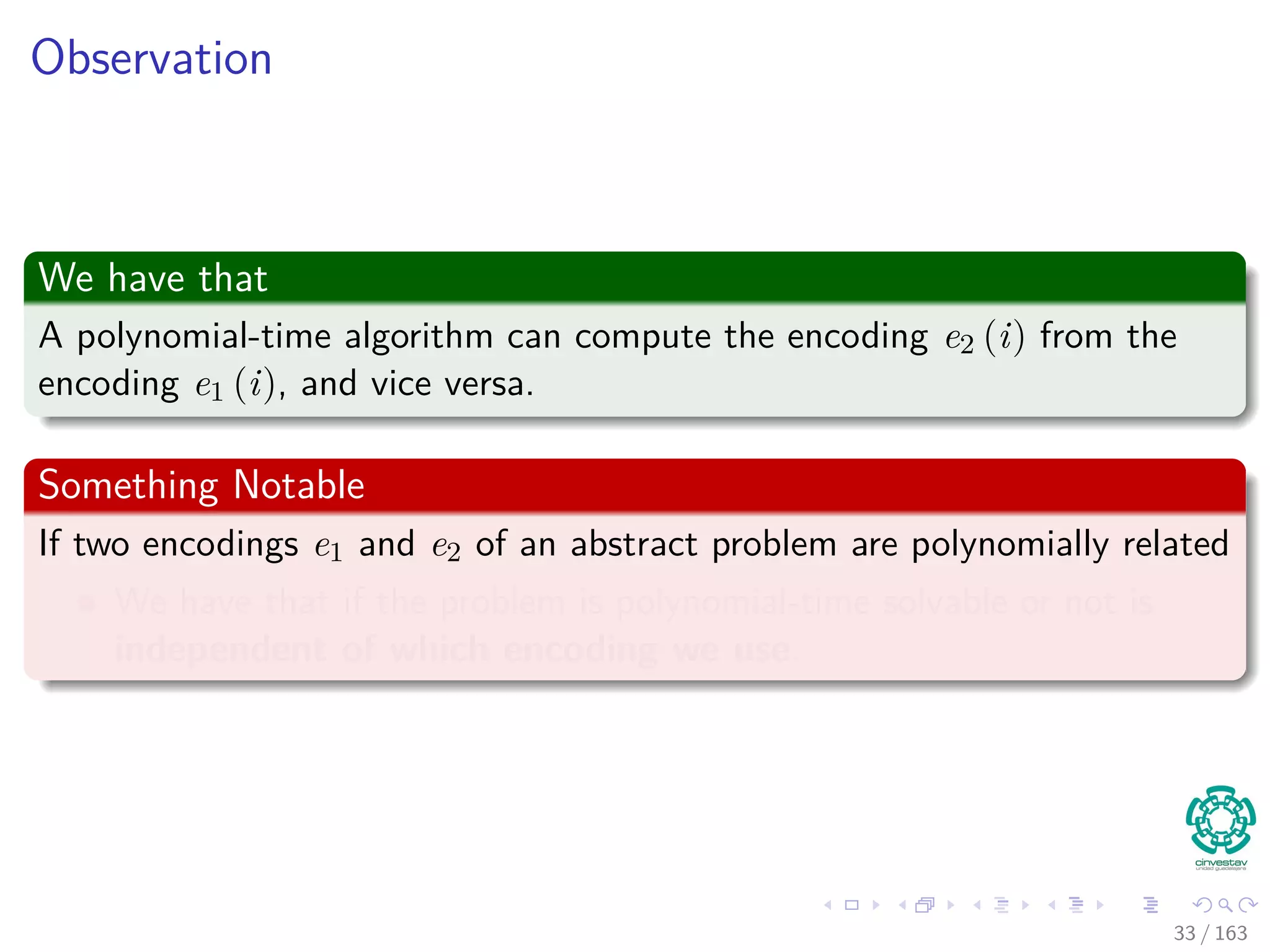
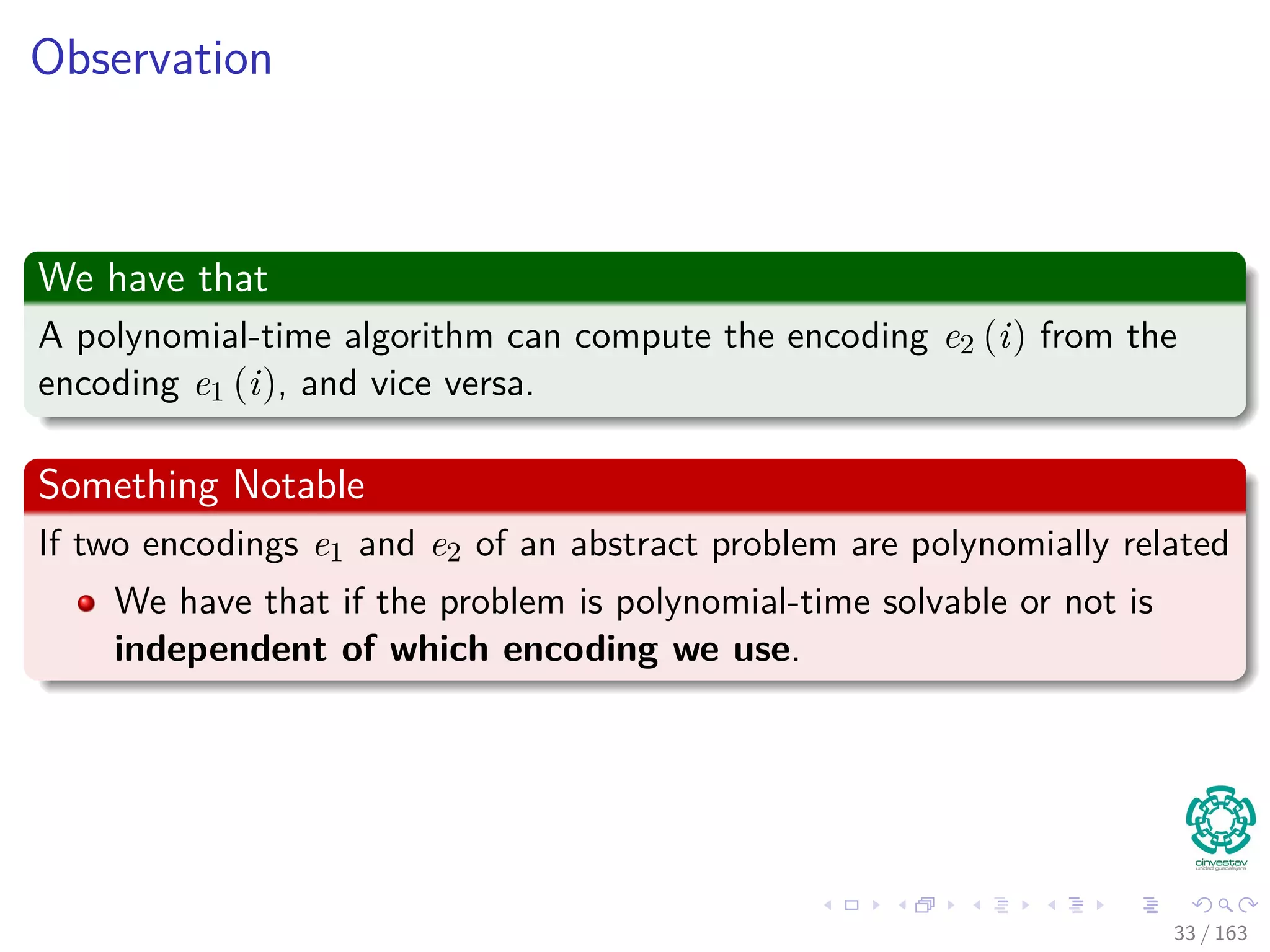
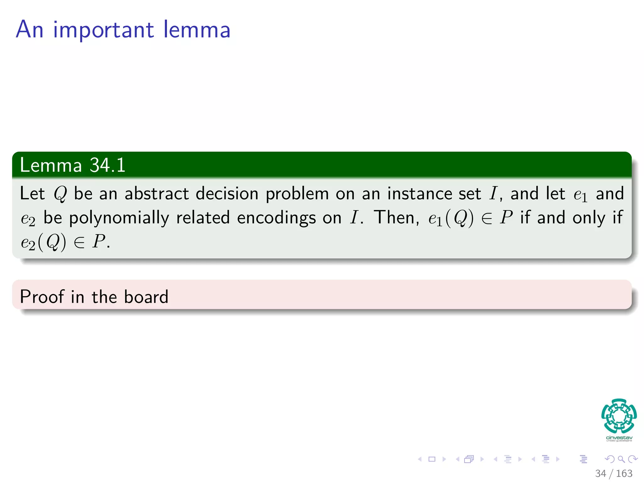
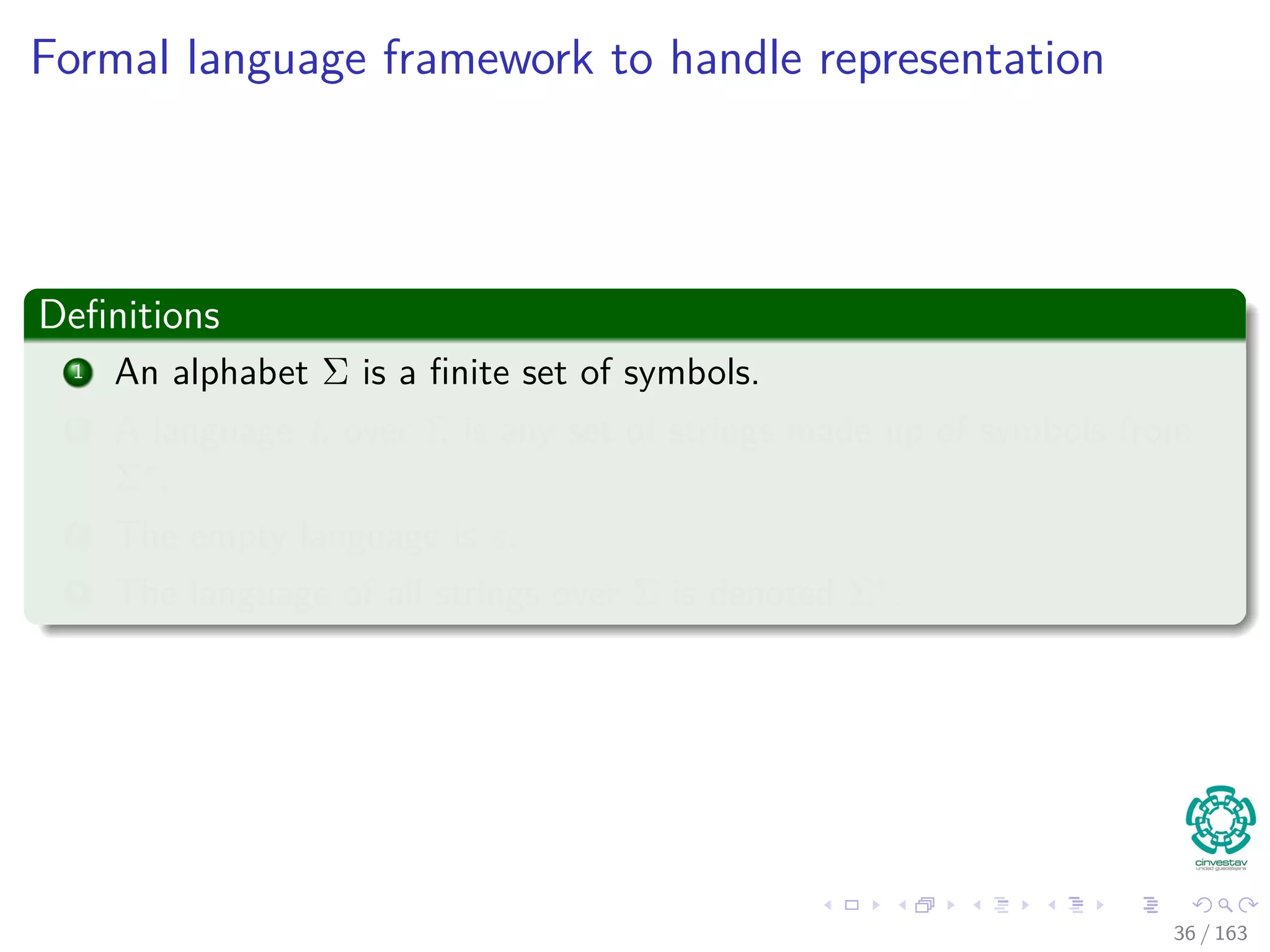
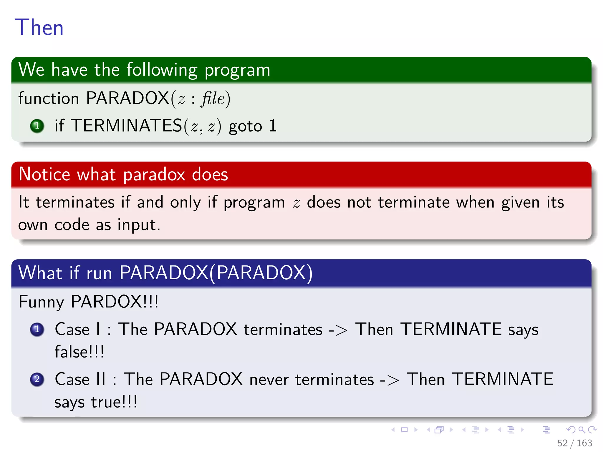
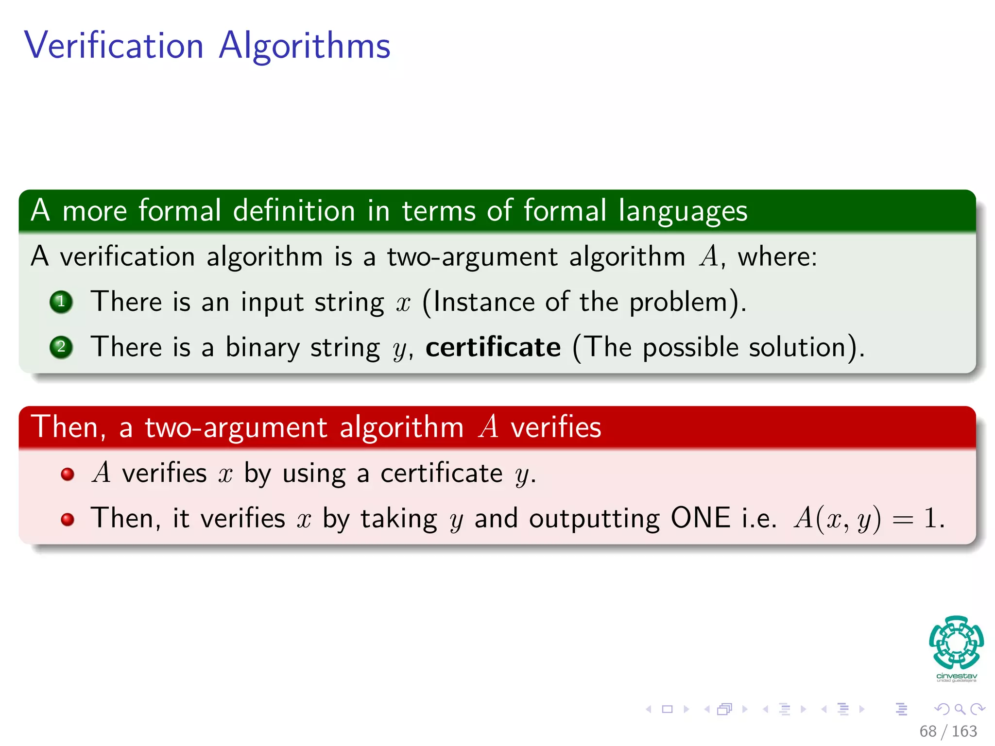
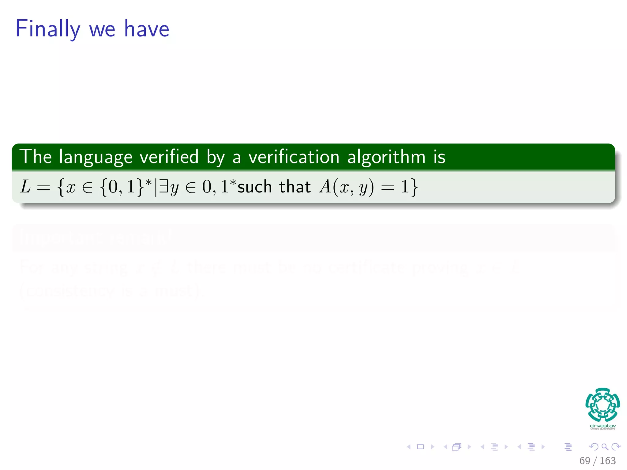
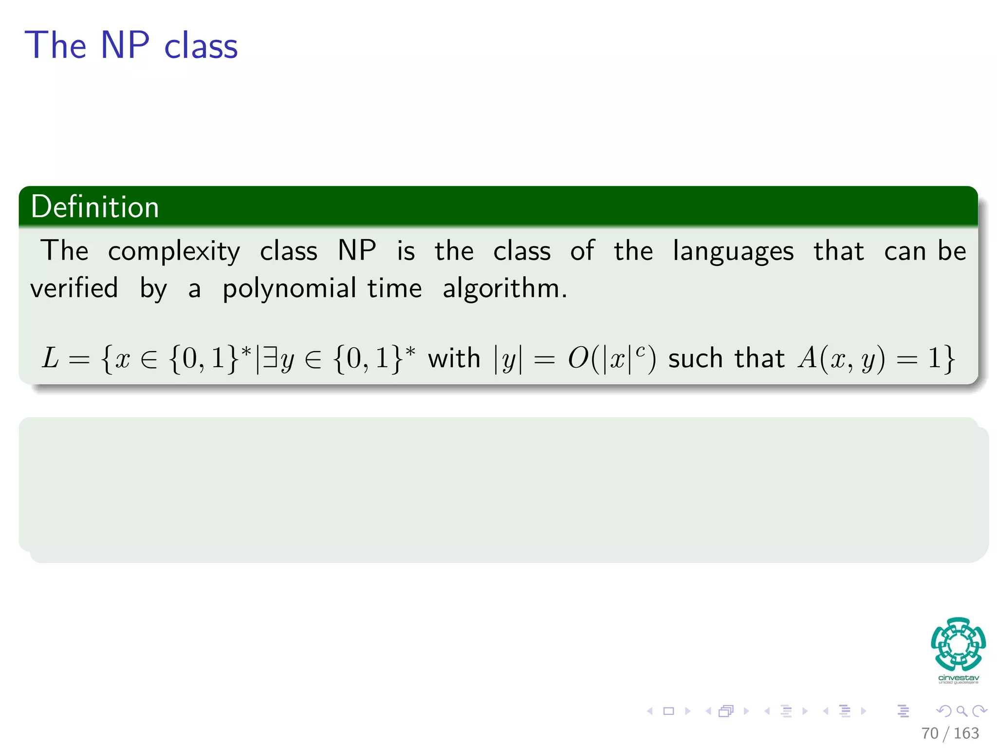
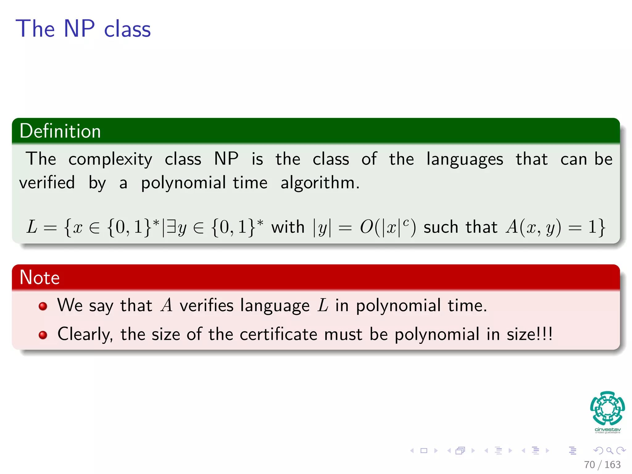
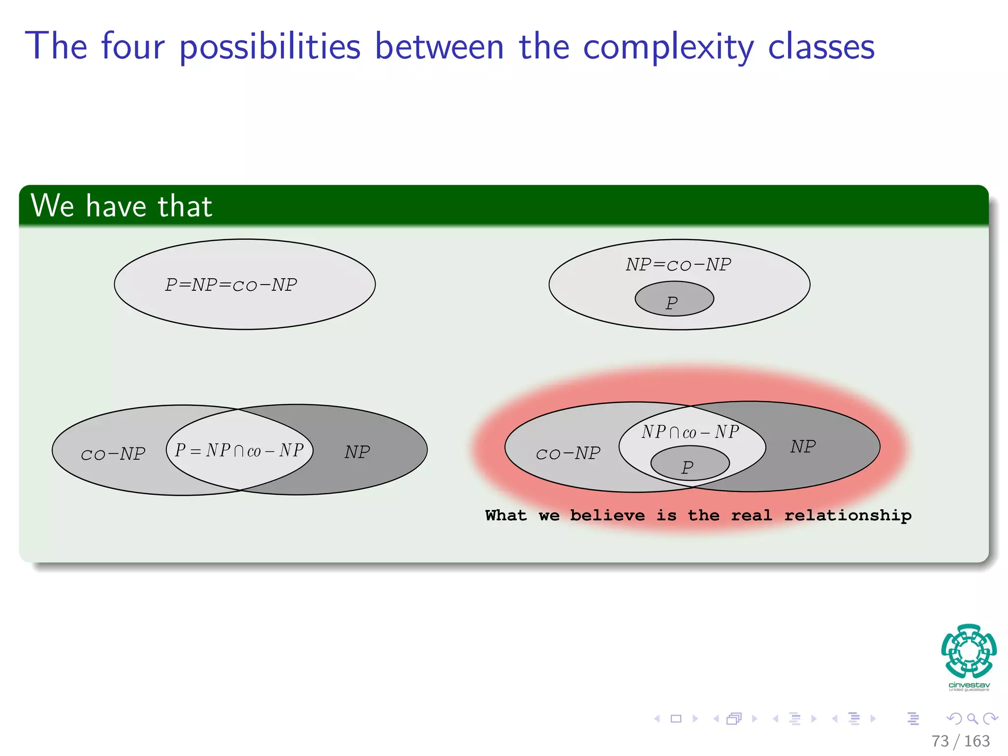
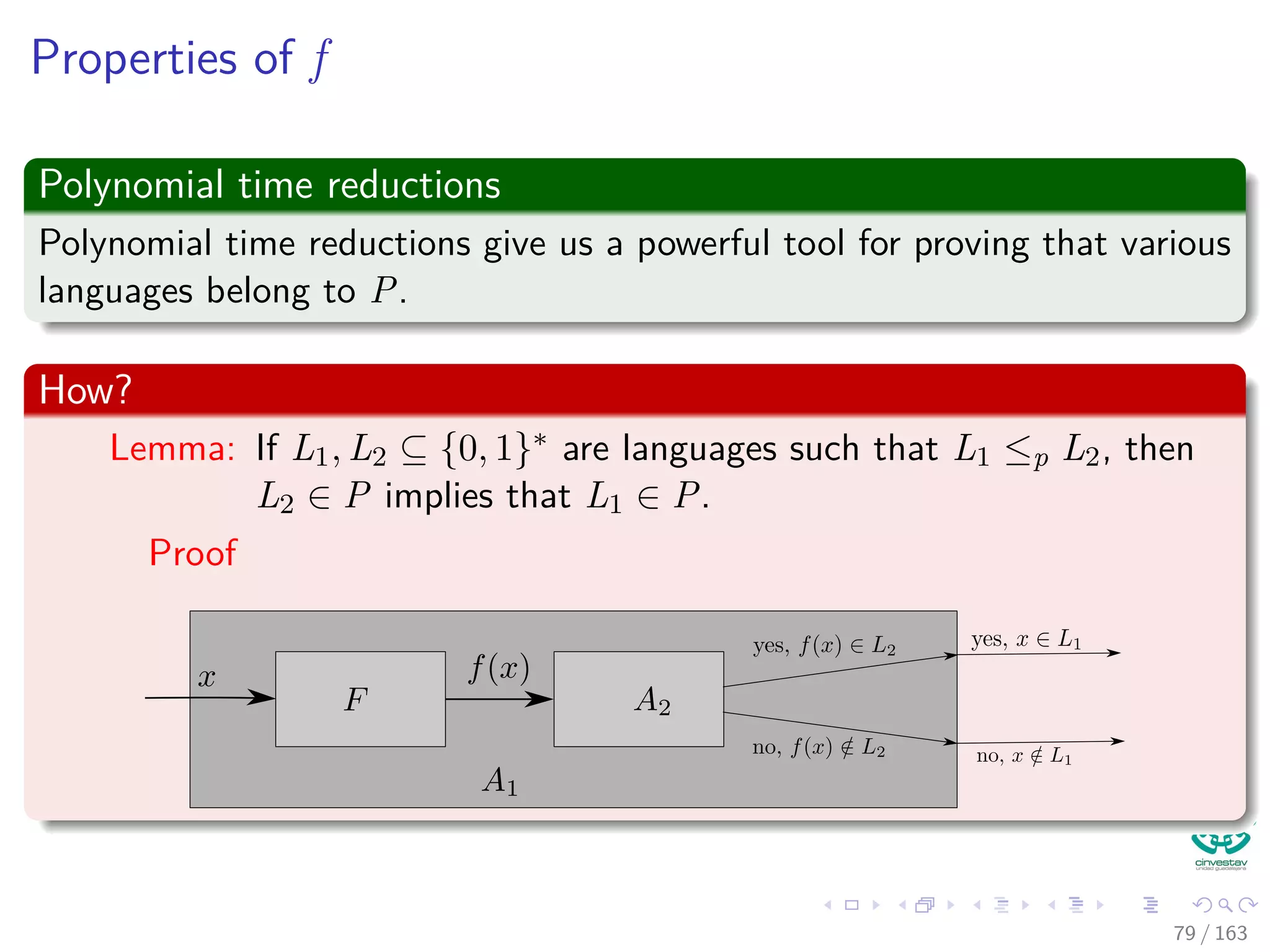
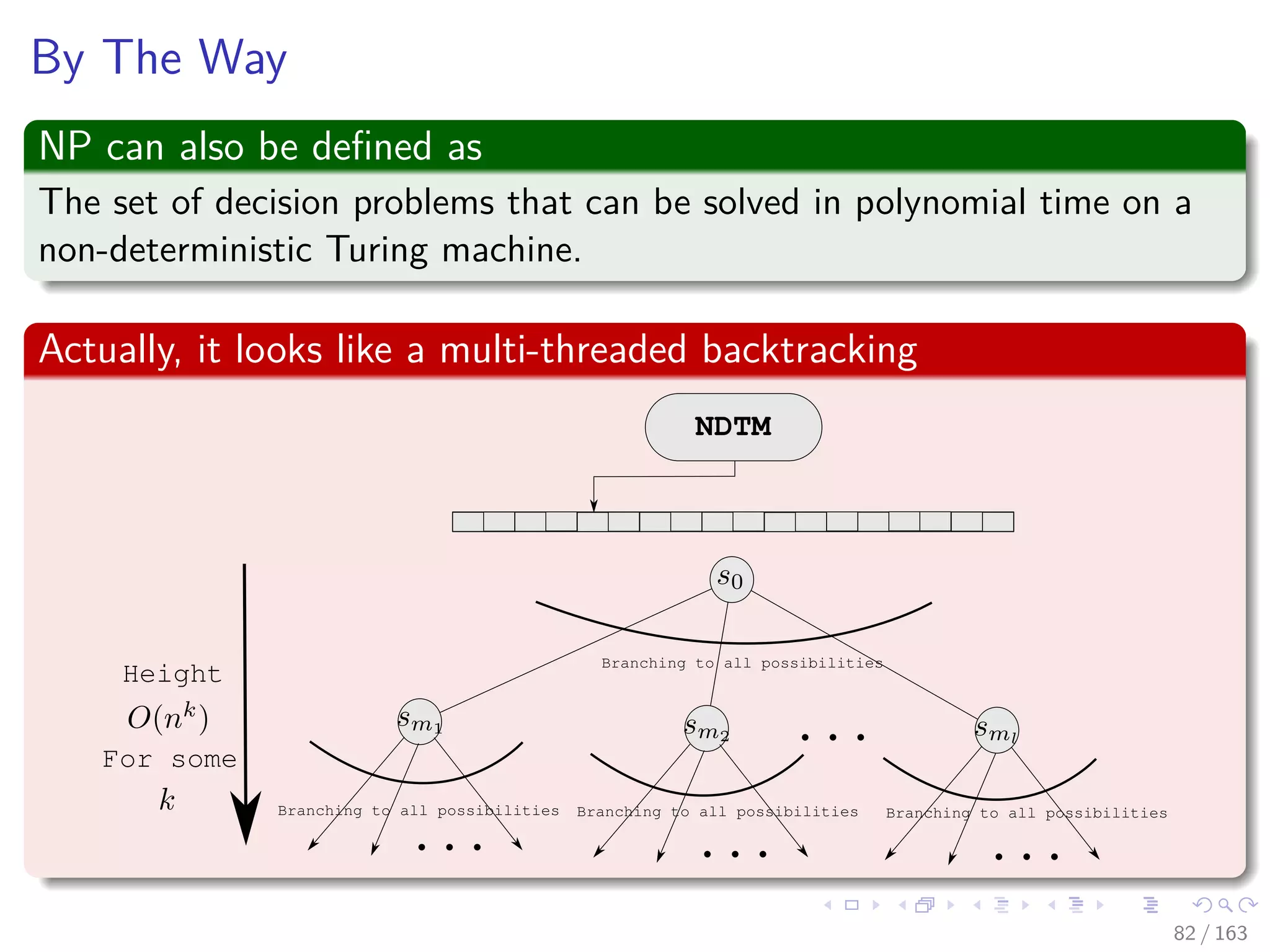
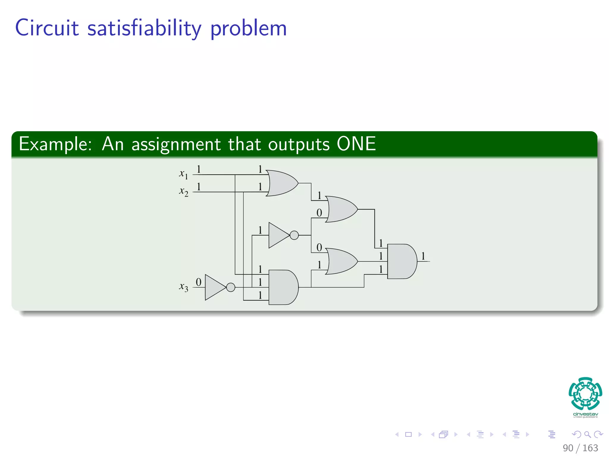
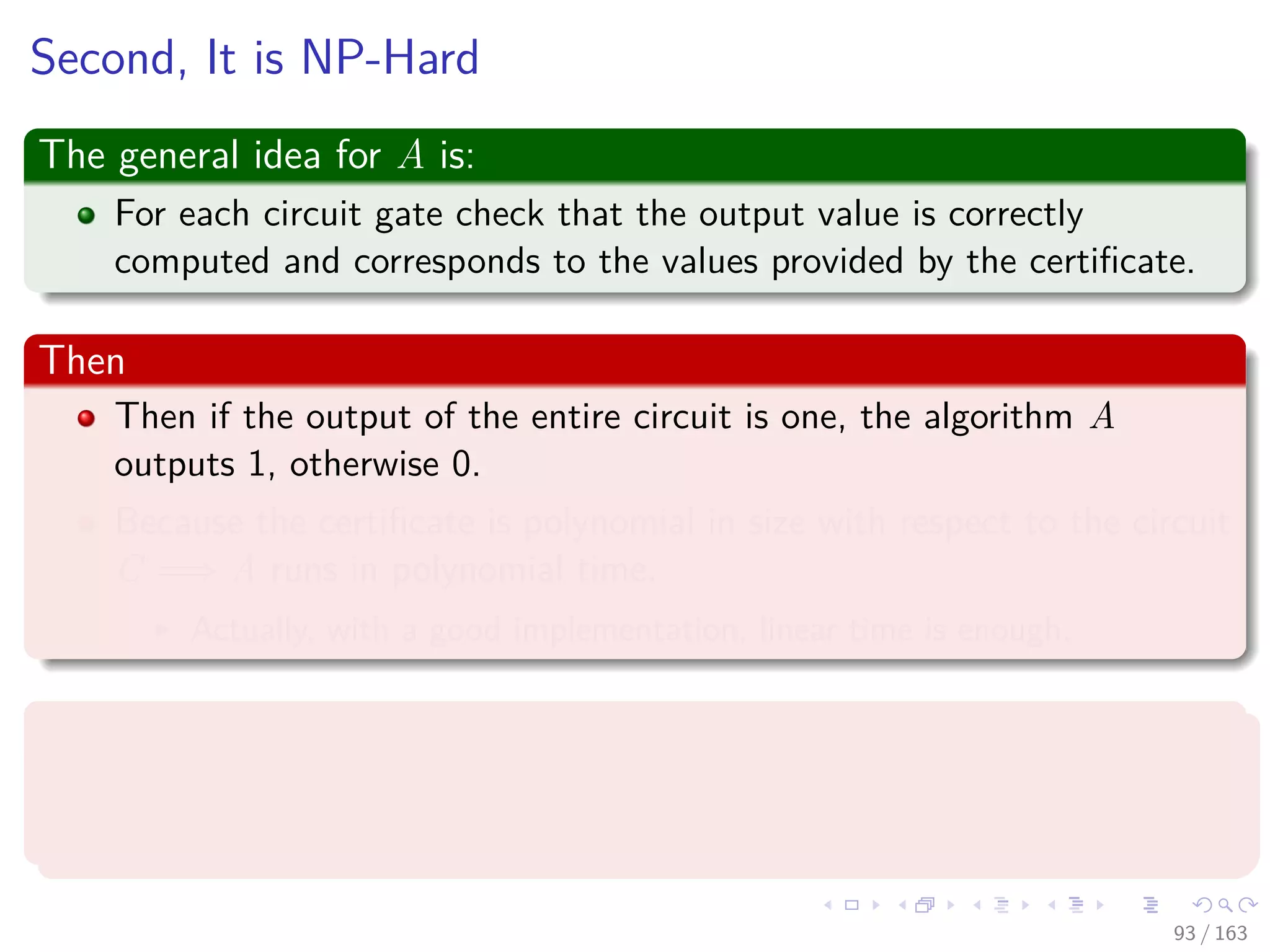
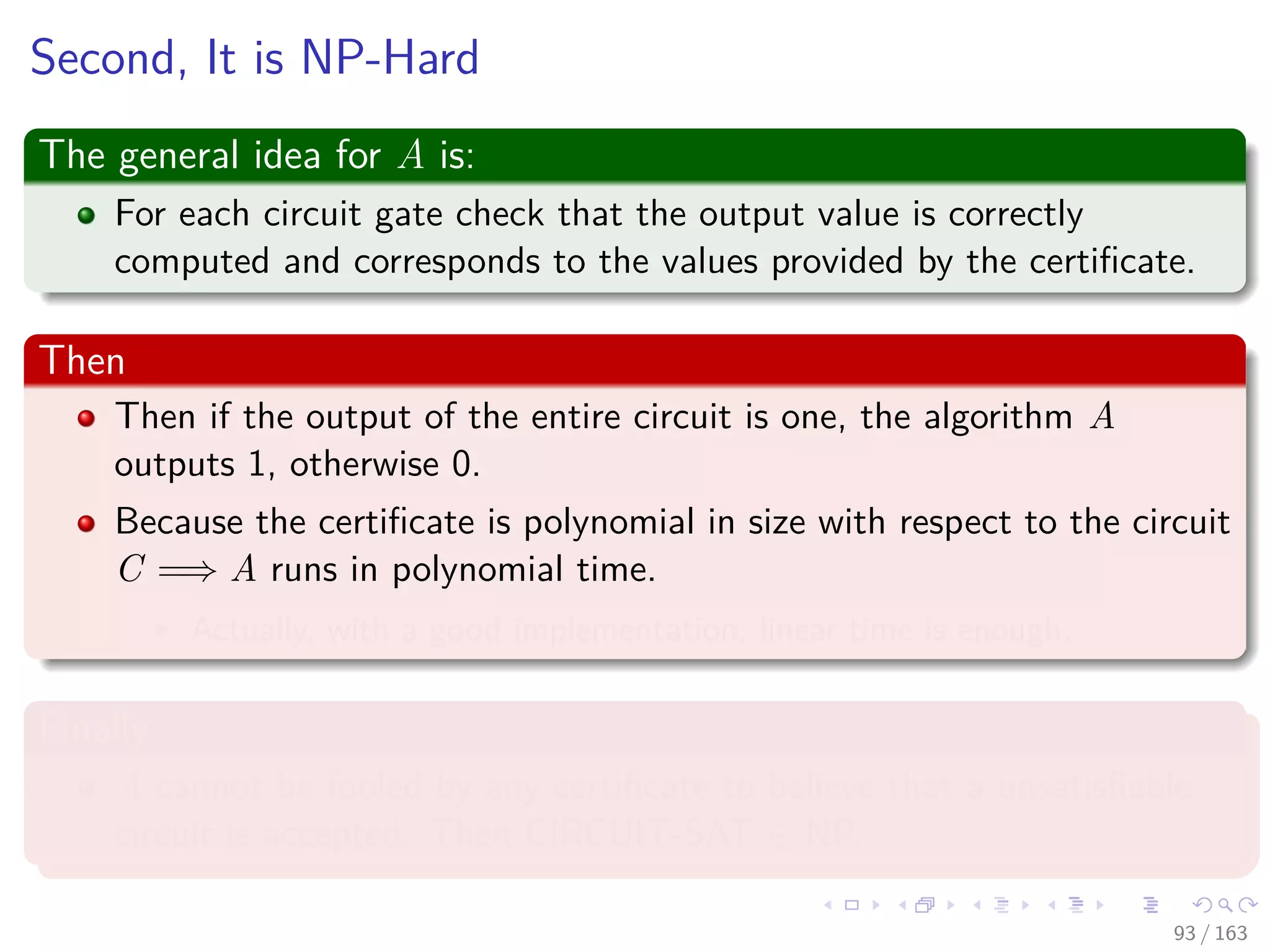
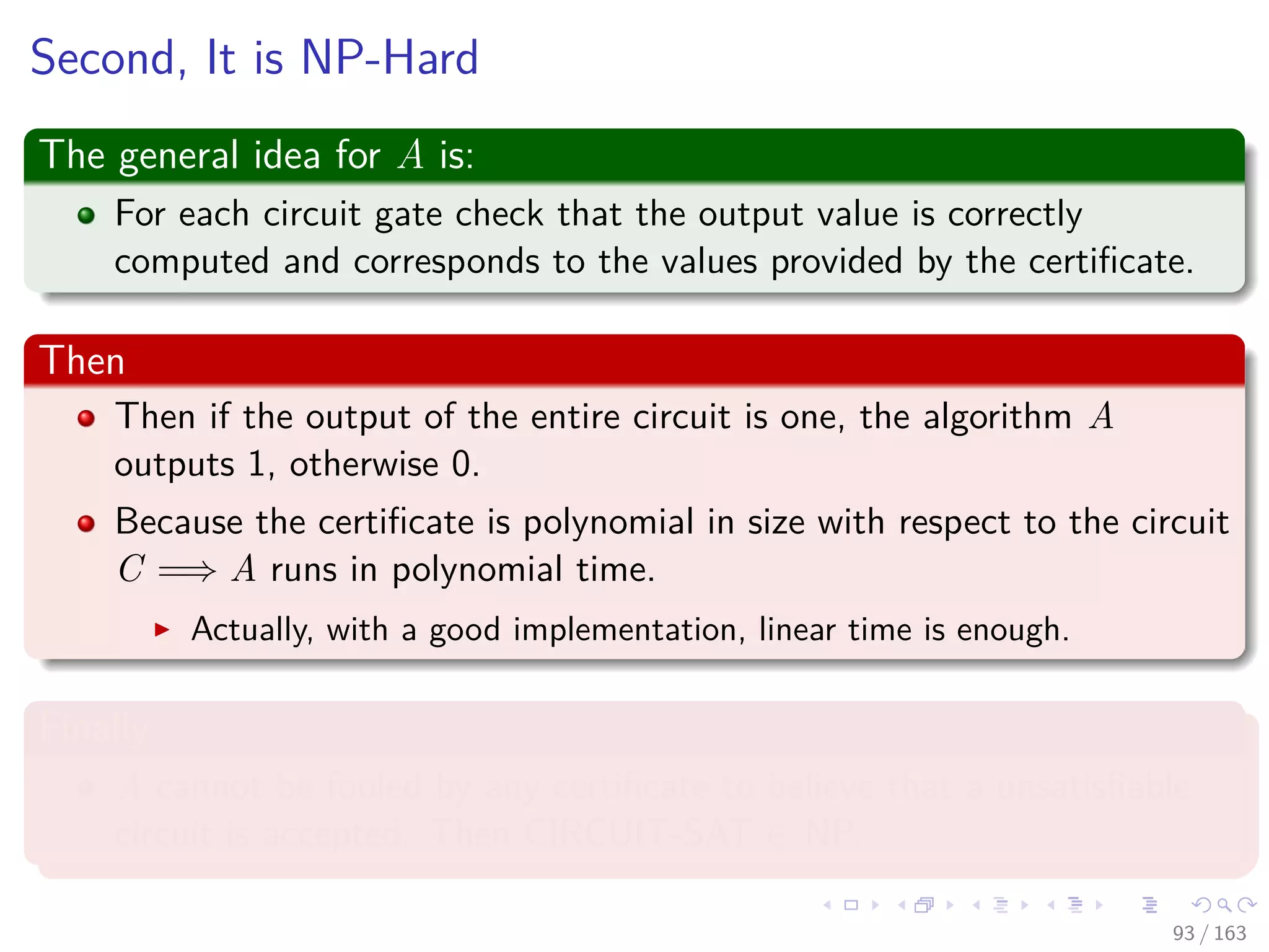
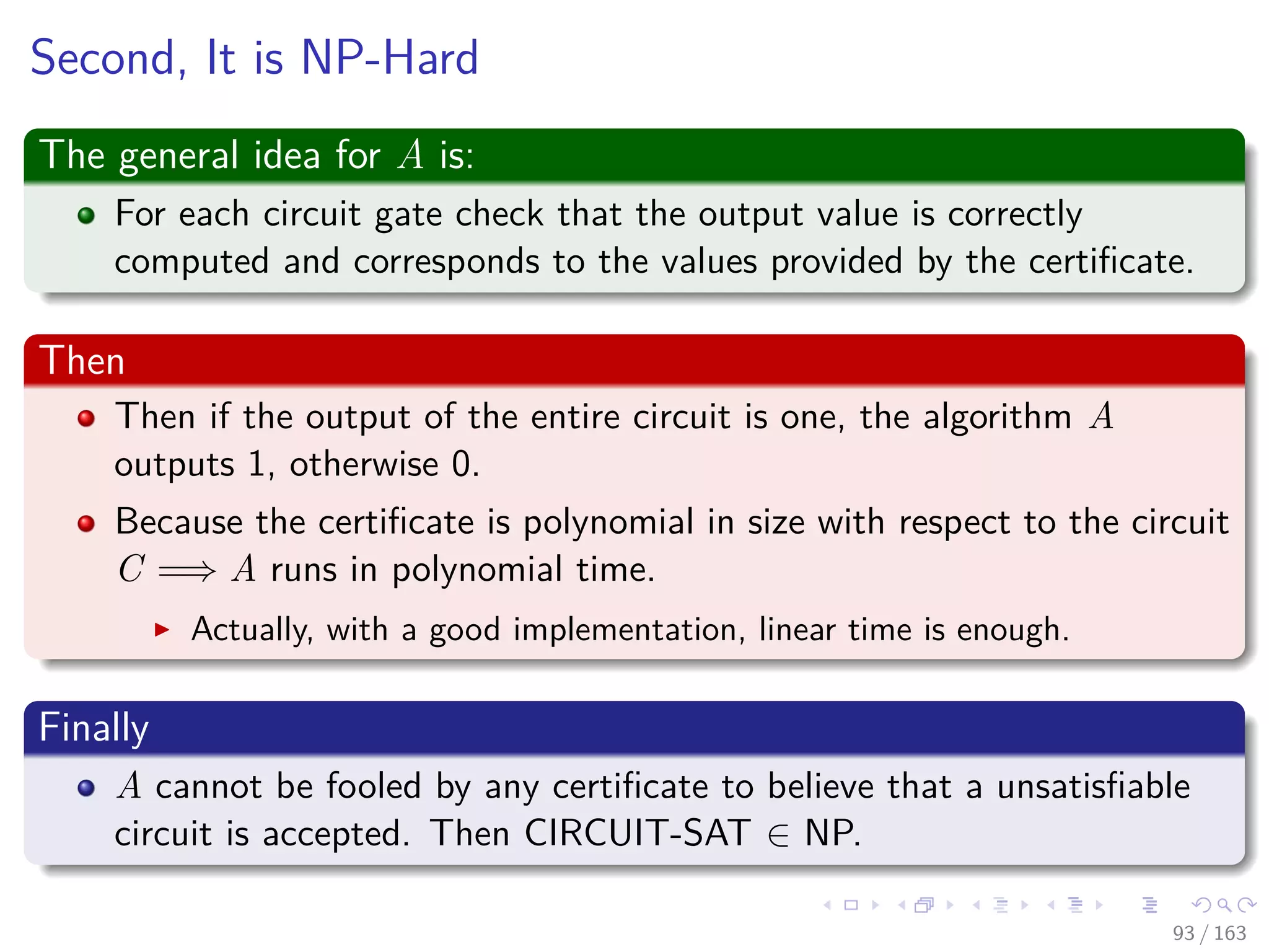
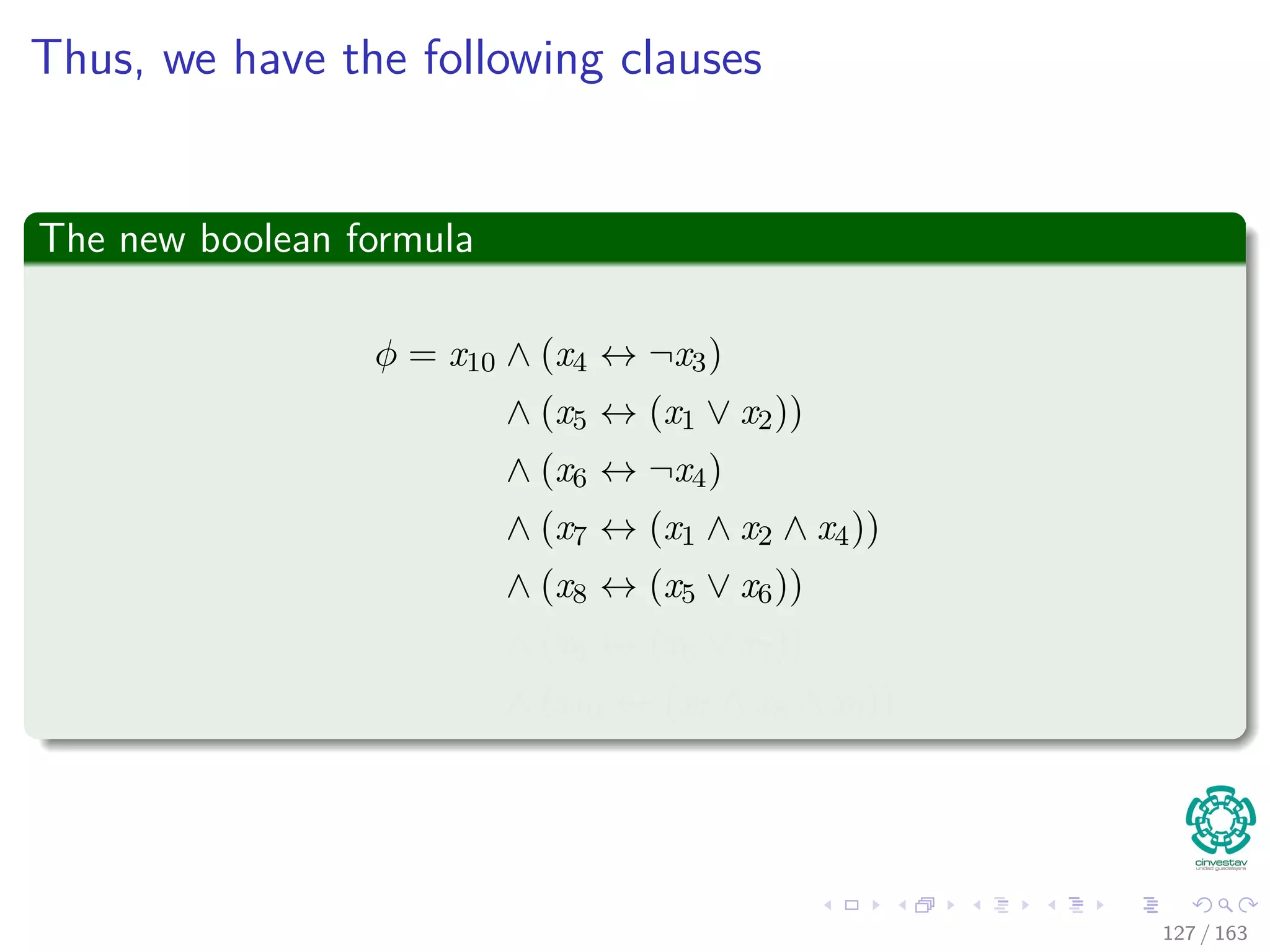
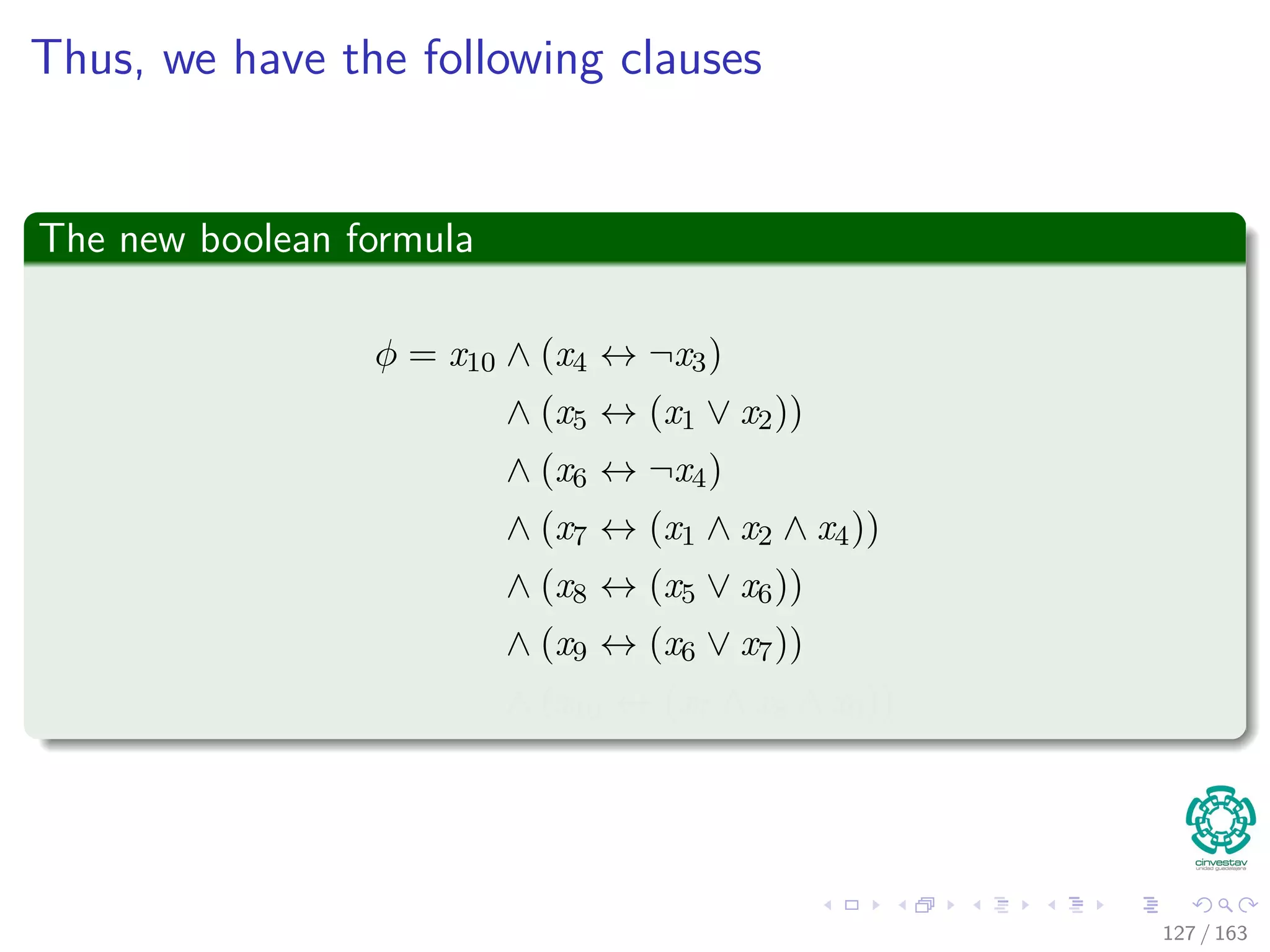
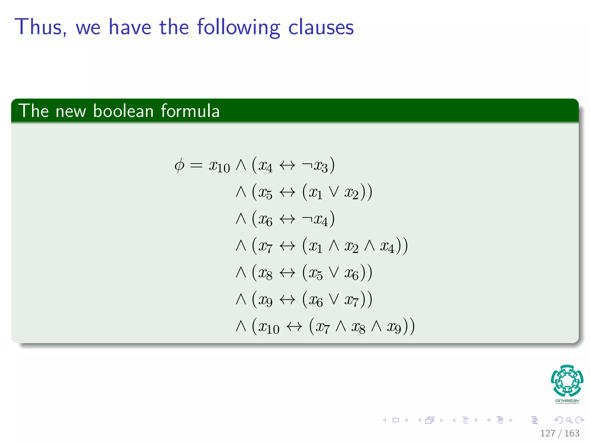
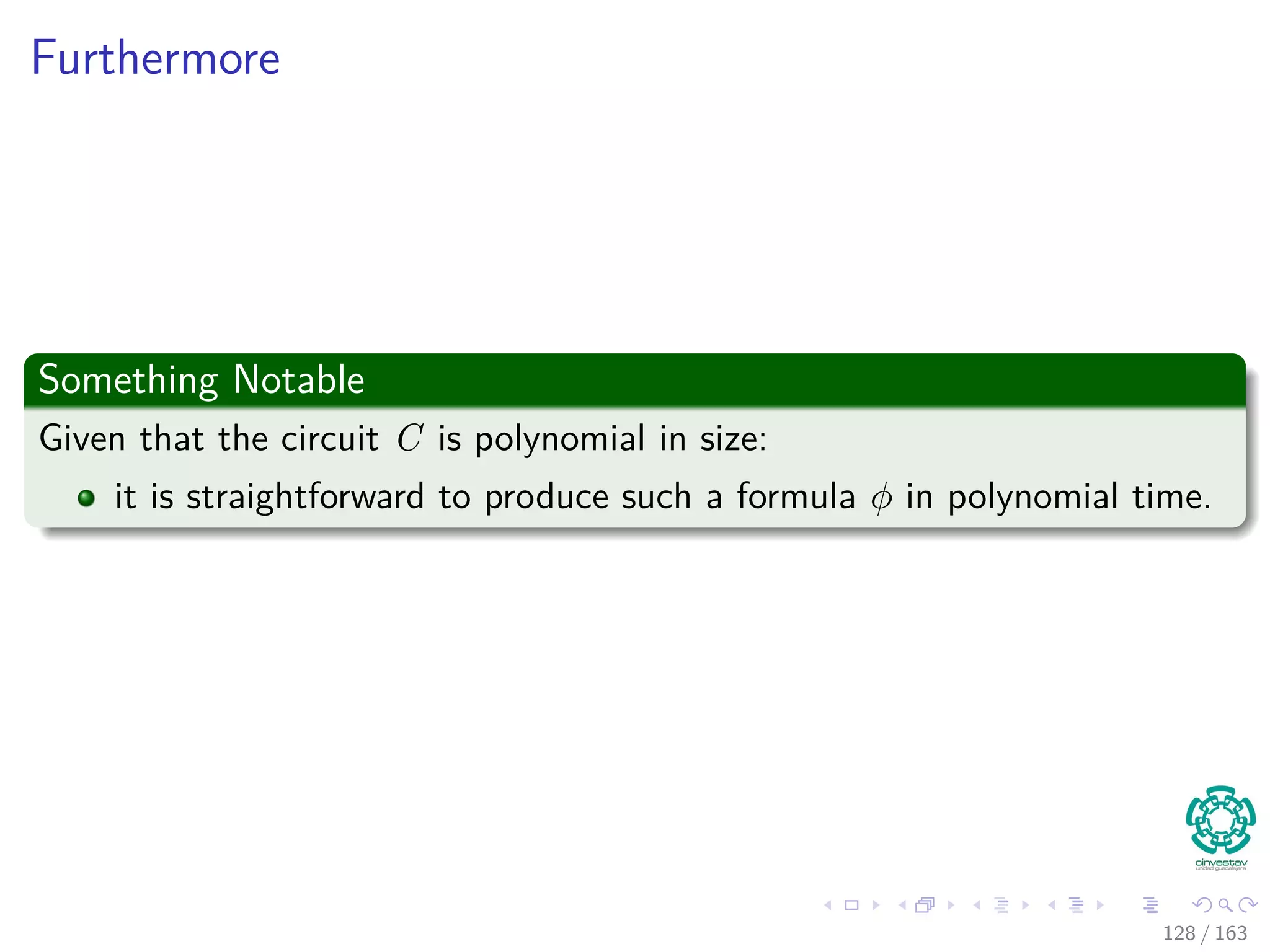
The document discusses the complexity of algorithms, particularly focusing on NP-completeness and the distinction between polynomial time (P) and non-polynomial time (NP). It outlines key concepts including polynomial time verification, reducibility, and specific NP-complete problems such as circuit satisfiability and the clique problem. It emphasizes the significance of encoding problems in a way that computational models can understand, highlighting the philosophical considerations behind classifying problems as tractable or intractable.


![Golda Meir And Arab Israeli Relations 35 Years After[1]](https://cdn.slidesharecdn.com/ss_thumbnails/golda-meir-and-arabisraeli-relations-35-years-after1-1225750179327982-9-thumbnail.jpg?width=640&height=640&fit=bounds)


![Red Star Over China (Speaker: Vincent Lee Kwun-leung) [Part 2]](https://cdn.slidesharecdn.com/ss_thumbnails/redstaroverchinapart2-140319210721-phpapp01-thumbnail.jpg?width=640&height=640&fit=bounds)