UNIT -IV DAA.pdf

1
UNIT 2 NP-COMPLETENESS AND NP-HARD
PROBLEMS
Structure Page No
2.0 Introduction
2.1 Objectives
2.2 P Vs NP-Class of Problems
2.3 Polynomial time reduction
2.4 NP-Hard and NP-Complete problem
2.4.1 Reduction
2.4.2 NP-Hard Problem
2.4.3 NP Complete Problem
2.4.4 Relation between P, NP, NP-Complete and NP-Hard
2.5 Some well-known NP-Complete Problems-definitions
2.5.1 Optimization Problems
2.5.2 Decision Problems
2.6 Techniques (Steps) for proving NP-Completeness
2.7 Proving NP-completeness (Decision problems)
2.7.1 SAT (satisfiability) Problem
2.7.2 CLIQUE Problem
2.7.3 Vertex-Cover Problem (VCP)
2.8 Summary
2.9 Solutions/Answers
2.10 Further readings
2.0 INTRODUCTION
First, let us review the topics discussed in the previous unit. In general, a class of
problems can be divided into two parts: Solvable and unsolvable problems. Solvable
problems are those for which an algorithm exist, and Unsolvable problems are those for
which algorithm does not exist such as Halting problem of Turing Machine etc. Solvable
problem can be further divided into two parts: Easy problems and Hard Problems.
Class of Problem
Solvable Unsolvable
Easy Problem (P
Class)
Hard Problem (NP
Class)
Easy Problem: Example:
Binary Search
Quicksort, Merge Sort
Dijkstra’s Algorithm
Hard Problem: Example:
Travelling Salesman Problem (TSP)
Hamiltonian Cycle Problem
0/1 Knapsack Problem

A Problem for which we know the algorithm and can be solved in polynomial time is
called a P-class (or Polynomial -Class) problem, such as Linear search, Binary Search,
Merge sort, Matrix multiplication etc.
There are some problems for which polynomial time algorithm(s) are known. Then there
are some problems for which neither we know any polynomial-time algorithm nor do
scientists believe them to exist. However, exponential time algorithms can be easily
designed for such problems. The latter class of problems is called NP (non-deterministic
polynomial). Some P and NP problems are listed in table-1.
Table-1: Examples of P-Class and NP-Class of Problems
There is a huge scope of Research related to this topic:
We Know that Linear search takes O(n) times and Binary Search takes 𝑂(𝑙𝑜𝑔𝑛)time,
Researchers are trying to search an algorithm which takes lesser time than 𝑂(𝑙𝑜𝑔𝑛),may
be 𝑂(1). We know that the lower bound of any comparison based sorting algorithm is
𝑂(𝑛𝑙𝑜𝑔𝑛),we are searching a faster algorithm than 𝑂(𝑛𝑙𝑜𝑔𝑛), may be 𝑂(𝑛).
We mentioned above it is easy to design an exponential time algorithm for any NP
problem. However, for any such problem, we ultimately want some polynomial time
algorithm. Any exponential time taking algorithm is very time-consuming algorithm as
compared to any polynomial time taking algorithm, for example:
2 , 3 , 5 , …. takes more time than any polynomial algorithms 𝑛 , 𝑛 , … . , 𝑛 .Even if, for
example, 𝑛 ∨ 𝑛 is smaller than 2 for some large value of n. Researchers from
Mathematics or Computer science are trying to write (or find) the polynomial time
algorithm for those problems for which till now no polynomial time algorithm exist. This
is a basic framework for NP-Hard and NP-Complete problems. The hierarchy of classes
of problem can be illustrated by following figure1.
P problems NP problems
Linear Search 0/1 Knapsack Prob.
Binary Search TSP
Selection Sort Sum of Subsets
Merge Sort Graph Colouring
Matrix Multiplication Hamiltonian Cycle

3
Figure-2: Hierarchy of classes of problems
Problems that can be solvable in a reasonable (polynomial) time is called tractable
problem and the intractable problems means, as they grow large, we are unable to solve
them in reasonable time. Reasonable time means we want polynomial time algorithm for
those problems. That is, on an input of size 𝑛 the worst-case running time is 𝑂 𝑛 for
some constant k.
The obvious question is “whether all problems are solvable?”. The answer is “No”. For
example, the “Halting Problem” of Turing machine is not solvable by any computer, no
matter how much time is given. Such problems are called undecidable or unsolvable
problems.
2.1 OBJECTIVES
After studying this unit, you should be able to:
 Define P, NP, NP-Complete Classes of Problems through language theoretic
framework
 Explain NP-Hard problem such as CLIQUE, Vertex-Cover Problem (VCP), 0/1
Knapsack Problem etc.
 Understanding polynomial time reduction of NP-Complete problems
 Proving NP completeness
 Explore P, NP and NP – Complete classes of problems
2.2 Definition of P and NP as Classes of Languages
Many problems from graph theory, combinatorics can be defined as language recognition
problems which require Yes/No answer for each instance of a problem. The solution to
the problem formulated as a language recognition problem can be solved by a finite

automata or any advanced theoretical machine like Turing machine ( refer to MCS-
212/Block2/Unit 2)
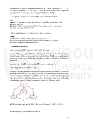
Using a formal language theory we say that the language representing a decision problem
is accepted by an algorithm A is the set of strings L = { x ∈ (0,1) ; A(x) =1}. If an
input string x is accepted by the algorithm, then A(x) = 1, and if x is rejected by the
algorithm, then A(x) = 0.
Let us introduce now important classes of languages :P, NP,NP- Complete class of
languages:
P-Class (Polynomial class):
If there exist a polynomial time algorithm for L then problem L is said to be in class P
(Polynomial Class), that is in worst case L can be solved in 𝑛 , where n is the input
size of the problem and k is positive constant.
In other word,
𝑃 = 𝐿
𝐿 𝑐𝑎𝑛 𝑏𝑒 𝑑𝑒𝑐𝑖𝑑𝑒𝑑(𝑎𝑐𝑐𝑒𝑝𝑡𝑒𝑑)𝑏𝑦 𝑑𝑒𝑡𝑒𝑟𝑚𝑖𝑛𝑖𝑠𝑡𝑖𝑐 𝑇𝑢𝑟𝑖𝑛𝑔 𝑚𝑎𝑐ℎ𝑖𝑛𝑒
(𝑎𝑙𝑔𝑜𝑟𝑖𝑡ℎ𝑚) ∈ 𝑝𝑜𝑙𝑦𝑛𝑜𝑚𝑖𝑎𝑙 𝑡𝑖𝑚𝑒
Note: Deterministic algorithm means the next step to execute after any step is unambiguously
specified. All algorithms that we encounter in real-life are of this form in which there is a
sequence of steps which are followed one after another.
Example: Binary Search, Merge sort, Matrix multiplication problem, Shortest path in a
graph (Bellman/Dijkstra’s algorithm) etc.
NP-Class (Nondeterministic Polynomial time solvable):
NP is the set of decision problems (with ‘yes’ or ‘no’ answer) that can be solved by a Non-
deterministic algorithm (or Turing Machine) in Polynomial time.
𝑁𝑃 = 𝐿
𝐿 𝑐𝑎𝑛 𝑏𝑒 𝑑𝑒𝑐𝑖𝑑𝑒𝑑 (𝑎𝑐𝑐𝑒𝑝𝑡𝑒𝑑)𝑏𝑦 𝑁𝑜𝑛𝑑𝑒𝑡𝑒𝑟𝑚𝑖𝑛𝑖𝑠𝑡𝑖𝑐 𝑇𝑢𝑟𝑖𝑛𝑔 𝑚𝑎𝑐ℎ𝑖𝑛𝑒
(𝑎𝑙𝑔𝑜𝑟𝑖𝑡ℎ𝑚) ∈ 𝑝𝑜𝑙𝑦𝑛𝑜𝑚𝑖𝑎𝑙 𝑡𝑖𝑚𝑒
Let us elaborate Nondeterministic algorithm (NDA). In NDA, certain steps have deliberate
ambiguity; essentially, there is a choice that is made during the runtime and the next few
steps depend on that choice. These steps are called the non-deterministic steps. It should be
noted that a non-deterministic algorithm is an abstract concept and no computer exists that
can run such algorithms.
Here is an example of an NDA:
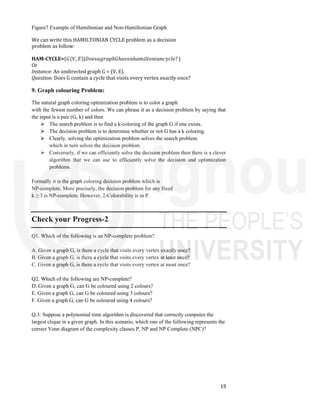
Algorithm: (Nondeterministic Linear search)
/* Input: A linear list A with n elements and a searching element 𝑥.
Output: Finds the location LOC of 𝑥in the array A (by returning an index)
or return LOC=0 to indicate 𝑥is not present in A. */
𝑁𝐷𝐿𝑆𝑒𝑎𝑟𝑐ℎ(𝐴, 𝑛, 𝑥)
{
1. [Initialize]: Set j=1 and LOC=0.
2. 𝑗 = 𝐶ℎ𝑜𝑖𝑐𝑒( ); // Nondeterministic Statement

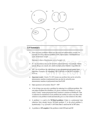
5
3. 𝑖𝑓(𝑥 = 𝐴[𝑗])
4. {
5. LOC=j
6. 𝑝𝑟𝑖𝑛𝑡𝑓
7. }
8. 𝑖𝑓(𝐿𝑂𝐶 = 0)
9. 𝑝𝑟𝑖𝑛𝑡𝑓
}
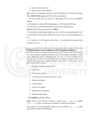
Here we assume that Line No 2 of 𝑁𝐷𝐿𝑆𝑒𝑎𝑟𝑐ℎ(𝐴, 𝑛, 𝑥) takes 1 unit of time to find the
location of searched element x (i.e. index j). So the overall time complexity of this
algorithm is 𝑂(1). Here, line no. 2 of the algorithm is nondeterministic (magical). In j is
chosen correctly, the algorithm will execute correctly, but the exact behavior can only be
known when the algorithm is running.
An DA algorithm is said to be correct if for every input value its output value is correct.
Since the actual behaviour of an NDA algorithm is only known when it is running, we
define the correctness of an NDA algorithm differently than above. An NDA algorithm is
said to be correct if for every input value there are some correct choices during the non-
deterministic steps for which the output value is correct. In the above example, there is
always some correct value of j in line no. 2 for which the algorithm is correct. Note that j
can depend on the input. For example, if A[1]=x, then j=1 is a correct choice, and if A does
not contain x, then any j is a correct choice. Hence, the above algorithm is a correct NDA
for the search problem.
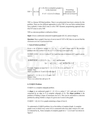
So, we can define NP class as follows:
“A nondeterministic algorithm (NDA) but takes polynomial time”. It should not difficult
to view a deterministic algorithm as also a non-deterministic algorithm that does not
make any non-deterministic choice. Thus, if there exists a DA for a problem, then the
same algorithm can also be thought of as an NDA; what this means is that if a DA exists
for a problem, then an NDA also exists for a problem. Answer to to the converse question
is not always known. Further, if the DA algorithm is polynomial-time then the NDA
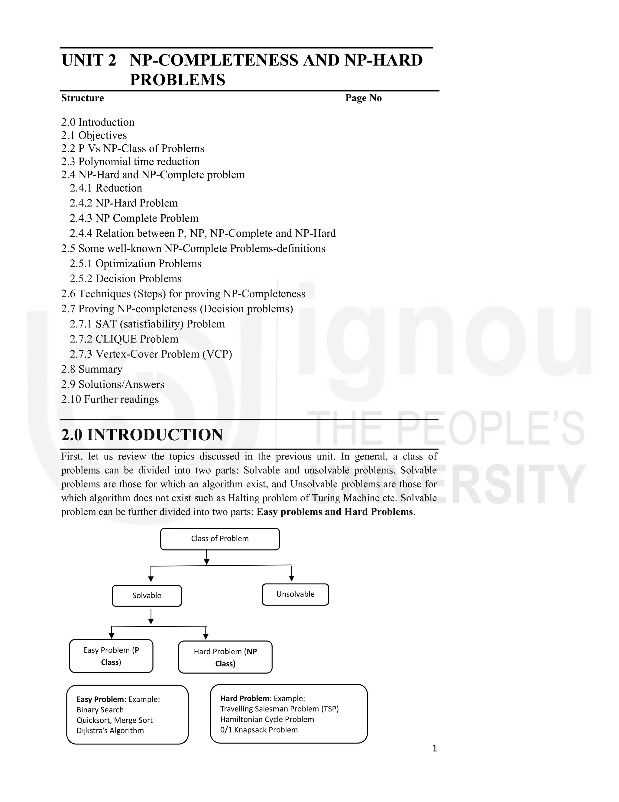
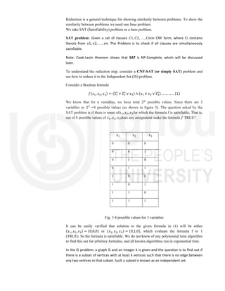
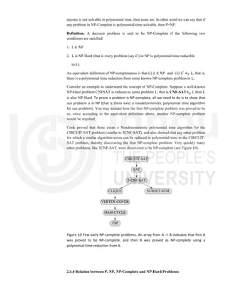
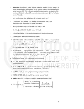
algorithm is also polynomial-time. So, we can say the following relationship hold
between P and NP class of problem.
Fig.2: Relationship between P and NP class of problem
NP
P
𝑃 ⊆ 𝑁𝑃 ……… (1)

A central question in algorithm design is the P=NP question. We discussed above that if a
problem has a polynomial time DA then it has a (trivial) polynomial-time NDA. The
P=NP question asks the converse direction. Currently we know many problems for which
there are polynomial time NDA. The question asks whether a polynomial-time NDA can
be always converted to a polynomial-time DA. This is effectively asking whether the
non-deterministic choices made by an NDA algorithm can be completely eliminated,
maybe at the cost of a slight polynomial increase in the running time. The scientist
community believes that the answer is no, i.e., P is not equal to NP, in other words, there
are NP problems which cannot be solved in polynomial time. However, the exact answer
is not known even after several decades of research.
2.3 Polynomial time Reduction
In general, any new problem requires a new algorithm. But often we can solve a problem
X using a known algorithm for a related problem Y. That is, we can reduce X to Y in the
following informal sense: A given instance x of X is translated to a suitable instance y of
Y, so that we can use the available algorithm for Y. Eventually the result of this
computation on y is translated back, so that we get the desired result for x. Let us
consider an example to understand the concept of a reduction step.
Suppose we want an algorithm for multiplying two integers, and there is already an
efficient algorithm available that can compute the square of an integer. It needs S(n) time
for an integer of n digits. Can we somehow use it to multiply arbitrary integers a, b
efficiently, without developing a multiplication algorithm? Certainly, squaring and
multiplication are related problems. More precisely, we can use the identity 𝑎𝑏 =
( ) ( )
. We only have to add and subtract the factors in O(n) time, apply our
squaring algorithm in S(n) time, and divide the result by 4, which can be easily done in
O(n) time, since the divisor is a constant. Thus, we have reduced multiplication (problem
X) to squaring (problem Y) as follows. We have taken an instance of X (factors a, b),
transformed it quickly into some instances of Y (namely 𝑎 + 𝑏 and 𝑎 − 𝑏), solved these
instances of Y by the given squaring algorithm, and finally applied another fast
manipulation on the results (addition, division by 4) to get the solution 𝑎𝑏 to the instance
of problem X. It is essential that not only a fast algorithm for Y is available, but the
transformations are fast as well.
There are two different purposes of reductions:
1. Solving a problem X with help of an already existing algorithm for a different problem
Y.
2. Showing that a problem Y is at least as difficult as another problem X.
Note that (1) is of immediate practical value, and even usual business: Ready-to-use
implementations of standard algorithms exist in software packages and algorithm
libraries. One can just apply them as black boxes, using their interfaces only, without
caring about their internal details. This is nothing but a reduction!
Point (2) gives us a way to classify problems by their algorithmic complexity. We can
compare the difficulty of two problems without knowing their “absolute” time
complexity. If Y is at least as difficult as X, then research on improved algorithms should
first concentrate on problem X.

7
Reductions-Formal definition:
Reduction is a general technique for showing similarity between problems. To show the
similarity between problems we need one base problem. A procedure which is used to
show the relationship (or similarity) between problems is called Reduction step, and
symbolically can be written as
𝐴 ≼ 𝐵
The meaning of the above statement is “problem A is polynomial time reducible to
problem B” and if there exist a polynomial time algorithm for problem A then problem B
can also have polynomial time algorithm. Here problem A is taken as a base problem
We define a reduction for decision problems X, Y as follows: We say that X is reducible
to Y in t(n) time, if we can compute in t(n) time, for any given x with |x| = n, an instance
y = f(x) of Y such that the answer to x is Yes if and only if the answer to y is Yes. If the
time t(n) needed for the reduction is bounded by a polynomial in n, we say that X is
polynomial-time reducible to Y.
Let us understand the concept of reduction using mathematical description. Suppose that
there are two problems, A and B. You know (or you strongly believe at least) that it is
impossible to solve problem A in polynomial time. You want to prove that B cannot be
solved in polynomial time. How would you do this?
We want to show that
(𝐴 ∉ 𝑃) ⇒ (𝐵 ∉ 𝑃) ----- (2)
To prove (2), we could prove the contrapositive
(𝐵 ∈ 𝑃) ⇒ (𝐴 ∈ 𝑃) [Note: (𝑄 → 𝑃is the contrapositive of 𝑃 → 𝑄]
In other words, to show that B is not solvable in polynomial time, we will suppose that
there is an algorithm that solves B in polynomial time, and then derive a contradiction by
showing that A can be solved in polynomial time.
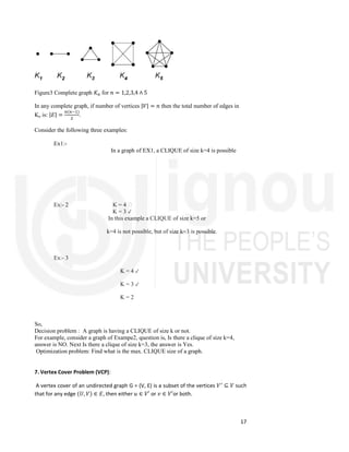
How do we do this? Suppose that we have a subroutine that can solve any instance of
problem B in polynomial time. Then all we need to do is to show that we can use this
subroutine to solve problem A in polynomial time. Thus we have “reduced” problem A to
problem B.
It is important to note here that this supposed subroutine is really a fantasy. We know (or
strongly believe) that A cannot be solved in polynomial time, thus we are essentially
proving that the subroutine cannot exist, implying that B cannot be solved in polynomial
time.
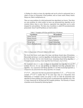
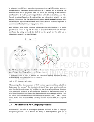
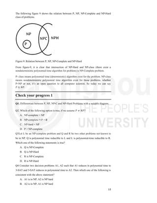
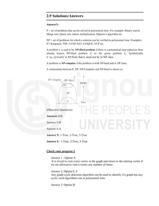
Figure 7 Reduction step of problem A to problem B
A problem A can be polynomially reduced to a problem B if there exists a polynomial-
time computable function f that converts an instance α of A into an instance β of B.
Polynomial-time algorithm to decide A
instance a
of A
instance B
of B
polynomial-time
reduction algorithm
polynomial-time
algorithm to decide B
yes
no
yes
no

Reduction is a general technique for showing similarity between problems. To show the
similarity between problems we need one base problem.
We take SAT (Satisfiability) problem as a base problem.
SAT problem: Given a set of clauses 𝐶1, 𝐶2, . . . , 𝐶𝑚in CNF form, where Ci contains
literals from 𝑥1, 𝑥2, . . . , 𝑥𝑛. The Problem is to check if all clauses are simultaneously
satisfiable.
Note: Cook-Levin theorem shows that SAT is NP-Complete, which will be discussed
later.
To understand the reduction step, consider a CNF-SAT (or simply SAT) problem and
see how to reduce it to the Independent Set (IS) problem.
Consider a Boolean formula
𝑓(𝑥 , 𝑥 , 𝑥 ) = (𝑥 ∨ 𝑥 ∨ 𝑥 ) ∧ (𝑥 ∨ 𝑥 ∨ 𝑥 ) … … … . . (1)
We know that for n variables, we have total 2 possible values. Since there are 3
variables so 2 =8 possible values (as shown in figure 3). The question asked by the
SAT problem is if there is some of𝑥 , 𝑥 , 𝑥 for which the formula f is satisfiable, That is,
out of 8 possible values of 𝑥 , 𝑥 , 𝑥 does any assignment make the formula 𝑓 TRUE?
𝑥 𝑥 𝑥
0 0 0
0 0 1
0 1 0
0 1 1
1 0 0
1 0 1
1 1 0
1 1 1
Fig. 3 8 possible values for 3 variables
It can be easily verified that solution to the given formula in (1) will be either
(𝑥 , 𝑥 , 𝑥 ) = (0,0,0) or (𝑥 , 𝑥 , 𝑥 ) = (0,1,0), which evaluate the formula f to 1
(TRUE). So the formula is satisfiable. We do not know of any polynomial time algorithm
to find this out for arbitrary formulas, and all known algorithms run in exponential time.
In the IS problem, a graph G and an integer k is given and the question is to find out if
there is a subset of vertices with at least k vertices such that there is no edge between
any two vertices in that subset. Such a subset is known as an independent set.

9
A reduction from SAT to IS is an algorithm that converts any SAT instance, which is a
Boolean formula (denoted f), to an IS instance, i.e., a graph G and an integer k. The
reduction must run in polynomial time and ensure the following: If the formula is
satisfiable then G must have an independent set with at least k vertices. And if the
formula is not satisfiable then G must not have any independent set with k or more
vertices. The catch is that the reduction must do the above without finding out if f is
satisfiable (the requirement should be obvious since there is no known algorithm to
determine satisfiability that runs in polynomial time).
Even though it may appear surprising how to perform the conversion, it is indeed
possible as is shown in Fig. 3.9. It is easy to check that the formula on the left is
satisfiable (by setting x1=1, x2=0,x3=1,x4=0) and the graph on the right has an
independent set with 3 vertices (x1,x2,x3).
Fig 3.8 The reduction algorithm from SAT to IS converts the formula on the left to the
pair of integer K and the graph shown on the right. It can be
A procedure which is used to perform this conversion between problems is called
Reduction step, and symbolically can be written as
𝑆𝐴𝑇 ≼ 0 1
⁄ 𝑘𝑛𝑎𝑝𝑠𝑎𝑐𝑘SAT <=p IS
The meaning of the above statement is “SAT problem is polynomial time reducible to
Independent Set problem”. The implication is that if there exist a polynomial time
algorithm for IS problem then SAT problem can also have polynomial time algorithm.
And furthermore, if there is no polynomial time algorithm for SAT then there cannot be
a polynomial time algorithm for IS. Here SAT problem is taken as a base problem. There
are similar reductions known between thousands of problems, like CLIQUE, Sum-of
subset, Vertex cover problem (VCP), Travelling salesman problem (TSP), 0/1-Knapsack,
etc.
2.4 NP-Hard and NP-Complete problems
In some books, NP-Hard or NP-Complete problems are stated in terms of language-
recognition problems. This is because the theory of NP-Completeness grew out of
X1 X2
X3
X1 X2
X3
X1
X2
X3
(X X X )⋀
( X X X )⋀
(X X X )
3SAT
K=3
f → f ’

automata and formal language theory. Here we will not be using this approach to define
these problems, but you should be aware that if you look in the book, it will often
describe NP-Complete problems as languages.
In theoretical computer science, the classification and complexity of common problem
definitions have two major sets; P which is “Polynomial” time and NP which “Non-
deterministic Polynomial” time. There are also NP-Hard and NP-Complete sets, which
we use to express more sophisticated problems. In the case of rating from easy to hard,
we might label these as “easy”, “medium”, “hard”, and finally “hardest”:
 𝐸𝑎𝑠𝑦 → 𝑃
 𝑀𝑒𝑑𝑖𝑢𝑚 → 𝑁𝑃
 𝐻𝑎𝑟𝑑 → 𝑁𝑃 − 𝐶𝑜𝑚𝑝𝑙𝑒𝑡𝑒
 𝐻𝑎𝑟𝑑𝑒𝑠𝑡 → 𝑁𝑃 − 𝐻𝑎𝑟𝑑
The following figure 6 shows a relationship between P, NP, NP-C and NP-Hard
problems:
Figure 6: Relationship between P, NP and NP-Complete and NP-Hard
Using the diagram, we assume that P and NP are not the same set, or, in other words, we
assume that 𝑃 ≠ 𝑁𝑃. Another interesting result from the diagram is that there is an
overlap between NP and NP-Hard problem. We call this NP-Complete problem
(problem belongs to both NP and NP-Hard sets).
NP-Complete problems are the “hardest” problems to solve among all NP problems, in
that if one of them can be solved in polynomial time then every problem in NP can be
solved in polynomial time. This is where the concept of reduction comes in. There may
be even harder problems to solve that are not in the class of NP, called NP-Hard
problems.
The study of NP Completeness is important: the most cited reference in all of Computer
Science is Garey & Johnson’s (1979) book Computers and Intractability: A Guide to the
Theory of NP-Completeness. (A text book is the second most cited reference in
Computer Science!).
In 1979 Garey & Johnson wrote, “The question of whether or not the NP-complete
problems are intractable is now considered to be one of the foremost open questions of
contemporary mathematics and computer science.”
NP
P
NP-Hard
Hardest
Hard
Medium
Easy
NP-Complete

11
Over 30 years later, in spite of a million-dollar prize offer and intensive study by many of
the best minds in computer science, this is still true: No one has been able to either
 Prove that there are problems in NP that cannot be solved in polynomial time
(which would mean P ≠NP), or
 Find a polynomial time solution for a single NP Complete Problem (which would
mean P=NP).
Although either alternative is possible, most computer scientists believe that P ≠ NP
Now, to understand the concept of NP-Hard problem, let us consider by the following
example.
CNF-SAT problem is well known NP-Hard problem (a base problem to prove other
problems are NP-Hard) and let us call all the other exponential time taking problems (0/1
knapsack, TSP, VCP, Hamiltonian cycle etc.) as a hard problem. We can say that if all
these hard problems are related to CNF-SAT problem and if CNF-SAT is solved (in
polynomial time) then all these hard problems can also be solved in polynomial time.
2.4.2 NP-Hard Problem
Definition: A problem L is said to be NP-Hard problem if there is a polynomial time
reduction from already known NP-Hard problem 𝐿 to the given problem L.
Symbolically 𝐿 ≼ 𝐿𝑓𝑜𝑟𝑎𝑙𝑙𝐿 ∈ 𝑁𝑃
Note that L need not be in NP class.
Let us consider an example to understand the concept of NP-Hard. We have already seen
a CNF-SAT problem is polynomial time reducible to 0/1 knapsack problem, and denoted
as CNF-SAT≼ 0 1
⁄ 𝑘𝑛𝑎𝑝𝑠𝑎𝑐𝑘 ---(1)
Here CNF-SAT is already known NP-Hard problem and this known NP-hard problem is
polynomial time reduces to given problem L (i.e., 0/1 knapsack problem). By writing
CNF-SAT≼ 0 1
⁄ 𝑘𝑛𝑎𝑝𝑠𝑎𝑐𝑘 means that “if 0/1 knapsack problem is solvable in
polynomial time, then so is 3CNF-SAT problem, which also means that, if 3CNF-SAT is
not solvable in polynomial time, then the 0/1 knapsack problem can't be solved in
polynomial time either.”
In other word, here we show that any instance (say 𝐼 ) or formula of CNF-SAT problem
is converted into a 0/1 knapsack problem (say instance 𝐼 ) and we can say that if 0/1
knapsack problem is solved in polynomial time by using an algorithm A then the same
algorithm A can also be used to solve CNF-SAT problem in polynomial time. Note that
reduction (or conversion) step takes polynomial time.
2.4.3 NP-Complete Problem
NP-Complete problems are the “hardest” problems to solve among all NP problems. The
set of NP-complete problems are all problems in the complexity class NP, for which it is
known that if anyone is solvable in polynomial time, then they all are, and conversely, if

anyone is not solvable in polynomial time, then none are. In other word we can say that if
any problem in NP-Complete is polynomial-time solvable, then P=NP.
Definition: A decision problem is said to be NP-Complete if the following two
conditions are satisfied:
1. 𝐿 ∈ 𝑁𝑃
2. L is NP Hard (that is every problem (say 𝐿 ) in NP is polynomial-time reducible
to L).
An equivalent definition of NP-completeness is that (i) 𝐿 ∈ 𝑁𝑃 and (ii) 𝐿 ≼ 𝐿, that is,
there is a polynomial time reduction from some known NP-complete problem to L.
Consider an example to understand the concept of NP-Complete. Suppose a well-known
NP-Hard problem CNFSAT is reduces to some problem L, that is CNF-SAT≼ 𝐿 then L
is also NP-Hard. To prove a problem is NP-complete, all we need to do is to show that
our problem is in NP (that is there exist a nondeterministic polynomial time algorithm
for our problem). You may wonder how the first NP-complete problem was proved to be
so, since according to the equivalent definition above, another NP-complete problem
would be required.
Cook proved that there exists a Nondeterministic polynomial time algorithm for the
CIRCUIT-SAT problem (similar to 3CNF-SAT), and also showed that any other problem
for which a similar algorithm exists can be reduced in polynomial-time to the CIRCUIT-
SAT problem, thereby discovering the first NP-complete problem. Very quickly many
other problems, like 3CNF-SAT, were discovered to be NP-complete (see Figure 10).
Figure 10 Few early NP-complete problems. An array from A -> B indicates that first A
was proved to be NP-complete, and then B was proved as NP-complete using a
polynomial-time reduction from A.
2.4.4 Relation between P, NP, NP-Complete and NP-Hard Problems:

13
The following figure 9 shows the relation between P, NP, NP-Complete and NP-Hard
class of problems.
Figure 9: Relation between P, NP, NP-Complete and NP-Hard
From figure-9, it is clear that intersection of NP-Hard and NP-class (there exist a
nondeterministic polynomial time algorithm for problem) is NP-Complete problem.
P- class means polynomial time (deterministic) algorithm exist for the problem. NP-class
means nondeterministic polynomial time algorithm exist for those problems. whether
P=NP or not, it’s an open question to all computer scientist. So today we can say
𝑃 ⊆ 𝑁𝑃.
Check your progress 1
Q1. Differentiate between P, NP, NP-C and NP-Hard Problems with a suitable diagram.
Q2. Which of the following option is true, if we assume 𝑃 ≠ 𝑁𝑃?
A. NP-complete = NP
B. NP-complete ∩ P = ∅
C. NP-hard = NP
D. P = NP-complete
Q3Let L be an NP-complete problem and Q and R be two other problems not known to
be in NP. Q is polynomial time reducible to L and L is polynomial-time reducible to R.
Which one of the following statements is true?
A. Q is NP-Complete
B. Q is NP-Hard
C. R is NP-Complete
D. R is NP-Hard
Q4 Consider two decision problems A1, A2 such that A1 reduces in polynomial time to
3-SAT and 3-SAT reduces in polynomial time to A2. Then which one of the following is
consistent with the above statement?
A. A1 is in NP, A2 is NP hard
B. A2 is in NP, A1 is NP hard

C. Both A1 and A2 are in NP
D. Both A1 and A2 are in NP hard
Q5: Consider the following statements about NP-Complete and NP-Hard problems.
Write TRUE/FALSE against each of the following statements
1. The first problem that was proved as NP-complete was the circuit satisfiability
problem.
2. NP-complete is a subset of NP Hard problems, i.e. NP-Complete⊆NP-Hard.
3. SAT problem is well-known NP-Hard as well as NP-Complete problem.
Q6 Which of the following statements are TRUE?
1. The problem of determining whether there exists a cycle in an undirected graph is in P.
2. The problem of determining whether there exists a cycle in an undirected graph is in
NP.
3. If a problem A is NP-Complete, there exists a non-deterministic polynomial time
algorithm to solve A.
2.5 Definitions of some well-known NP-Complete problems
We have seen many problems that can be solved in polynomial time such as Binary
search, Merge sort, matrix multiplication etc. The class of all these problems are so
solvable are in P-Class. The following are some well-known problems that are NP-
complete when expressed as decision problem (with ‘YES’ or ‘NO’ answer). In the
previous unit we have defined
1. Boolean satisfiability problem (SAT)
2. 3-CNF SAT
3. 0/1 Knapsack problem.
4. Travelling salesman problem (decision version)
5. Subset sum problem.
6. Clique problem.
7. Vertex cover problem.
8. Hamiltonian cycle problem.
9. Graph coloring problem
1. SAT problem is defined as follows:
Input: Given a CNF formula f having m clauses 𝐶 , 𝐶 , … … . , 𝐶 in n variables
𝑥 , 𝑥 , … … . , 𝑥 . There is no restriction on number of variables in each clause.
The problem is to find an assignment (value) to a set of variables 𝑥 , 𝑥 , … … . , 𝑥 which
satisfy all the m clauses simultaneously.

In other word, “is there an assignment of values (0 or 1) to the variables
which makes the formula f to TRUE (or 1)”?. Note that there are
(values) to the n variable so exhaustive search will take time
𝑆𝐴𝑇 = {𝑓: 𝑓 is a given Boolean formula in CNF, Is this formula
SAT:
Instance: A Boolean formula ∅consisting of variables, parentheses, and
and/or/not operators.
Question: Is there an assignment of True/False values to the variables that
makes the formula evaluate to True?
2. 3-CNF-SAT Problem: 3-CNF SAT problem is defined as follows:
3-SAT:
Instance: A CNF formula with 3 literals in each clause.
Question: Is there an assignment of True/False values to the variables
that makes the formula evaluate to True?
3. 0/1Knapsack problem:
A decision version of 0/1 knapsack problem is NP
Given a list {𝑖 , 𝑖 , … , 𝑖 }, a knapsack with capacity M
object 𝑖 has a weight 𝑤 and value 𝑣 . Can a subset of items
whose total weight is at most M and at total value is at least V?
constraints:
Maximize (the value) ∑ 𝑣 𝑥 such that ∑
4. Traveling Salesman Problem (TSP):
Given a set of cities and distance between every pair of cities, the problem is to find the
shortest possible route that visits every city exactly once and returns to the starting point.
There is a integer cost 𝐶(𝑖, 𝑗) to travel from city i to city j and t
make the tour whose total cost is minimum, where the total cost is the sum of individual
costs along the edges of the tour. For example, consider the following graph:
A TSP tour in the graph is A-B-D-C-A. The cost of the tour is 10
In formal language, TSP problem is defined as:
15
In other word, “is there an assignment of values (0 or 1) to the variables 𝑥 , 𝑥 , … … . , 𝑥
la f to TRUE (or 1)”?. Note that there are 2 possible assignments
(values) to the n variable so exhaustive search will take time 𝑂(2 ).
is a given Boolean formula in CNF, Is this formula 𝑓satisfiable?}
consisting of variables, parentheses, and
: Is there an assignment of True/False values to the variables that
CNF SAT problem is defined as follows:
A CNF formula with 3 literals in each clause.
Is there an assignment of True/False values to the variables
that makes the formula evaluate to True?
A decision version of 0/1 knapsack problem is NP-complete.
a knapsack with capacity M and a desired value V . Each
. Can a subset of items 𝑋 ⊆ {𝑖 , 𝑖 , … , 𝑖 } be picked
whose total weight is at most M and at total value is at least V? that satisfy the following
𝑤 𝑥 ≤ 𝑀 and 𝑥 ∈ {0,1}
Given a set of cities and distance between every pair of cities, the problem is to find the
shortest possible route that visits every city exactly once and returns to the starting point.
to travel from city i to city j and the salesman wishes to
make the tour whose total cost is minimum, where the total cost is the sum of individual
costs along the edges of the tour. For example, consider the following graph:
A. The cost of the tour is 10+25+30+15=80
In formal language, TSP problem is defined as:

𝑇𝑆𝑃 =
⎩
⎪
⎨
⎪
⎧
⟨𝐺, 𝐶, 𝑘⟩
𝐺 = (𝑉, 𝐸)𝑖𝑠 𝑎 𝑐𝑜𝑚𝑝𝑙𝑒𝑡𝑒 𝑔𝑟𝑎𝑝ℎ, 𝐶
𝑖𝑠 𝑡ℎ𝑒 𝑓𝑢𝑛𝑐𝑡𝑖𝑜𝑛
𝑉 × 𝑉 → 𝑍, 𝑘 ∈ 𝑍 ∧ 𝐺ℎ𝑎𝑠𝑎
𝑇𝑟𝑎𝑣𝑒𝑙𝑙𝑖𝑛𝑔
𝑠𝑎𝑙𝑒𝑎𝑚𝑎𝑛 𝑡𝑜𝑢𝑟
𝑤𝑖𝑡ℎ 𝑐𝑜𝑠𝑡 𝑎𝑡 𝑚𝑜𝑠𝑡 𝑘
⎭
⎪
⎬
⎪
⎫
TSP is a famous NP-Hard problem. There is no polynomial time know solution for this
problem. There are few different approaches to solve TSP. if we use Naïve method (brute
force method), it takes 𝜃(𝑛!) time to solve TSP. Dynamic programming approach takes
𝑂(𝑛 2 ) time to solve TSP.
TSP as a decision problem is defined as follow:
Input: Given a undirected connected weighted graph 𝐺(𝑉, 𝐸), and an integer k.
Question: Does a graph G has tour of cost at most 𝑘? If P ≠ NP, then we can not find the
minimum-cost tour in polynomial time.
5. Sum-of-Subset problem:
Given a set of positive integer S = {x1, x2, ..., xn} and a target sum K, the decision
problem asks for a subset 𝑆 of S(𝑖. 𝑒. 𝑆 ⊆ 𝑆) having a sum equal to K.
SUBSET_SUM = {⟨S, k⟩: ∃ subset 𝑆 ⊆ 𝑆 such that sum of elements of 𝑆 equal to given
sum k}.
Example: Suppose an input Set S = {2, 3, 5, 8, 10, 4, 6}, and Sum k = 9
Output: True
There is a subset (4, 5) and (3,6) with sum 9.
Input set S = {3, 34, 4, 12, 5, 2}, sum = 30
Output: False
There is no subset that add up to 30
6. CLIQUE Problem:
CLIQUE is a complete subgraph problem.
A clique in an undirected graph G = (V, E) is a subset V’ ⊆V, each pair of which is
connected by an edge in E (a complete subgraph of G). The clique problem is the
problem of finding a clique of maximum size in G. This can be converted to a decision
problem by asking whether a clique of a given size k exists in the graph:
CLIQUE = {⟨G, k⟩: G is a graph containing a clique of size k}
To understand a CLIQUE problem, let us first define a Complete Graph. A complete
graph is one in which every vertex of G is connected with every other vertices of G, and
it is denoted by 𝐾 . Some examples of complete graph for n = 1,2,3,4 and 5 are shown in
figure-3

17
Figure3 Complete graph 𝐾 for 𝑛 = 1,2,3,4 ∧ 5
In any complete graph, if number of vertices |𝑉| = 𝑛 then the total number of edges in
Kn is: |𝐸| =
( )
.
Consider the following three examples:
Ex1:-
In a graph of EX1, a CLIQUE of size k=4 is possible
Ex:- 2 K = 4 ╳
K = 3 ✓
In this example a CLIQUE of size k=5 or
k=4 is not possible, but of size k=3 is possible.
Ex:- 3
K = 4 ✓
K = 3 ✓
K = 2
So,
Decision problem : A graph is having a CLIQUE of size k or not.
For example, consider a graph of Exampe2, question is, Is there a clique of size k=4,
answer is NO. Next Is there a clique of size k=3, the answer is Yes.
Optimization problem: Find what is the max. CLIQUE size of a graph.
7. Vertex Cover Problem (VCP):
A vertex cover of an undirected graph G = (V, E) is a subset of the vertices 𝑉 ⊆ 𝑉 such
that for any edge (𝑈, 𝑉) ∈ 𝐸, then either 𝑢 ∈ 𝑉′ or 𝑣 ∈ 𝑉′or both.

In other word, a vertex cover is a subset of all of the vertices of a graph such that every
edge in the graph is “covered” or incident to at least one vertex in the vertex cover subset.
The size of the vertex cover, then, is simply the number of vertices in the vertex cover
subset. For Example, the vertex cover set for the following graph, as shown in figure-5 is
{𝑎, 𝑐, 𝑑, 𝑒} ∨ {𝑎, 𝑏, 𝑑, 𝑒}.
Figure-5: Vertex Cover for G is {𝑎, 𝑐, 𝑑, 𝑒} ∨ {𝑎, 𝑏, 𝑑, 𝑒}
Vertex Cover as a decision problem
The problem VERTEX COVER, stated as a decision problem, is to determine whether a
given graph 𝐺(𝑉, 𝐸) with |V|=n, has a vertex cover of size k, where 𝑘 ≤ 𝑛.
VERTEX-COVER = {⟨𝐺, 𝑘⟩: graph G has a vertex cover of size k}
VERTEX COVER:
Instance: A graph G and an integer K.
Question: Is there a set of K vertices in G that touches each edge at least
once?
So, the input to VERTEX COVER is a graph G and an integer k. The algorithm returns
either a certificate/witness, or “no such vertex cover exists”.
8. Hamiltonian Cycle problem:
A Hamiltonian Cycle of an undirected graph 𝐺(𝑉, 𝐸) is a simple cycle that passes
through all the vertices of the graph G exactly once. For example, the following graph as
shown in figure, contains a cycle 𝑎 − 𝑏 − 𝑐 − 𝑓 − 𝑑 − 𝑒 − 𝑎 that visits each vertex
exactly once. Therefore, the cycle is a Hamiltonian cycle. On the other hand, in the
second graph, there exists a cycle in the graph that visits all vertices, 𝑎 − 𝑏 − 𝑑 − 𝑐 −
𝑓 − 𝑑 − 𝑒 − 𝑎 but vertex d appears twice in the cycle. Thus, it is not a Hamiltonian cycle
f
d
e
c
b
a
d
b
a
c
f
e
a
b
e
d
c
f
Hamiltonian Graph Non Hamiltonian

19
Figure7 Example of Hamiltonian and Non-Hamiltonian Graph
We can write this HAMILTONIAN CYCLE problem as a decision
problem as follow:
HAM-CYCLE={𝐺(𝑉, 𝐸}|𝐷𝑜𝑒𝑠𝑎𝑔𝑟𝑎𝑝ℎ𝐺ℎ𝑎𝑣𝑒𝑎ℎ𝑎𝑚𝑖𝑙𝑡𝑜𝑛𝑖𝑎𝑛𝑐𝑦𝑐𝑙𝑒? }
Or
Instance: An undirected graph G = (V, E).
Question: Does G contain a cycle that visits every vertex exactly once?
9. Graph colouring Problem:
The natural graph coloring optimization problem is to color a graph
with the fewest number of colors. We can phrase it as a decision problem by saying that
the input is a pair (G, k) and then
 The search problem is to find a k-coloring of the graph G if one exists.
 The decision problem is to determine whether or not G has a k coloring.
 Clearly, solving the optimization problem solves the search problem
which in turn solves the decision problem.
 Conversely, if we can efficiently solve the decision problem then there is a clever
algorithm that we can use to efficiently solve the decision and optimization
problems.
Formally it is the graph coloring decision problem which is
NP-complete. More precisely, the decision problem for any fixed
k ≥ 3 is NP-complete. However, 2-Colorability is in P.
Check your Progress-2
Q1. Which of the following is an NP-complete problem?
A. Given a graph G, is there a cycle that visits every vertex exactly once?
B. Given a graph G, is there a cycle that visits every vertex at least once?
C. Given a graph G, is there a cycle that visits every vertex at most once?
Q2. Which of the following are NP-complete?
D. Given a graph G, can G be coloured using 2 colours?
E. Given a graph G, can G be coloured using 3 colours?
F. Given a graph G, can G be coloured using 4 colours?
Q.3: Suppose a polynomial time algorithm is discovered that correctly computes the
largest clique in a given graph. In this scenario, which one of the following represents the
correct Venn diagram of the complexity classes P, NP and NP Complete (NPC)?

2.8 Summary
 There are many problems which have decision and optimization versions, for
example Traveling salesman problem (TSP). Optimization: find Hamiltonian
cycle of minimum weight.
Decision: is there a Hamiltonian cycle of weight ≤ 𝑘.
 P = set of problems that can be solved in polynomial time. For example: Binary
search, Merge sort, Quick sort, matrix multiplication, Dijkstra’s algorithm etc.
 NP = set of problems for which there is a non-deterministic polynomial time
algorithm. Examples: 0/1 Knapsack, TSP, CNFSAT, 3-CNF SAT, CLIQUE,
VCP etc.
 Important results: Clearly 𝑃 ⊆ 𝑁𝑃 (means any problem that can be solved by
deterministic machine in polynomial time can also be solved by non-
deterministic machine in polynomial time) but P≠NP
 Open question to all scientist: Does P = NP?
 A lot of times you can solve a problem by reducing it to a different problem. We
can reduce Problem B to Problem A if, given a solution to Problem A, we can
easily (“easily” means polynomial time) construct a solution to Problem B. That
is reduction (or translation) of one problem into another in such a way that a fast
solution to one problem would automatically give us a fast solution to the other.
 A problem L is said to be NP-Hard problem if there is a polynomial time
reduction from already known NP-Hard problem 𝐿 to the given problem L.
Symbolically 𝐿 ≼ 𝐿𝑓𝑜𝑟𝑎𝑙𝑙𝐿 ∈ 𝑁𝑃.Note that L need not be in NP class.
 A problem is NP-complete if the problem is both NP-hard and NP.
(C)
(A) (B)
(D) P=NP=NPC
NP
P=NP
NP
NPC
P
NPC
p

21
 Reduction: A problem R can be reduced to another problem Q if any instance of
R can be rephrased to an instance of Q, the solution to which provides a solution
to the instance of R. This rephrasing is called a transformation or reduction. The
intuition behind this is that, If R reduces in polynomial time to Q, R is “no harder
to solve” than Q.
 If A is polynomial-time reducible to B, we denote this 𝐴 ≼ 𝐵
 Definition of NP-Hard and NP-Complete: If all problems 𝑅 ∈ 𝑁𝑃are
polynomial-time reducible to Q, then Q is NP-Hard.
 We say Q is NP-Complete if Q is NP-Hard and 𝑄 ∈ 𝑁𝑃
 If 𝑅 ≼ 𝑄 and R is NP-Hard, Q is also NP-Hard.
 Circuit Satisfiability (SAT) problem is the first NP-Complete problem.
 (Properties of polynomial time reductions):
 if Problem L1 is polynomial time reducible to L2 and if L2 is solvable in
polynomial time then L1 can also be solvable in Polynomial time, that is,
If 𝐿 ≼ 𝐿 and 𝐿 ∈ 𝑃 then 𝐿 ∈ 𝑃.
 2. If 𝐿 ≼ 𝐿 and 𝐿 ∈ 𝑁𝑃 then 𝐿 ∈ 𝑁𝑃
 3. If Problem L1 is polynomial time reducible to L2 and if L1 is not likely
to be solvable in polynomial time then L2 is also not likely to be solvable
in polynomial time, that is If 𝐿 ≼ 𝐿 and 𝐿 𝑃 then 𝐿 𝑃.
 Definitions of some well-known decision problems:
 𝑆𝐴𝑇 = {𝑓: 𝑓is a given Boolean formula in CNF with n variables and m clauses, Is this
formula 𝑓satisfiable?}
 3𝐶𝑁𝐹 − 𝑆𝐴𝑇 = {𝑓: 𝑓is a given Boolean formula in CNF with n variables and m
clauses and at most 3 literals per clause, Is this formula 𝑓satisfiable?}
 CLIQUE = {⟨G, k⟩: G is a graph containing a clique of size k}
 VERTEX-COVER = {⟨𝐺, 𝑘⟩: graph G has a vertex cover of size k}
 HAM-CYCLE={𝐺(𝑉, 𝐸}| Does a Graph G has a Hamiltonian Cycle?}
 𝑇𝑆𝑃 =
⎩
⎪
⎨
⎪
⎧
⟨𝐺, 𝐶, 𝑘⟩
𝐺 = (𝑉, 𝐸) 𝑖𝑠 𝑎 𝑐𝑜𝑚𝑝𝑙𝑒𝑡𝑒
𝑔𝑟𝑎𝑝ℎ, 𝐶 𝑖𝑠 𝑡ℎ𝑒 𝑓𝑢𝑛𝑐𝑡𝑖𝑜𝑛
𝑉 × 𝑉 → 𝑍, 𝑘 ∈ 𝑍 ∧ 𝐺ℎ𝑎𝑠𝑎
𝑇𝑟𝑎𝑣𝑒𝑙𝑙𝑖𝑛𝑔
𝑠𝑎𝑙𝑒𝑎𝑚𝑎𝑛 𝑡𝑜𝑢𝑟
𝑤𝑖𝑡ℎ 𝑐𝑜𝑠𝑡 𝑎𝑡 𝑚𝑜𝑠𝑡 𝑘
⎭
⎪
⎬
⎪
⎫

2.9 Solutions/Answers
Answer1:
P = set of problems that can be solved in polynomial time. For example: Binary search,
Merge sort, Quick sort, matrix multiplication, Dijkstra’s algorithm etc.
NP = set of problems for which a solution can be verified in polynomial time. Examples:
0/1 Knapsack, TSP, 3-CNF SAT, CLIQUE, VCP etc.
A problem L is said to be NP-Hard problem if there is a polynomial time reduction from
already known NP-Hard problem 𝐿 to the given problem L. Symbolically
𝐿 ≼ 𝐿𝑓𝑜𝑟𝑎𝑙𝑙𝐿 ∈ 𝑁𝑃.Note that L need not be in NP class.
A problem is NP-complete if the problem is both NP-hard and in NP class.
A relationship between P, NP, NP-Complete and NP-Hard is shown as:
(Objective Questions)
Answers 2-B
Answer 3-D
Answer 4-A
Answer 5: 1-True, 2-True, 3-True
Answer 6 : 1-True, 2-True, 3-True
Check your progress 2
Answer 1 : Option A
It is trivial to visit every vertex in the graph and return to the starting vertex if
we are allowed to visit a vertex any number of times.
Answer 2: Option E, F
Any graph cycle detection algorithm can be used to identify if a graph has any
cycle; such algorithms run in polynomial time.
Answer 3: Option D

23
2.11 FURTHER READINGS
1. Introduction to Algorithms. Thomas H. Cormen, Charles E. Leiserson,
Ronald L. Rivest, and Clifford Stein (PHI)
2. Algorithm Design, Jon Kleinberg and Eva Tardos, Pearson
3. Fundamentals of Algorithmics, G. Brassard & P. Brately: (Prentice-Hall
International, 1996).
4. Fundamental Algorithms (Second Edition), D.E. Knuth: (Narosa Publishing
House).
5. Fundamentals of Computer Algorithms, E. Horowitz & S. Sahni: (Galgotia
Publications).
6. The Design and Analysis of Algorithms, Anany Levitin: (Pearson Education,
2003).
**********************************

UNIT -IV DAA.pdf

Recommended

Recommended

More Related Content

Similar to UNIT -IV DAA.pdf

Similar to UNIT -IV DAA.pdf (20)

Recently uploaded

Recently uploaded (20)

UNIT -IV DAA.pdf