The document discusses an introduction to basic concepts in computational complexity theory presented by a PhD student. It covers definitions of algorithms, asymptotic analysis using Big O notation, and computational models including Turing machines, multi-tape Turing machines, non-deterministic Turing machines, and oracle Turing machines. It also introduces complexity classes such as P, NP, NTIME and discusses how different computational models are equivalent in computational power.


![兩個序列的分析 在 1970 年代,分子生物學家 Needleman 及 Wunsch [15] 以動態程式設計技巧 (dynamic programming) 分析了氨基酸序列的相似程度; 有趣的是,在同一時期,計算機科學家 Wagner 及 Fisher [22] 也以極相似的方式來計算兩序列間的編輯距離 (edit distance) ,而這兩個重要創作當初是在互不知情下獨立完成的。 雖然分子生物學家看的是兩序列的相似程度,而計算機科學家看的是兩序列的差異,但這兩個問題已被證明是對偶問題 (dual problem) ,它們的值是可藉由公式相互轉換的。](https://image.slidesharecdn.com/random-090723045308-phpapp02/75/2009-CSBB-LAB-71-2048.jpg)

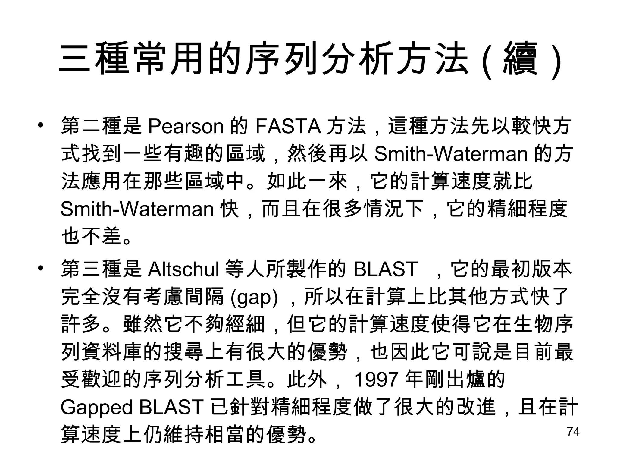

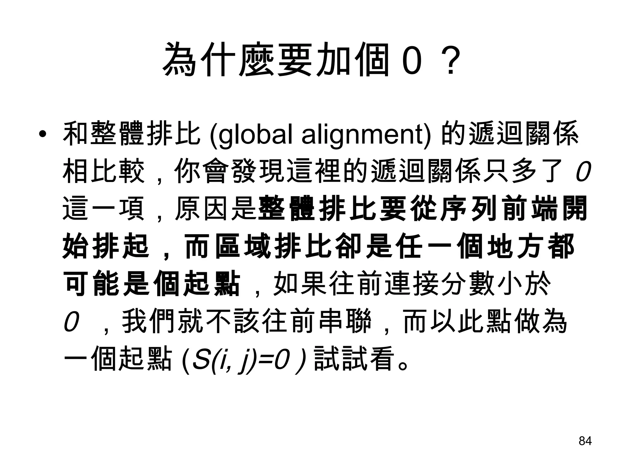
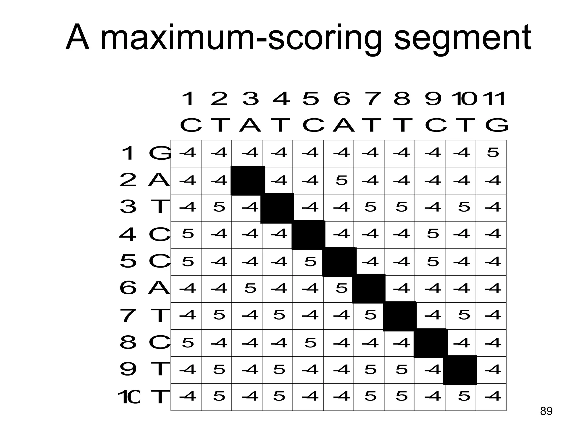
![多個最佳區域排比 有些人感興趣的是找出 k 個最好的區域排比或是分數至少有設定值那麼高的所有區域排比,這樣的計算在你熟悉動態規畫技巧後應不至於難倒你的。 上述的方式也就是一般俗稱的 Smith-Waterman 方法 ( 實際上,整體排比問題是由 Needleman 及 Wunsch[15] 所提出;而區域排比問題則是由 Smith 及 Waterman[21] 所提出 ) ,它基本上需要與兩序列長度乘積成常數正比的時間與空間。 在序列很長時,這種計算時間及空間都是很難令人接受的!](https://image.slidesharecdn.com/random-090723045308-phpapp02/75/2009-CSBB-LAB-85-2048.jpg)


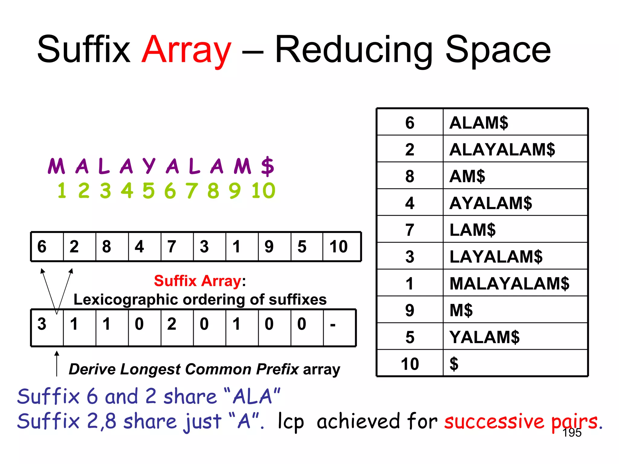
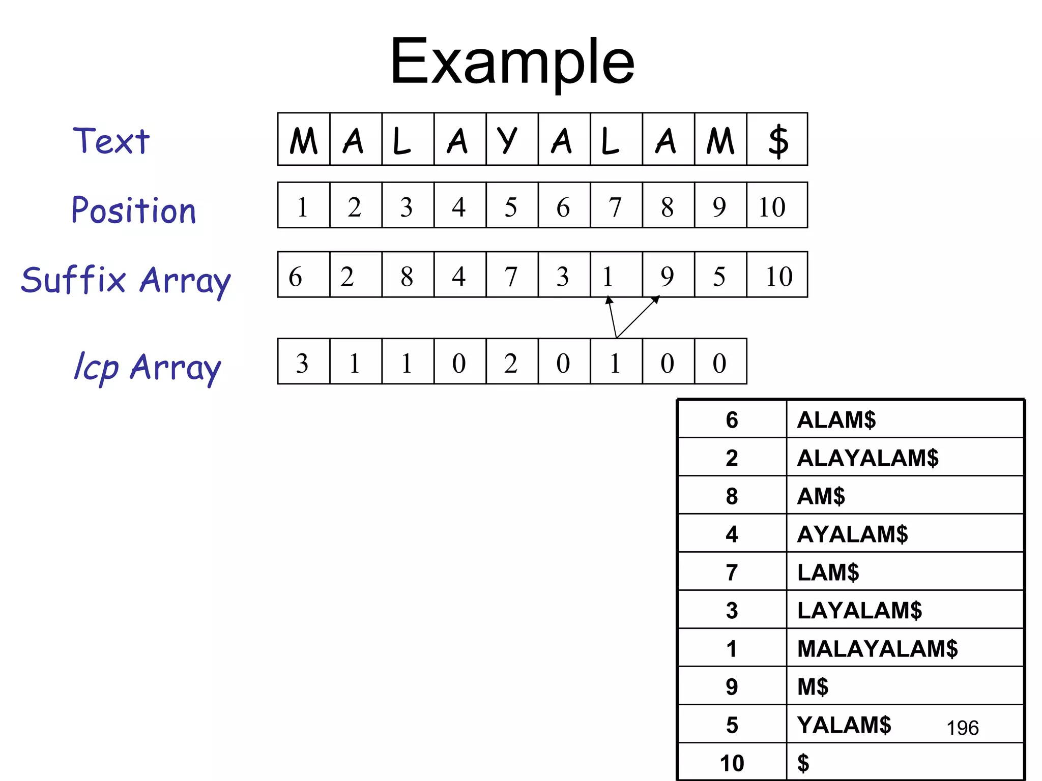
![Pattern Search in Suffix Array All suffixes that share a common prefix appear in consecutive positions in the array. Pattern P can be located in the string using a binary search on the suffix array. Naïve Run-time = O (|P| log n). Improved to O (|P| + log n) [Manber&Myers93], and to O(|P|) [Abouelhoda et al. 02].](https://image.slidesharecdn.com/random-090723045308-phpapp02/75/2009-CSBB-LAB-197-2048.jpg)
![Known (amazing) Results Suffix tree can be constructed in O ( n ) time and O ( n | ∑ |) space [Weiner73, McCreight76, Ukkonen92]. Suffix arrays can be constructed without using suffix trees in O ( n ) time [Pang&Aluru03].](https://image.slidesharecdn.com/random-090723045308-phpapp02/75/2009-CSBB-LAB-198-2048.jpg)
![More Applications Suffix-prefix overlaps in fragment assembly Maximal and tandem repeats Shortest unique substrings Maximal unique matches [MUMmer] Approximate matching Phylogenies based on complete genomes](https://image.slidesharecdn.com/random-090723045308-phpapp02/75/2009-CSBB-LAB-199-2048.jpg)
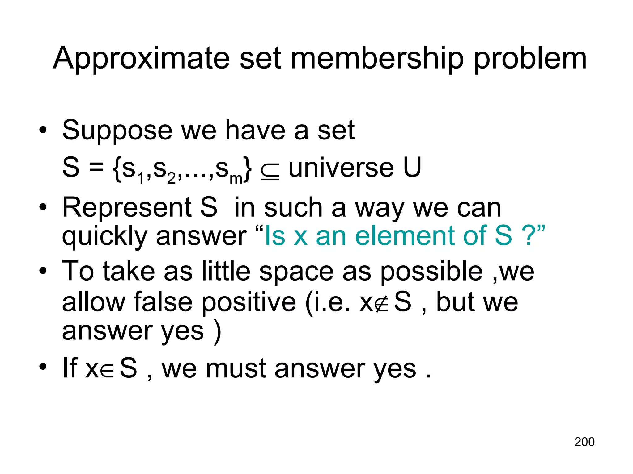
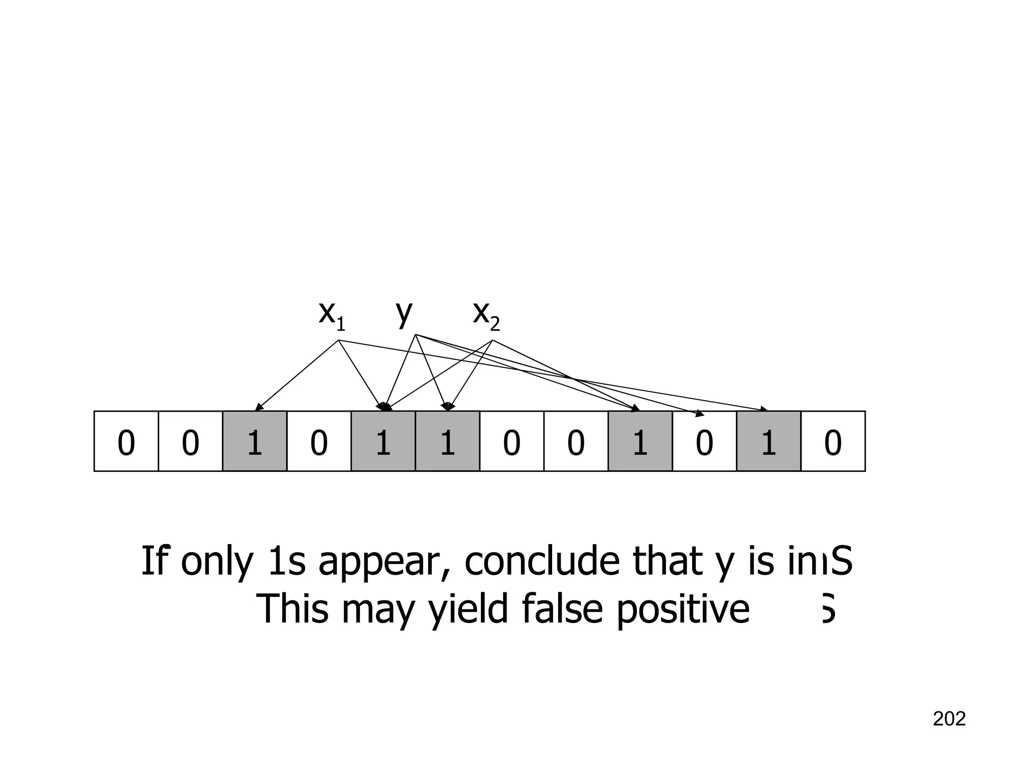
![Bloom filters Consist of an arrays A[n] of n bits (space) , and k independent random hash functions h 1 ,…,h k : U --> {0,1,..,n-1} 1. Initially set the array to 0 2. s S, A[h i (s)] = 1 for 1 i k (an entry can be set to 1 multiple times, only the first times has an effect ) 3. To check if x S , we check whether all location A[h i (x)] for 1 i k are set to 1 If not, clearly x S. If all A[h i (x)] are set to 1 ,we assume x S](https://image.slidesharecdn.com/random-090723045308-phpapp02/75/2009-CSBB-LAB-201-2048.jpg)

![Orthogonal Range Searching in 1D S: Set of points on real line. Q= Query Interval [a,b] a b Which query points lie inside the interval [a,b]?](https://image.slidesharecdn.com/random-090723045308-phpapp02/75/2009-CSBB-LAB-214-2048.jpg)
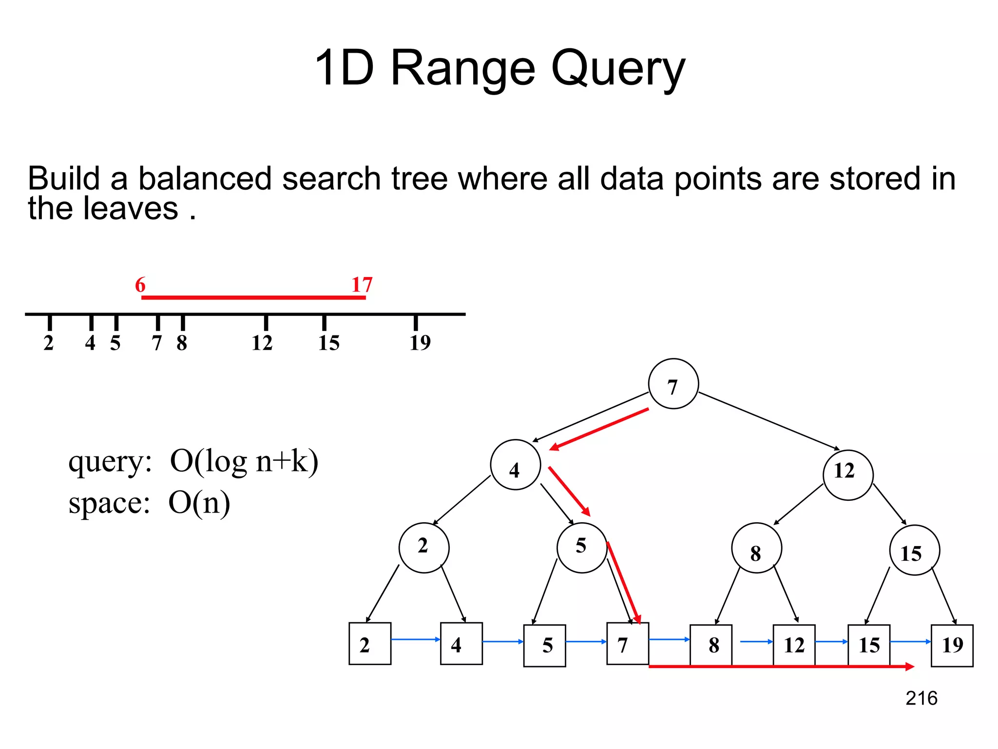
![Querying Strategy Given interval [a,b], search for a and b Find where the paths split, look at subtrees inbetween Paths split a b Problem: linking leaves do not extends to higher dimensions. Idea: if parents knew all descendants, wouldn’t need to link leaves.](https://image.slidesharecdn.com/random-090723045308-phpapp02/75/2009-CSBB-LAB-217-2048.jpg)
![1D Range Counting S = Set of points on real line Q= Query Interval [a,b] Count points in [a,b] Solution: At each node, store count of number of points in the subtree rooted at the node. Query: Similar to reporting but add up counts instead of reporting points. Query Time: O(log n)](https://image.slidesharecdn.com/random-090723045308-phpapp02/75/2009-CSBB-LAB-219-2048.jpg)
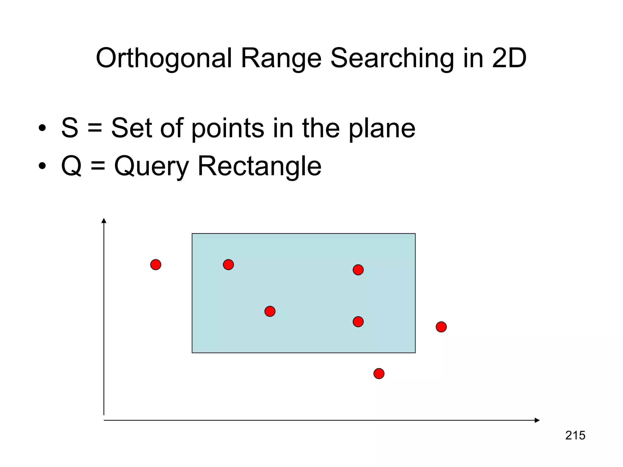
![2D Range queries How do you efficiently find points that are inside of a rectangle? Orthogonal range query ([ x 1 , x 2 ], [ y 1 ,y 2 ]): find all points ( x, y ) such that x 1 <x<x 2 and y 1 <y<y 2 x y x 1 x 2 y 1 y 2](https://image.slidesharecdn.com/random-090723045308-phpapp02/75/2009-CSBB-LAB-220-2048.jpg)
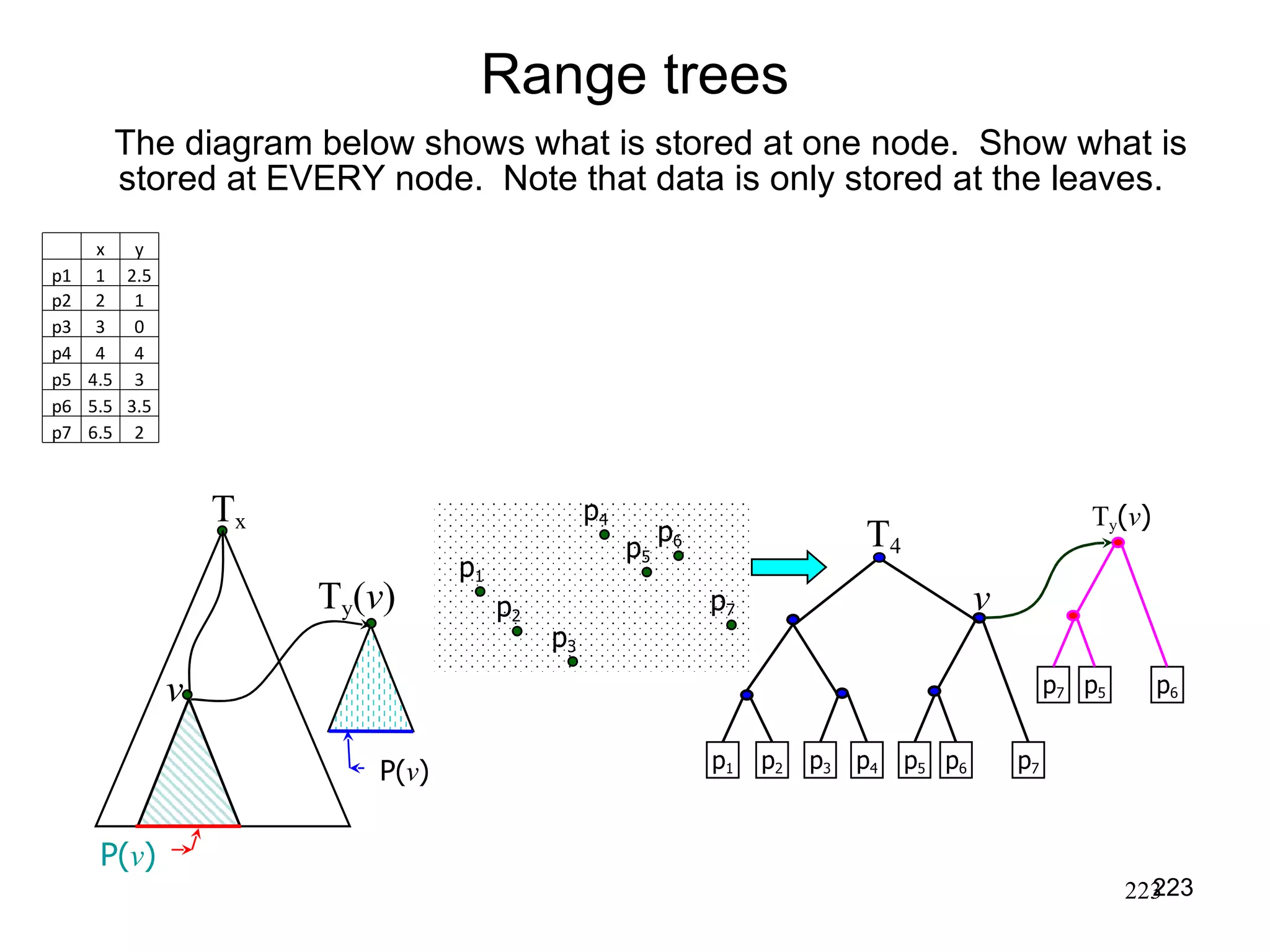
![Range trees The query time : Querying a 1D-tree requires O(log n+k) time. How many 1D trees (associated structures) do we need to query? At most 2 height of T = 2 log n Each 1D query requires O(log n+k’) time. Query time = O(log 2 n + k) Answer to query = Union of answers to subqueries: k = ∑k’ . Query: [x,x’] x x’](https://image.slidesharecdn.com/random-090723045308-phpapp02/75/2009-CSBB-LAB-224-2048.jpg)