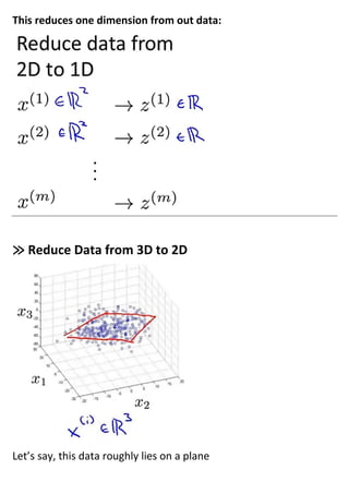
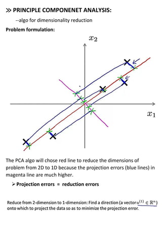
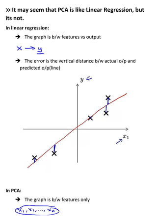
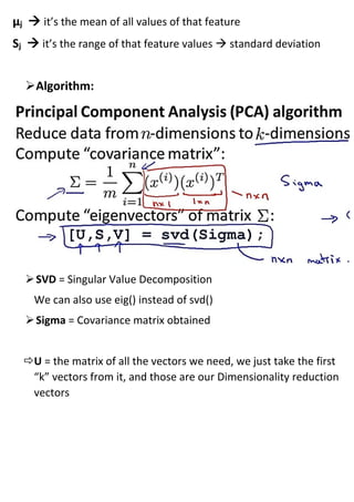
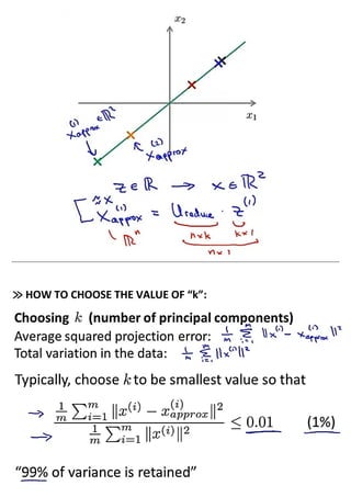
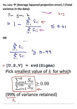
14. Dimensionality Reduction –
Unsupervised Learning Problem
It will allow us data compression and speeding up the
algorithm.
Example:
The points don’t lie on the straight line due to rounding off.
≫ Reduce Data from 2D to 1D
➢Since the two features are proportional (not exactly, just
approximately):
We try to project each data point on a line(green)
We represent this line as a new feature → z :
This reduces one dimension from out data:
≫ Reduce Data from 3D to 2D
Let’s say, this data roughly lies on a plane
So, we project the data on that plane:
Hence, we have reduced the data from 3D to 2D
Where:
Dimensionality reduction: Data Visualization:
Suppose we have a 50D feature vector
We have to find out two new features that can summarise these
50 features… then we can easily plot the data in 2D
We can use the two most important features of deviation
≫ PRINCIPLE COMPONENET ANALYSIS:
--algo for dimensionality reduction
Problem formulation:
The PCA algo will chose red line to reduce the dimensions of
problem from 2D to 1D because the projection errors (blue lines) in
magenta line are much higher.
➢Projection errors = reduction errors
More generally:
≫ It may seem that PCA is like Linear Regression, but
its not.
In linear regression:
➔ The graph is b/w features vs output
➔ The error is the vertical distance b/w actual o/p and
predicted o/p(line)
In PCA:
➔ The graph is b/w features only
➔ The error is projection of data on the PCA line.
≫ PRINCIPAL COMPOENT ANALYSIS – ALGOORITHM:
➢First we do the data pre-processing:
µj → it’s the mean of all values of that feature
Sj → it’s the range of that feature values → standard deviation
➢Algorithm:
➢SVD = Singular Value Decomposition
We can also use eig() instead of svd()
➢Sigma = Covariance matrix obtained
U = the matrix of all the vectors we need, we just take the first
“k” vectors from it, and those are our Dimensionality reduction
vectors
Now, to find the “z” feature vector:
Here, X → can be training data vector, cross validation, test data..
➔ It can also be a particular example: X( i )
≫ RECONSTRUCTION OF DATA FROM COMPRESSED
REPRESENTATION:
We have:
To approximate the original data:
≫ HOW TO CHOOSE THE VALUE OF “k”:
Algorithm:
We try diff values of k from 1 until we get the ratio ≤0.01 . But this
is not an efficient way: So, svd() saves us:
S→ n x n diagonal matrix
The ratio → (Average Squared projection error) / (Total
variance in the data):
OR
≫ Speedup Advice:
≫ Overfitting Advice:
≫ Misuse of PCA:
But instead:

14 dimentionality reduction

  • 1.
    14. Dimensionality Reduction– Unsupervised Learning Problem It will allow us data compression and speeding up the algorithm. Example: The points don’t lie on the straight line due to rounding off.
  • 2.
    ≫ Reduce Datafrom 2D to 1D ➢Since the two features are proportional (not exactly, just approximately): We try to project each data point on a line(green) We represent this line as a new feature → z :
  • 3.
    This reduces onedimension from out data: ≫ Reduce Data from 3D to 2D Let’s say, this data roughly lies on a plane
  • 4.
    So, we projectthe data on that plane: Hence, we have reduced the data from 3D to 2D Where:
  • 5.
    Dimensionality reduction: DataVisualization: Suppose we have a 50D feature vector We have to find out two new features that can summarise these 50 features… then we can easily plot the data in 2D We can use the two most important features of deviation
  • 6.
    ≫ PRINCIPLE COMPONENETANALYSIS: --algo for dimensionality reduction Problem formulation: The PCA algo will chose red line to reduce the dimensions of problem from 2D to 1D because the projection errors (blue lines) in magenta line are much higher. ➢Projection errors = reduction errors
  • 7.
  • 8.
    ≫ It mayseem that PCA is like Linear Regression, but its not. In linear regression: ➔ The graph is b/w features vs output ➔ The error is the vertical distance b/w actual o/p and predicted o/p(line) In PCA: ➔ The graph is b/w features only
  • 9.
    ➔ The erroris projection of data on the PCA line. ≫ PRINCIPAL COMPOENT ANALYSIS – ALGOORITHM: ➢First we do the data pre-processing:
  • 10.
    µj → it’sthe mean of all values of that feature Sj → it’s the range of that feature values → standard deviation ➢Algorithm: ➢SVD = Singular Value Decomposition We can also use eig() instead of svd() ➢Sigma = Covariance matrix obtained U = the matrix of all the vectors we need, we just take the first “k” vectors from it, and those are our Dimensionality reduction vectors
  • 11.
    Now, to findthe “z” feature vector: Here, X → can be training data vector, cross validation, test data.. ➔ It can also be a particular example: X( i )
  • 12.
    ≫ RECONSTRUCTION OFDATA FROM COMPRESSED REPRESENTATION: We have: To approximate the original data:
  • 13.
    ≫ HOW TOCHOOSE THE VALUE OF “k”:
  • 14.
    Algorithm: We try diffvalues of k from 1 until we get the ratio ≤0.01 . But this is not an efficient way: So, svd() saves us: S→ n x n diagonal matrix
  • 15.
    The ratio →(Average Squared projection error) / (Total variance in the data): OR
  • 16.
  • 17.
    ≫ Overfitting Advice: ≫Misuse of PCA: But instead: