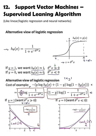
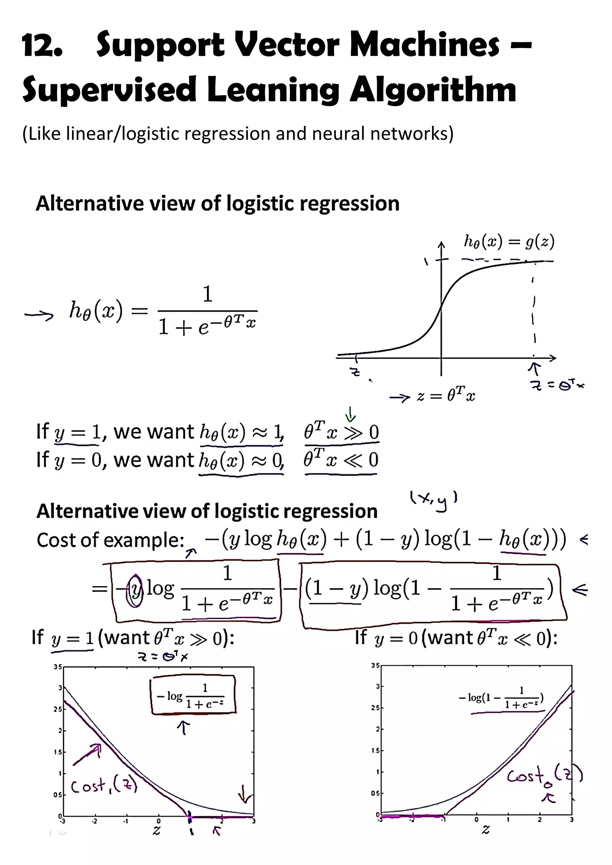
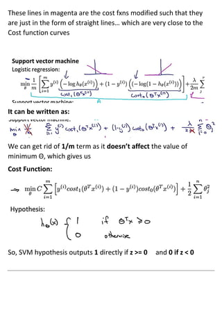
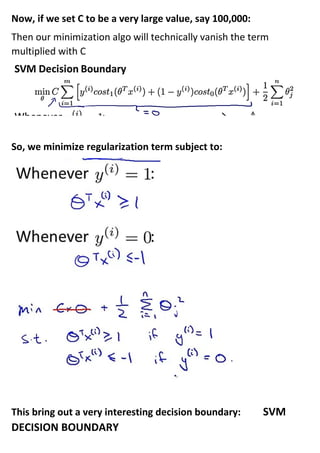
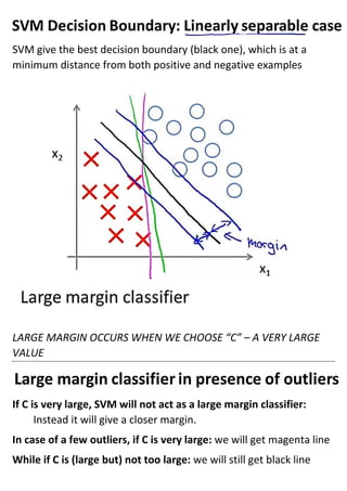
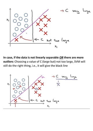
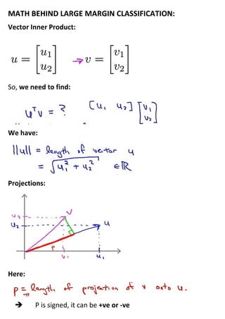
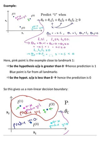
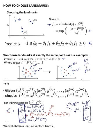
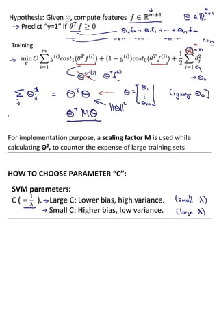
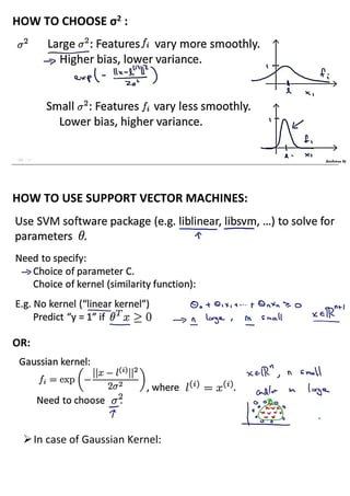
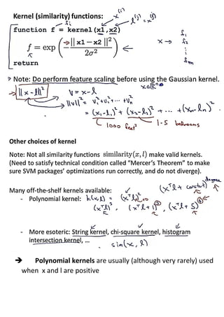
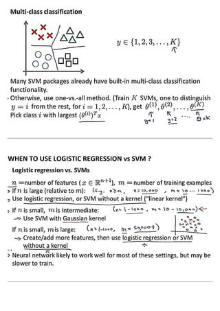
This document provides an overview of support vector machines (SVMs), a supervised machine learning algorithm. SVMs find a decision boundary that maximizes the margin between positive and negative examples. They do this by minimizing a cost function subject to constraints. Choosing a large value for the parameter C results in a large margin classifier, while a value that is large but not too large can still perform well even with outliers in the data. Kernels allow SVMs to find nonlinear decision boundaries by mapping data into higher dimensional feature spaces. The parameters C and sigma need to be chosen appropriately for good performance.

1. 12. Support Vector Machines –
Supervised Leaning Algorithm
(Like linear/logistic regression and neural networks)

2. These lines in magenta are the cost fxns modified such that they
are just in the form of straight lines… which are very close to the
Cost function curves
It can be written as:
We can get rid of 1/m term as it doesn’t affect the value of
minimum Θ, which gives us
Cost Function:
So, SVM hypothesis outputs 1 directly if z >= 0 and 0 if z < 0

3. Note:
In cost function, we use λ as the parameter to minimize the values
of Θ, but it can also be written as C.A + B… this just makes the same
effect if C=1/λ …
We use an acceptably large value of λ .. so we can use an
equivalrent small value of C to make the same effect and obtain the
same Θ
LARGE MARGIN INTUITION:
Here we want ΘT
x to be >=1 for positive examples as safety
margins
Similar for negative examples

4. Now, if we set C to be a very large value, say 100,000:
Then our minimization algo will technically vanish the term
multiplied with C
So, we minimize regularization term subject to:
This bring out a very interesting decision boundary: SVM
DECISION BOUNDARY

5. SVM give the best decision boundary (black one), which is at a
minimum distance from both positive and negative examples
LARGE MARGIN OCCURS WHEN WE CHOOSE “C” – A VERY LARGE
VALUE
If C is very large, SVM will not act as a large margin classifier:
Instead it will give a closer margin.
In case of a few outliers, if C is very large: we will get magenta line
While if C is (large but) not too large: we will still get black line

6. In case, if the data is not linearly separable OR there are more
outliers: Choosing a value of C (large but) not too large, SVM will
still do the right thing, i.e., it will give the black line

7. MATH BEHIND LARGE MARGIN CLASSIFICATION:
Vector Inner Product:
So, we need to find:
We have:
Projections:
Here:
➔ P is signed, it can be +ve or -ve

8. So, we get:
Matrix representation:
uTv =
Since p is signed:
If p < 0:

9. Optimization objective of SVM: Math behind it:
Why SVM gives large margin classification?
For simplification we take Θ0 = 0 and n = 2:
Θ0 = 0 → so that Θ vector passes through origin.
N=2 → only two features in the data
So, to find ΘT
x:
Therefore:

10. This gives us:
Let’s consider the case of small margin decision boundary: it’s not
a very good choice though:
➢Θ vector will be perpendicular to decision boundary as we can
recall that decision boundary does not depend on parameters
or hypothesis: it only depends on features.

11. Now lets plot the examples on this decision boundary:
This means that, since p( 1 )
and p( 2 )
are small, for p( 1 )||Θ|| to
be greater than 1:
||Θ|| will have to be large.
But this contradicts our cost minimization efforts, So, this decision
boundary is not the chosen
Now suppose a large margin decision boundary is chosen:

12. Since p( 1 )
is larger, Θ can be smaller, which supports are norm of
minimizing Θ in cost function’s regularization part.
➢The values of margin is equal to the values of p for given
example
KERNELS:
To write complex non-linear classifiers
Usually what we do is:
This is how we define features for our hypothesis.
But:

13. Landmarks are some vectors on the feature vs feature graph
Similarity can also be written as:
➢||x – l( 1 )
|| is the component wise difference bw vector x
and vector l.

14. What are kernels:
Lets try diff values of σ :

15. If we decr σ:
More values of x will be close to 0.
If we incr σ :
More values of x will be higher than 0.

16. Example:
Here, pink point is the example close to landmark 1:
So the hypothesis o/p is greater than 0 →hence prediction is 1
Blue point is far from all landmarks
So the hypot. o/p is less than 0 → hence the prediction is 0
So this gives us a non-linear decision boundary:

17. HOW TO CHOOSE LANDMARKS:
We choose landmarks at exactly the same points as our examples:
→→
We will obtain a feature vector f from x.

18. For implementation purpose, a scaling factor M is used while
calculating Θ2
, to counter the expense of large training sets
HOW TO CHOOSE PARAMETER “C”:

19. HOW TO CHOOSE σ2 :
HOW TO USE SUPPORT VECTOR MACHINES:
OR:
➢In case of Gaussian Kernel:

20. ➔ Polynomial kernels are usually (although very rarely) used
when x and l are positive

21. WHEN TO USE LOGISTIC REGRESSION vs SVM ?