Excel for
Analytics
EXCEL- Reading Data
Reading Data into Excel using various format
⮚ Regular Excel Format(.xlsx,.xls)
⮚ Text Format(.txt)
EXCEL- Predefined functions
⮚ ROUND(): returns a number rounded to a specified number of
digits
⮚ SQRT(): returns square root of a number
⮚ MIN()/MAX(): returns the smallest/largest numeric value in a range
of values
⮚ SUM(): returns the sum of a range of values
⮚ AVERAGE(): returns the average or mean value of a range of
values
⮚ MEDIAN(): returns the median value of a range of values
⮚ RANK(): used to find the rank of a number in a list of numbers
⮚ LEFT()/RIGHT(): extracts a given number of characters from the
left side/right side of a supplied text string
⮚ LEN(): used to find the length of a text string
EXCEL- Advanced Functions
DateTime
⮚ DATE(): creates a valid date from individual
year, month, and day components
⮚ EOMONTH(): Returns the serial number for the
last day of the month that is the indicated
number of months before or after start date
⮚ NETWORKDAYS(): calculates the number of
workdays between two dates in Excel
⮚ WEEKDAY(): returns a number between 1-7
representing the day of week.
DATE() WEEKDAY()
EOMONTH()
NETWORKDAYS(
)
Database Functions
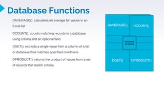
⮚ DAVERAGE(): calculates an average for values in an
Excel list
⮚ DCOUNT(): counts matching records in a database
using criteria and an optional field
⮚ DGET(): extracts a single value from a column of a list
or database that matches specified conditions
⮚ DPRODUCT(): returns the product of values from a set
of records that match criteria
DAVERAGE() DCOUNT()
DGET() DPRODUCT()
Database
functions
⮚ FIND(): returns the location of a substring in a string
⮚ REPLACE(): replaces characters specified by location in a
given text string with another text string
⮚ SUBSTITUTE(): replaces text in a given string by matching
⮚ MID(): extracts a given number of characters from the middle
of a supplied text string
⮚ SEARCH(): used to find the position of a character inside a text
string
⮚ CONCAT(): used to join two or more text strings into one string
Text Functions
EXCEL- Advanced Functions
FIND() REPLACE()
SUBSTITUTE() MID()
SEARCH() CONCATENATE()
EXCEL- Advanced Functions
Mathematical Functions
⮚ PRODUCT(): returns the product of numbers provided as arguments
=PRODUCT (number1, [number2], ...)
⮚ MOD(): returns the remainder of two numbers after division
=MOD (number, divisor)
⮚ SQRT(): returns the square root of a positive number
=SQRT (number)
⮚ FACT(): returns the factorial of a given number
⮚ ROUNDUP()/ROUNDDOWN(): round the number
upward/downward to the specified number of digits
=ROUNDUP (number, num_digits)
⮚ SUMIFS(): adds all of its arguments that meet multiple criteria
=SUMIFS (sum_range, range1, criteria1, [range2], [criteria2], ...)
PRODUCT() MOD()
SQRT() FACT()
ROUNDUP() ROUNDDOWN()
SUMIFS()
EXCEL- Advanced Functions
HLOOKUP and VLOOKUP are functions in Microsoft Excel
that allow you to use a section of your spreadsheet as a
lookup table.
When the VLOOKUP function is called, Excel searches for a
lookup value in the leftmost column of a section of your
spreadsheet called the table array. The function returns
another value in the same row, defined by the column index
number.
HLOOKUP is similar to VLOOKUP, but searches a row instead
of a column, and the result is offset by a row index number.
The V in VLOOKUP stands for vertical search (in a single
column), while the H in HLOOKUP stands for horizontal
search (within a single row).
Lookup Functions
EXCEL- Advanced Functions
⮚ HLOOKUP(): makes Excel search for a certain value in a row (the so called
'table array’) =HLOOKUP("Axles", A1:C4, 2, TRUE)
Looks up "Axles" in row 1, and returns the value from row 2 that's in the same
column (column A) Result: 4
⮚ VLOOKUP(): =VLOOKUP(What you want to look up, where you want to look
for it, the column number in the range containing the value to return,
Approximate or Exact match – indicated as 1/TRUE, or 0/FALSE)
⮚ MATCH(): used to locate the position of a lookup value in a row, column, or
table
=MATCH (lookup_value, lookup_array, [match_type])
⮚ INDEX(): returns the value at a given location in a range or array
=INDEX (array, row_num, [col_num], [area_num])
Lookup Functions
1
• HLOOKUP()
2
• VLOOKUP()
3
• MATCH()
4
• INDEX()
EXCEL- Advanced Functions
Logical and Error Functions
⮚ AND: used to require more than one condition at the same time
⮚ OR: a logical function to test multiple conditions at the same time
⮚ NOT: The function helps check if one value is not equal to another
⮚ ISERROR: returns TRUE for any error type excel generates, including #N/A,
#VALUE!, #REF!, #DIV/0!, #NUM!, #NAME?, or #NULL
⮚ ISNUMBER: The function checks if a cell in Excel contains a number or not. It will
return TRUE if the value is a number and if not, a FALSE value
⮚ ISBLANK: returns TRUE when a cell contains is empty, and FALSE when a cell is
not empty
⮚ IF: Test for a specific condition. =IF (logical_test, [value_if_true], [value_if_false])
⮚ IFERROR: returns a custom result when a formula generates an error, and a
standard result when no error is detected
AND
OR
ISERROR
ISNUMBER
ISBLANK
IF
IFERROR
EXCEL- Advanced Functions
⮚ COUNT(): to get the number of entries in a number
field that is in a range or array of numbers
⮚ COUNTA(): returns the count of cells that contain
numbers, text, logical values, error values, and
empty text (""). COUNTA does not count empty cells
⮚ COUNTBLANK(): returns a count of empty cells in a
range
⮚ COUNTIFS(): counts the number of cells in a range
that match one supplied criteria
Statistical Functions
COUNT() COUNTA()
COUNTBLANK() COUNTIFS()
⮚ MEAN: Get the average of a group of numbers.
Syntax = AVERAGE (number1, [number2], ...)
⮚ MEDIAN(): Get the median of a group of
numbers. Syntax = AVERAGE (number1,
[number2], ...)
⮚ MODE(): returns the most frequently occurring
number in a numeric data set.
⮚ CORREL: used to find out the correlation
coefficient between two variables.
CORREL(array1, array2)
⮚ STDEV: returns the statistical rank of a given
value within a supplied array of values
Statistical
Functions
MEAN
MEDIAN()
MODE()
CORREL()
STDEV
Formatting
Excel formatting is an optional
step following data preparation,
or all of the data cleansing,
enriching, structuring, and
standardizing that is required in
order to prepare data for analysis.
For example, adding $ to cells
that contain values pertaining to
prices or configuring cells that
represent dates to a standard
display of xx/xx/xxxx
Components of
Format Cells
⮚ Number
⮚ Alignment
⮚ Font
⮚ Border
⮚ Fill
⮚ Protection
Formatting
Data Formatting
Custom Formatting
Formatting
Understand how to use Custom Formatting to format number and date values
Conditional Formatting
Formatting
Illustrate the use of conditional formatting in Excel
⮚ Conditional formatting helps us visualize data and make
worksheets easier to understand
⮚ It quickly highlights important information in a spreadsheet by
using colors, icons, and data bars
⮚ It changes the appearance of one or more cells when cell values
meet certain conditions
Formatting
Conditional Formatting
Charts in Excel
You’ll learn these things:
⮚ Inserting a Chart
⮚ Adjusting a Chart
⮚ Improving a Chart
⮚ Add series to a chart
⮚ Create Combination Charts
MS Excel
Excel Online
Google Sheets
All are in a way similar in nature
Charts in Excel
Statistical Analysis using Excel
Let’s see how do we perform various statistical tests in Excel
First of all, is it possible to perform the same Statistical tests
in Excel that we usually perform in Python
The answer is YES!!
Data Analysis using Excel
Analysing Data with Pivot Tables
Doing a proper analysis of the available data helps companies make critical business decisions. But sometimes
it’s difficult to understand where to start, especially when the data is huge
Analysing Data with Pivot Tables
One can design a PivotTable by simply, dragging and dropping relevant information into the appropriate
boxes. This tool quickly pivots or reorganizes data allowing us to answer different questions and even
experiment with the data to discover new trends and patterns
How it works…
Analysing Data with Pivot Tables
A PivotTable helps to extract the important
information from a large, detailed dataset.
Sometimes, the focus is required on just a
certain section of our data. Filters help us
narrow down the data in the PivotTable,
extracting the required information
Filters
Analysing Data with Pivot Tables
Another important tool of Excel, Slicers, makes
filtering data in PivotTables even easier. Slicers
contain a set of buttons which make filtering data in
PivotTables easier and quicker. We do not have to
open the drop-down lists to find the items we want to
filter. We can create slicers for any field and can filter
a Pivot Table by selecting the type of data we want.
Slicers
Analysing Data with Pivot Tables
It is often useful to group the fields in a
PivotTable by the header values.
Grouping data in a PivotTable allows
us to group the data for any field
added as a row or a column. Excel
can do this automatically for numeric
values (including dates and time).
Grouping
Analysing Data with Pivot Tables
Sometimes, there is a need to change the way the values are displayed in the PivotTable.
The value can be displayed in terms of a percentage instead of a total or an average of the values instead
of summing them
Custom Calculation
Analysing Data with Pivot Tables
Once we have created a PivotTable, we can add calculated fields
and calculated items in it
⮚ Calculated fields help us enhance the results by allowing us to
write our own formulas. This functionality helps to create a new
field in the table that performs the calculations based on other
pivot fields. Let us understand how to use these fields with the
help of an example..
⮚ We can also add one or more calculated items in a PivotTable
field apart from the existing items. Calculated items are used
to perform calculations between items within the fields
Calculated Field and Calculated Item
Analysing Data with Pivot Tables
Calculated Field and Calculated Item
Dashboarding
⮚ Create and format different types of charts such as Thermometer and Pareto Charts
⮚ Importance of interactive charts
⮚ Form Controls such as Combo box, Check box, and Radio buttons
An appropriately designed dashboard can:
⮚ Quicken decision-making processes
⮚ Provide better coordination for your
organization’s efforts
⮚ Record the performance outcome
Dashboarding
⮚ Using dashboards, the data visualization tool of Excel, it is easy to create the detailed
analysis reports.
⮚ These dashboard reports will provide insights and alert us in case of negative trends or
projections for Profit/Sales in specific regions which can then be used to develop
future strategy.
⮚ Dashboards are highly effective in validating the effectiveness of the matrices
captured over time and bringing out the leading trends.
⮚ Dashboards help consolidate and organize these metrics through a summary.
Dashboarding
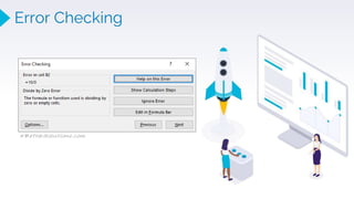
Error Checking
Show Formulas
Text to Column
Data Validation
Sort And Filter
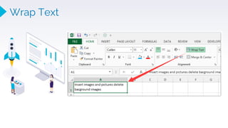
Wrap Text
Merge Cell & Insert Comments
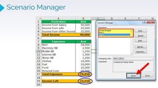
What-if Tools
What-If Analysis is the process of changing the values in cells to see
how those changes will affect the outcome of formulas on the
worksheet. Three kinds of What-If Analysis tools come with Excel:
Scenarios, Goal Seek, and Data Tables. Scenarios and Data tables
take sets of input values and determine possible results.
Scenario Manager
Data Table
VBA & Macros
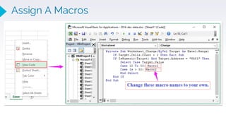
Assign A Macros
Record A Macros

1.2 Zep Excel.pptx

  • 1.
  • 2.
    EXCEL- Reading Data ReadingData into Excel using various format ⮚ Regular Excel Format(.xlsx,.xls) ⮚ Text Format(.txt)
  • 3.
    EXCEL- Predefined functions ⮚ROUND(): returns a number rounded to a specified number of digits ⮚ SQRT(): returns square root of a number ⮚ MIN()/MAX(): returns the smallest/largest numeric value in a range of values ⮚ SUM(): returns the sum of a range of values ⮚ AVERAGE(): returns the average or mean value of a range of values ⮚ MEDIAN(): returns the median value of a range of values ⮚ RANK(): used to find the rank of a number in a list of numbers ⮚ LEFT()/RIGHT(): extracts a given number of characters from the left side/right side of a supplied text string ⮚ LEN(): used to find the length of a text string
  • 4.
    EXCEL- Advanced Functions DateTime ⮚DATE(): creates a valid date from individual year, month, and day components ⮚ EOMONTH(): Returns the serial number for the last day of the month that is the indicated number of months before or after start date ⮚ NETWORKDAYS(): calculates the number of workdays between two dates in Excel ⮚ WEEKDAY(): returns a number between 1-7 representing the day of week. DATE() WEEKDAY() EOMONTH() NETWORKDAYS( )
  • 5.
    Database Functions ⮚ DAVERAGE():calculates an average for values in an Excel list ⮚ DCOUNT(): counts matching records in a database using criteria and an optional field ⮚ DGET(): extracts a single value from a column of a list or database that matches specified conditions ⮚ DPRODUCT(): returns the product of values from a set of records that match criteria DAVERAGE() DCOUNT() DGET() DPRODUCT() Database functions
  • 6.
    ⮚ FIND(): returnsthe location of a substring in a string ⮚ REPLACE(): replaces characters specified by location in a given text string with another text string ⮚ SUBSTITUTE(): replaces text in a given string by matching ⮚ MID(): extracts a given number of characters from the middle of a supplied text string ⮚ SEARCH(): used to find the position of a character inside a text string ⮚ CONCAT(): used to join two or more text strings into one string Text Functions EXCEL- Advanced Functions FIND() REPLACE() SUBSTITUTE() MID() SEARCH() CONCATENATE()
  • 7.
    EXCEL- Advanced Functions MathematicalFunctions ⮚ PRODUCT(): returns the product of numbers provided as arguments =PRODUCT (number1, [number2], ...) ⮚ MOD(): returns the remainder of two numbers after division =MOD (number, divisor) ⮚ SQRT(): returns the square root of a positive number =SQRT (number) ⮚ FACT(): returns the factorial of a given number ⮚ ROUNDUP()/ROUNDDOWN(): round the number upward/downward to the specified number of digits =ROUNDUP (number, num_digits) ⮚ SUMIFS(): adds all of its arguments that meet multiple criteria =SUMIFS (sum_range, range1, criteria1, [range2], [criteria2], ...) PRODUCT() MOD() SQRT() FACT() ROUNDUP() ROUNDDOWN() SUMIFS()
  • 8.
    EXCEL- Advanced Functions HLOOKUPand VLOOKUP are functions in Microsoft Excel that allow you to use a section of your spreadsheet as a lookup table. When the VLOOKUP function is called, Excel searches for a lookup value in the leftmost column of a section of your spreadsheet called the table array. The function returns another value in the same row, defined by the column index number. HLOOKUP is similar to VLOOKUP, but searches a row instead of a column, and the result is offset by a row index number. The V in VLOOKUP stands for vertical search (in a single column), while the H in HLOOKUP stands for horizontal search (within a single row). Lookup Functions
  • 9.
    EXCEL- Advanced Functions ⮚HLOOKUP(): makes Excel search for a certain value in a row (the so called 'table array’) =HLOOKUP("Axles", A1:C4, 2, TRUE) Looks up "Axles" in row 1, and returns the value from row 2 that's in the same column (column A) Result: 4 ⮚ VLOOKUP(): =VLOOKUP(What you want to look up, where you want to look for it, the column number in the range containing the value to return, Approximate or Exact match – indicated as 1/TRUE, or 0/FALSE) ⮚ MATCH(): used to locate the position of a lookup value in a row, column, or table =MATCH (lookup_value, lookup_array, [match_type]) ⮚ INDEX(): returns the value at a given location in a range or array =INDEX (array, row_num, [col_num], [area_num]) Lookup Functions 1 • HLOOKUP() 2 • VLOOKUP() 3 • MATCH() 4 • INDEX()
  • 10.
    EXCEL- Advanced Functions Logicaland Error Functions ⮚ AND: used to require more than one condition at the same time ⮚ OR: a logical function to test multiple conditions at the same time ⮚ NOT: The function helps check if one value is not equal to another ⮚ ISERROR: returns TRUE for any error type excel generates, including #N/A, #VALUE!, #REF!, #DIV/0!, #NUM!, #NAME?, or #NULL ⮚ ISNUMBER: The function checks if a cell in Excel contains a number or not. It will return TRUE if the value is a number and if not, a FALSE value ⮚ ISBLANK: returns TRUE when a cell contains is empty, and FALSE when a cell is not empty ⮚ IF: Test for a specific condition. =IF (logical_test, [value_if_true], [value_if_false]) ⮚ IFERROR: returns a custom result when a formula generates an error, and a standard result when no error is detected AND OR ISERROR ISNUMBER ISBLANK IF IFERROR
  • 11.
    EXCEL- Advanced Functions ⮚COUNT(): to get the number of entries in a number field that is in a range or array of numbers ⮚ COUNTA(): returns the count of cells that contain numbers, text, logical values, error values, and empty text (""). COUNTA does not count empty cells ⮚ COUNTBLANK(): returns a count of empty cells in a range ⮚ COUNTIFS(): counts the number of cells in a range that match one supplied criteria Statistical Functions COUNT() COUNTA() COUNTBLANK() COUNTIFS()
  • 12.
    ⮚ MEAN: Getthe average of a group of numbers. Syntax = AVERAGE (number1, [number2], ...) ⮚ MEDIAN(): Get the median of a group of numbers. Syntax = AVERAGE (number1, [number2], ...) ⮚ MODE(): returns the most frequently occurring number in a numeric data set. ⮚ CORREL: used to find out the correlation coefficient between two variables. CORREL(array1, array2) ⮚ STDEV: returns the statistical rank of a given value within a supplied array of values Statistical Functions MEAN MEDIAN() MODE() CORREL() STDEV
  • 13.
    Formatting Excel formatting isan optional step following data preparation, or all of the data cleansing, enriching, structuring, and standardizing that is required in order to prepare data for analysis. For example, adding $ to cells that contain values pertaining to prices or configuring cells that represent dates to a standard display of xx/xx/xxxx Components of Format Cells ⮚ Number ⮚ Alignment ⮚ Font ⮚ Border ⮚ Fill ⮚ Protection
  • 14.
  • 15.
    Custom Formatting Formatting Understand howto use Custom Formatting to format number and date values
  • 16.
    Conditional Formatting Formatting Illustrate theuse of conditional formatting in Excel ⮚ Conditional formatting helps us visualize data and make worksheets easier to understand ⮚ It quickly highlights important information in a spreadsheet by using colors, icons, and data bars ⮚ It changes the appearance of one or more cells when cell values meet certain conditions
  • 17.
  • 18.
    Charts in Excel You’lllearn these things: ⮚ Inserting a Chart ⮚ Adjusting a Chart ⮚ Improving a Chart ⮚ Add series to a chart ⮚ Create Combination Charts MS Excel Excel Online Google Sheets All are in a way similar in nature
  • 19.
  • 20.
    Statistical Analysis usingExcel Let’s see how do we perform various statistical tests in Excel First of all, is it possible to perform the same Statistical tests in Excel that we usually perform in Python The answer is YES!!
  • 21.
  • 22.
    Analysing Data withPivot Tables Doing a proper analysis of the available data helps companies make critical business decisions. But sometimes it’s difficult to understand where to start, especially when the data is huge
  • 23.
    Analysing Data withPivot Tables One can design a PivotTable by simply, dragging and dropping relevant information into the appropriate boxes. This tool quickly pivots or reorganizes data allowing us to answer different questions and even experiment with the data to discover new trends and patterns How it works…
  • 24.
    Analysing Data withPivot Tables A PivotTable helps to extract the important information from a large, detailed dataset. Sometimes, the focus is required on just a certain section of our data. Filters help us narrow down the data in the PivotTable, extracting the required information Filters
  • 25.
    Analysing Data withPivot Tables Another important tool of Excel, Slicers, makes filtering data in PivotTables even easier. Slicers contain a set of buttons which make filtering data in PivotTables easier and quicker. We do not have to open the drop-down lists to find the items we want to filter. We can create slicers for any field and can filter a Pivot Table by selecting the type of data we want. Slicers
  • 26.
    Analysing Data withPivot Tables It is often useful to group the fields in a PivotTable by the header values. Grouping data in a PivotTable allows us to group the data for any field added as a row or a column. Excel can do this automatically for numeric values (including dates and time). Grouping
  • 27.
    Analysing Data withPivot Tables Sometimes, there is a need to change the way the values are displayed in the PivotTable. The value can be displayed in terms of a percentage instead of a total or an average of the values instead of summing them Custom Calculation
  • 28.
    Analysing Data withPivot Tables Once we have created a PivotTable, we can add calculated fields and calculated items in it ⮚ Calculated fields help us enhance the results by allowing us to write our own formulas. This functionality helps to create a new field in the table that performs the calculations based on other pivot fields. Let us understand how to use these fields with the help of an example.. ⮚ We can also add one or more calculated items in a PivotTable field apart from the existing items. Calculated items are used to perform calculations between items within the fields Calculated Field and Calculated Item
  • 29.
    Analysing Data withPivot Tables Calculated Field and Calculated Item
  • 30.
    Dashboarding ⮚ Create andformat different types of charts such as Thermometer and Pareto Charts ⮚ Importance of interactive charts ⮚ Form Controls such as Combo box, Check box, and Radio buttons An appropriately designed dashboard can: ⮚ Quicken decision-making processes ⮚ Provide better coordination for your organization’s efforts ⮚ Record the performance outcome
  • 31.
    Dashboarding ⮚ Using dashboards,the data visualization tool of Excel, it is easy to create the detailed analysis reports. ⮚ These dashboard reports will provide insights and alert us in case of negative trends or projections for Profit/Sales in specific regions which can then be used to develop future strategy. ⮚ Dashboards are highly effective in validating the effectiveness of the matrices captured over time and bringing out the leading trends. ⮚ Dashboards help consolidate and organize these metrics through a summary.
  • 32.
  • 33.
  • 34.
  • 35.
  • 36.
  • 37.
  • 38.
  • 39.
    Merge Cell &Insert Comments
  • 40.
    What-if Tools What-If Analysisis the process of changing the values in cells to see how those changes will affect the outcome of formulas on the worksheet. Three kinds of What-If Analysis tools come with Excel: Scenarios, Goal Seek, and Data Tables. Scenarios and Data tables take sets of input values and determine possible results.
  • 41.
  • 42.
  • 43.
  • 44.
  • 45.