Download to read offline
![4. Redundancy Allocation
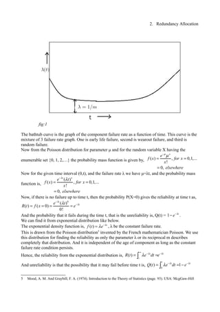
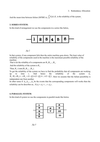
In this kind of system the entire machine works until the single component works. Hence the
maximum value of the reliabilities of the components is the minimum possible value of the
reliability of the machine.
1 2 n
s
s 1 2 n
That is let the reliablity of n components are R ,R ,...,R .
And the reliability of the system is R .
Then, R max{R ,R ,...,R }.≥
Now the reliability of the system we have to find the probability that at least one system will work
at that particular time. Which will be, 1 2 nP(A A ... A )U U U .
In another sense the machine will fail if all the components fail simultaneously. That probability is
1 2 nQ Q ... Q× × × . Hence the reliability of the system will be, s 1 2 nR =1-Q Q ... Q× × × .
5. PARALLEL SYSTEM VERSUS SERIES SYSTEM :
Now we will see that the parallel system is more reliable than series system.
We can show this by 2 ways,
1> By showing, 1 2 1 2 n(1 ) (1 ) ... (1 ) 1-Q Q ... QnQ Q Q− × − × × − ≤ × × ×
2> Or,
As, the events are independent then (2) becomes, 1 2 n 1 2 n(A ) (A )...P(A ) P(A A ... A )P P ≤ U U U .
For (1) we can prove like below.
(2) can be proved as,
1 2 1 2
1 2 1 2 1 2 1 2 1 2 1 2
1 2
1 2
, ( ) : (1- )(1- )...(1- ) 1- ...
(1) .
, (1- )(1- ) 1- - 1 -
1-
, (2) .
( )
(1- )(1- )
n nLet P n Q Q Q Q Q Q
Then P is true
Now Q Q Q Q Q Q Q Q Q Q Q Q
Q Q
So P is true
Let P m is true
Then Q Q
≤
= + ≤ − +
=
1 1 2 1
1 1 2 1 2 1
1 2 1
...(1- )(1- ) (1- ... )(1- )
[ sin ( )]
1- - ... ...
1 ...
( )
m m m m
m m m m
m m
Q Q Q Q Q Q
u g P m
Q Q Q Q Q Q Q Q
Q Q Q Q
Hence P m is tr
+ +
+ +
+
≤
≤ +
≤ −
( ) . (1), (2) .
( )
.
ue if P m is true Again P P are true
Hence by principle of mathematical induction P n is true for
all n N∈
1 2 1 2( ... ) ( ... )n nP A A A P A A A∩ ∩ ∩ ≤ U U U](https://image.slidesharecdn.com/1untitled1-140327090005-phpapp02/85/1-untitled-1-4-320.jpg)

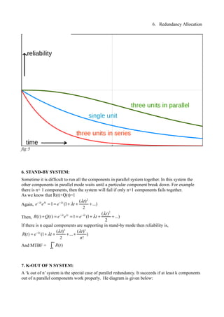
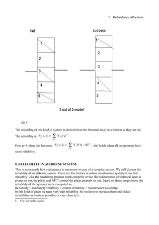
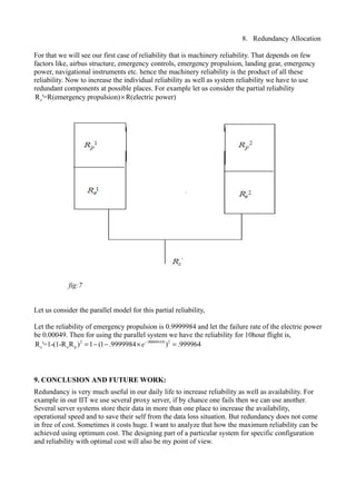

This document discusses redundancy allocation, which is a concept to increase system reliability by using components in parallel rather than series. It defines key reliability terms like MTBF and explains how parallel systems are more reliable than series systems. Specific redundancy concepts covered include standby redundancy, where extra components act as backups, and k-out-of-n systems, where the system succeeds if at least k out of n components work. The document also provides an example of applying redundancy to increase the reliability of an aircraft's emergency systems.