International Journal of Research in Advent Technology, Vol.7, No.1, January 2019
E-ISSN: 2321-9637
Available online at www.ijrat.org
273
Optimal N-Policy for Bernoulli feedback Mx
/G/1 Machining
System
Krishna Gopal Varshney, Dr.Rajvir Singh
(1) Departments of Mathematics,
Government Degree College,Kasganj (U.P.)
(Affiliated to Dr.B.R. Ambedkar University Agra)
(2) Basic Education Department, Mainpuri (U.P.)
E-mail : kgp123mayanath@gmail.com, rajshakya1582@gmail.com
Abstract- This study applies N-policy to an MX
/G/1 repairable machining system with Bernoulli feedback and general
setup time. The arrival rate of the failed units depends on the state of the system which may be in buildup, setup and busy
states. Supplementary variable technique is employed to obtain the probability generating function for the system queue
size distribution and the mean number of failed units in the system under steady state conditions. The Laplace-Stieltjes
transform of the waiting time is obtained which is further used to evaluate its mean value. The total operational cost of the
system is minimized in order to determine the optimal value of N.
Keywords: N-Policy, MX
/G/1 system, Batch arrival, Bernoulli feedback, Setup time, Supplementary variable technique,
Queue size, waiting time.
1. INTRODUCTION
Queueing theory has emerged as one of the foremost
areas of research because of its utility in simulating
many real life systems.we proposed an optimal control
N-policy for an M/Ek/1 system. We now shift our focus
to a batch failure queueing model with feedback. Many
congestion situations arising in data communication and
telecommunication systems can be modeled as feedback
queueing models where a unit receiving incomplete
service may repeatedly seek service till its service is
completed. In recent past, queueing systems with
Bernoulli feedback have been extensively investigated
by Disney et al. (1980), Simon (1984) and many others.
An M/G/1 queue with Bernoulli feedback was studied
by Rege (1993). Retrial queues with Bernoulli feedback
have been analysed by Krishna Kumar et al. (2002) and
recently by Atencia and Moreno (2004).
In many realistic situations, customers arrive in
batches. Burke (1975) and Chaudhary and Templeton
(1983) have contributed significantly to the study the
bulk arrival queues. Lee and Lee (1991) examined an
M/G/1 batch arrival queue with different server
vacations. Batch arrival queues have been thoroughly
investigated by Lee et al. (1995), Yue and Cao (1997),
Lee et al. (1998), Bacot and Dshalalow (2001) and
others. Chaudhary and Paul (2004) implemented an N-
policy to a batch arrival queue with additional service
channel.
The purpose of this paper is to investigate an
optimal N-policy for an M/G/1 batch failure of units of
multi-component machining system with Bernoulli
feedback and state-dependent failure rates. At any time,
the system can be in buildup, setup or busy states. We
assume that the failed unit having received partial
repair, rejoins at the head of the queue and hence
assumes priority over the other failed units whose repair
is yet to commence.
The rest of the paper is organized as follows: In
section 2, the system under investigation is described
along with requisite notations. Supplementary variable
technique is employed in section 3 to establish the state
equations and obtain the steady-state queue length.
Section 4 covers the queue size distribution during an
idle period. We obtain the Laplace-Stieltjes transform of
the stationary waiting time of an arbitrary failed unit in
the system in the next section 5. The total operating cost
of the system is formulated as a function of N in section
6 to determine the optimal value of N. We conclude our
investigation in section 7 with concluding remarks.
2. MODEL DESCRIPTION AND NOTATIONS
We study an MX
/G/1 machining system with
Bernoulli feedback and set up times under N-policy.
The underlying assumptions governing the machining
system are:
(i) The life-time of units is considered to be
exponential distributed. For repair of failed
units, we assume i.i.d. general distribution.
(ii) The failed units arrive in batch of random size
to a machining centre having single server who
repairs these units according to FCFS rule.
(iii) The arrival rate of the failed units depends on
the state of the system which may be in
buildup, setup or busy states. Accordingly the
arrival rate is ,,, 321  respectively.
International Journal of Research in Advent Technology, Vol.7, No.1, January 2019
E-ISSN: 2321-9637
Available online at www.ijrat.org
274
(iv) The buildup period comprises of the time
during which the server is idle until N failed
units accumulate in the system.
(v) The server initiates the setup as soon as the
number of failed units reaches N. The setup
period is general distributed and is independent
of other random variables involved.
(vi) At the end of the setup period, the server starts
providing exhaustive repair of failed units till
the system again becomes empty. This is called
the busy period.
(vii) If repair of a failed unit is not completed
successfully, it rejoins the queue for repair.
However other failed units leave the system
after getting repair.
The following notations are used to completely specify the queueing system:
X : Random variable denoting the batch size
X(z) : p.g.f. of the batch size X
S : Random variable for the repair of the failed units
s(x) : p.d.f. of S
S*( ) : Laplace transform of s(x)
D : Random variable for setup time
d(x) : p.d.f. of D
D*( ) : Laplace transform of d(x)
p,q : Probability that a failed unit is feedback to the head of the queue for retrial and probability
that the failed unit departs from the system after completion of repair, respectively, (p+q =
1)
Pn : Pr (System is in buildup period and there are n failed units in the system under steady-
state), n = 0, 1, 2, ....., N-1
Rn(x)dx : Pr (System is in setup period, there are n failed units in the system under steady state and
elapsed setup time lies in (x, (x+ ∆x)), n = N, N +1, N + 2, N+3, ..................
Qn(x)dx : Pr (Server is busy, there are n failed units in the system under steady state and elapsed
repair time of the failed unit currently being repaired lies in (x,( x _ ∆x)), n = 1, 2, 3, .....
 x : Conditional completion rates at time x for setup time
µ(x) : Conditional completion rates at time x for repair
P(z) : p.g.f. or Pn
R(x,z) : p.g.f. of Rn(x)
Q(x,z) : p.g.f. of Qn(x)
 z : p.g.f. of system size at an arbitrary epoch under steady-state
 *
H : Laplace-Stieltjes transform of p.d.f. of total repair time H(t)
3. QUEUE SIZE DISTRIBUTION
The elapsed repair time and elapsed setup time are treated as supplementary variables. Assuming steady state, the
stationary state equations are formulated as:
1n1n1 PP0  , n = 1, 2, 3, …….. N-1 (1)
      xRx
dx
xdR
N
N
  2 (2)
International Journal of Research in Advent Technology, Vol.7, No.1, January 2019
E-ISSN: 2321-9637
Available online at www.ijrat.org
275
          


 
1
1
22 .
n
k
knn
n
kXprobxRxRx
dx
xdR
 1 Nn (3)
      xQxµ
dx
xdQ
13
1
  (4)
          kXprobxQxQxµ
dx
xdQ n
k
knn
n
 


 .
1
1
33  n = 2,3,4, ..... (5)
In fact,    
 
   
 xS
xs
x
xD
xd
x




1
,
1

The boundary conditions for the state equations are given by
    1Nn,00R,P0R n1N1N   (6a)
          
 
 
0 0
1 1,....2,1,0 NndxxxQpdxxxQqQ nnn  (6b)
               
  
 
0 0 0
1 ,0 dxxxRdxxxQpdxxxQqQ nnnn 
n = N, N + 1, N + 2,.. (6c)
The normalizing conditions is
         
 




N
n n
nn
Nn
n dxxxQdxxxRP
0 0 1 0
1 (7)
Define probability generating functions as
  



1
0
N
n
n
n ZPzP (8a)
   



Nn
n
n zxRzxR , (8b)
   



Nn
n
n zxQzxQ , (8c)
       zRzQzPz  (8d)
Now multiplying eq. (1) by zn
and summing, we have
 
z1
z1
PzP
N
0


 (9)
Multiplying eqs. (2) and (3) with appropriate powers of zn
and summing, we get
         zxRxzX
x
zxR
,1
,
2  


(10)
In like manner, eqs. (4) and (5) yield :
International Journal of Research in Advent Technology, Vol.7, No.1, January 2019
E-ISSN: 2321-9637
Available online at www.ijrat.org
276
         zxQxzX
x
zxQ
,1
,
3  


(11)
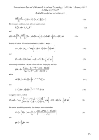
The boundary conditions (6a) – (6c) are used to obtain
  N
1N1
ZPz,0R 
 (12)
and
                
 



 

0 00
1 ,,,0 dxxzxRdxxxQqdxxzxQ
z
pzq
zQ  (13)
Solving the partial differential equations (10) and (11), we get
       





 
x
N
N drrxzXZPzxR
0
211 1exp,  (14)
and
         





 
x
drrxzXzQzxQ
0
3 1exp,0,  (15)
Substituting values from (14) and (15) in (13) and simplifying, we have
 
    
      zzXSqpq
zXDzzP
zQ
N




1*
1*
,0
3
2
1
110


(16)
where
      
 dttdezXD tzX




0
1
2
2
1* 
 (17a)
and
      
 dttsezXS tzX




0
1
2
3
1* 
 (17b)
Using (16) in (15), we find
      
     
     













 
xN
drrxzX
zzXSqpz
zXDz
zPzxQ
0
3
3
2
10 1exp
1*
1*1
, 


 (18)
The partial probability generating functions are hence obtained as
        
 










0
2
0
2
1
1
1*1
,
zX
zXD
zPdxzxRzR N 


(19)
and
   


0
, dxzxQzQ
International Journal of Research in Advent Technology, Vol.7, No.1, January 2019
E-ISSN: 2321-9637
Available online at www.ijrat.org
277
    
     
   
  
















zX
zXS
zXSqpz
zXDz
zP
N
1
1*1
1*
1*1 3
3
2
0
2
1 




(20)
Therefore, the p.g.f. of queue size under steady-state is obtained as
       zRzQzPzn 
    
 








zX
zXDz
z
z NN
1
1*1
1
1 2
2
1 


         
          0
3
32
3
1
1*1
1*11*1
P
zzXSqpzzX
zXSzXdzz N










(21)
To evaluate P0, we use the normalizing condition   11  to yield
   
              DEXENSEDENSEXEq
SEXEq
P
2113
3
0




 (22)
By differentiating equation (21) with respect to z and then evaluating at z = 1, we obtain the mean number of customers in
the system under steady state as
     
              








DEXENSEDENSEXEq
SEXEq
L
2113
3
1


 .
           
 







 


XE
DEXEDEXE
DE
NNN
222
12
2
1 2
1
2
21
1


      
            DEXENNNSEXE
SEXEqXE
2
3
1
121
2






                 DEXENDEXEDEXEDEXE 22
2
2
222
2   .
                     2
3
2
1222
3
2
3
SEXEqXE
SEXESEXESEXE




 .
                   XEXESEXEqDEXENSEXE  2
32 
                   










 SEXESEXESEXESEXEPXE 3
2
3
222
332 
……………………(23)
4. IDLE PERIOD
The idle period of the machining system under
consideration can be expressed as the sum of the
buildup period and setup period. Assuming that vacation
begins at the end of each busy period, the model can be
visualized as a vacation model. The basic purpose is to
utilize the idle time for other operations. For exponential
repair time, E(S) = 1/µ which substituted in (21) yields
International Journal of Research in Advent Technology, Vol.7, No.1, January 2019
E-ISSN: 2321-9637
Available online at www.ijrat.org
278
 
 
         





















 




 

DEXEN
µ
DEN
•
XEq
•
XEq
z
2
1
13
3


 .
    
 
    
     












 
µzXzµqpz
zXDzz
zX
zXDz
z
z NNN
1
1*
1
1*1
1
1
3
2
1
1
2
2
1






……………………(24)
Applying lim µ in (24), we have
      
   
  sayzH
DENzX
zXDz
z
z
z
NN
µ



















1
2
2
1 1
1
1*1
1
1
lim




 (25)
From equation (25), we note that H(z) represent the p.g.f. of additional queue size distribution due to typical
vacation period composed of a buildup period and a random setup period.
Define B0 = length of buildup period; and D0 = length of setup period
Then   







N
BE 0 and    DEDE 0
Since B0 and D0 together define a vacation cycle, we can write
   
     
 say
DE
N
N
DEBE
BE
B 

















00
0
0Pr (26a)
and
     
 







 1Pr1Pr 00
DE
N
DE
BD

(26b)
Rewriting equation (25), we get
 
   
 
 
    
     


























































zXDE
zXDz
DEN
DE
zN
z
DEN
N
z
NN
1
1*1
1
1
2
2
11
1





     zB1zA NN  (27)
where  
 
      
     
















zXDE
zXDz
zBand
zN
z
zA
N
N
N
N
1
1*1
;
1
1
2
2


Clearly, AN(z) and (BN(z)) are the p.g.f.s of the conditional distribution of the number of failed units arriving
during a buildup period and residual life of a setup period respectively, given that the system is idle.
International Journal of Research in Advent Technology, Vol.7, No.1, January 2019
E-ISSN: 2321-9637
Available online at www.ijrat.org
279
Equation (27) clearly states that the additional queue
size distribution due to vacation period of the batch
arrival M/G/1 machining system with different arrival
rates is the convex combination of queue sizes due to
buildup period and setup period.
5. WAITING TIME
We consider all the situations that an arbitrary
(tagged) failed unit can experience. We start by
evaluating the probabilities that a failed unit arrives
during the buildup, setup or busy period.
Denote I = Length of the buildup period
B = Length of the busy period
Then,   






1
N
IE (28)
The p.g.f.  z of the number of failed units waiting for repair when the busy period begins is the sum of N
failed units arrived during buildup and the number of arrivals during setup period.
Hence,      zX1*Dzz 2
N
 (29)
Defining  *B as Laplace-Stieltjes transform of the busy period in M/G/1 queue with Bernoulli feedback, the
busy period B of the machining system under consideration would have the Laplace-Stieltjes transform    *B .
With     DEXEN 2 failed units on the average, the mean busy period E(B) assumes the form
           
    








 SEXEq
SEDEXEN
B
d
d
BE
3
2
0
*



 
(30)
Expected length of a cycle        BEDEIECE  .
Using the renewal reward theorem, we obtain
Pr(System is under buildup period) =
 
 CE
IE
    
              DEXENSEDENSEXEq
SEXEqN
2113
3




 (31a)
Pr(System is under setup period) =
 
 CE
DE
      
              DEXENSEDENSEXEq
SEXEqDE
2113
31




 (31b)
Pr(System is under busy period) =
 
 CE
BE
      
              DEXENSEDENSEXEq
SEXEqSE
2113
21




 (31c)
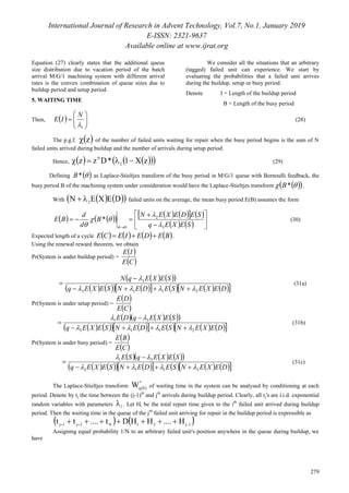
The Laplace-Stieltjes transform  
*
q
W  of waiting time in the system can be analysed by conditioning at each
period. Denote by tj the time between the (j-1)th
and jth
arrivals during buildup period. Clearly, all tj's are i.i.d. exponential
random variables with parameters 1 . Let Hi be the total repair time given to the ith
failed unit arrived during buildup
period. Then the waiting time in the queue of the jth
failed unit arriving for repair in the buildup period is expressible as
   1j21N2j1j H....HHDt....tt  
Assigning equal probability 1/N to an arbitrary failed unit's position anywhere in the queue during buildup, we
have
International Journal of Research in Advent Technology, Vol.7, No.1, January 2019
E-ISSN: 2321-9637
Available online at www.ijrat.org
280
qW ( /arrival during buildup) =    
 
1
1 1
1
*1
*
*
1


















jjN
N
j pS
qS
D
N 




 
 
 
 
 








*
*1
*
1
*
1
1
1
*
1
1
D
pS
qS
pS
qS
N
NN










































 (32)
The conditional mean waiting time is given by
E(Wq/arrival during buildup period)   0
*
/ 
 


buildupduringarrivalW
d
d
q
         
   11
222
1
1 12
221
2
1


 Sq
qSqESEp
q
SEN
DE










 (33)
The waiting time of an arbitrary failed unit arriving during the setup period comprises of three parts –
(i) Time to serve N failed units arriving during buildup period
(ii) Remaining setup time from the epoch at which failed unit arrived.
(iii) Time to serve those failed units who arrived during setup period before it.
The conditional Laplace-Stieltjes transform is given by:





 
yDduringarrivalsn
y,Datarrivalcustomertaggedx,Dperiod,setupatarrival

qW
   yS
nN
 

exp*
Unconditioning {D=x}, {arbitrary failed unit arrived at D – y}, {n arrivals during D – y},
 periodsetupduringarrival
qW
 
 
   
 
 
     
  





























































*1
*1
*
*1
*1
*
*1
*
2
2
pS
S
XEDE
D
pS
S
XED
pS
qS
N
(34)
The conditional mean is then obtained as
          
 qDE
SEXEqDE
q
SNE
periodsetupduringarrivalWE q
2
2
2


      
    








SEXEq
SqESEp
q
XE
2
22
2 2
2 

(35)
For the waiting of a tagged failed unit arriving during the busy period, we consider the busy period as a delayed
cycle for which initial delay is the service time to serve total (N+X) failed units. Here X is the number of arrivals during
setup period with p.g.f.    zXD 1* 2 . Therefore,
 periodbusyduringarrivalWq *
   
      
 
 
   
 
   
  



























































*1
*1
*1
*1
*
*1
*
1
3
2
2
3
pS
S
XE
pS
S
XED
pS
qS
DEXENSE
SEXEq
N
(36)
The conditional mean value is
International Journal of Research in Advent Technology, Vol.7, No.1, January 2019
E-ISSN: 2321-9637
Available online at www.ijrat.org
281
       
      








SEXEqSE
SqESEp
WE q
3
22
2
2
periodbusyatarrival

            
     








DEXENq
DEXEDEXENNN
SE
2
222
22
2
21


(37)
Eqs. (31)-(37) are employed using the total probability arguments to obtain the Laplace-Stieltjes transform of an
arbitrary failed unit's waiting time as :
     
              








DEXENSEDENSEXq
SEXEq
Wq
2113
3*



×  
 
 
 
 

























































*1
*
*1
*
*
1
1
1
1
pS
qS
pS
qS
D
NN
 
 
   
 
 
   
  
























































*1
*1
*
*1
*1
*
*1
*
2
2
2
pS
S
XE
D
pS
S
XED
pS
qS
N
 
 
   
 
   
  































































*1
*1
*1
*1
*
*1
*
1
3
2
3
pS
S
XE
pS
S
XED
pS
qS
N
(38)
The corresponding mean value is obtained as:
     















q
SEN
DEWE q
1
1
2
1

=
    
              







DEXENSEDENSEXEq
SEXEqN
2113
3


×
        
 
      
    


















SEXEq
SqESEp
q
XE
qDE
SEXEqDE
q
SNE
2
22
22
2
2
22 

=
      
              







DEXENSEDENSEXEq
SEXEqDE
2113
31


×
    
      











SEXEqSE
SqESEp
3
22
2
2

            
     












DEXEN
DEXEDEXENNN
q
SE
2
222
2221
2 

.
×
      
              







DEXENSEDENSEXEq
DEXENSE
2113
21


(39)
6. OPTIMAL N-POLICY
International Journal of Research in Advent Technology, Vol.7, No.1, January 2019
E-ISSN: 2321-9637
Available online at www.ijrat.org
282
We propose an optimal N-policy to minimize the mean cost per unit time. First we develop the mathematical
expression for the mean cost per unit time.
There are two kinds of costs, setup cost and failed unit holding cost. In a cycle we incur setup cost Cs once. Let
Ch be the holding cost of a failed unit per unit time in the system. Then, expected total cost per unit time is expressed as
E(TC) =
   
cycleaoflengthMean
costSetupcycleaincostholdingveaccumulatiMean 
(40)
The expected holding cost during buildup period is calculated as
 
hh C
NNN
C
1111 2
11
......
21







 
 (41)
Let Yj be the arrival epoch of the jth
failed unit during setup period and fj(t) be the p.d.f. of the period unit jth
arrival
assumed to be Erlangian  2,j  . Then we formulate the holding cost during setup period for Yj < D as follows.
      











 



 1 01 j
D
jh
j
jh dttftDECYDEC
    





  


D
j
jh dttfDEC
0 1
1
    





 
D
h dtXEtDEC
0
2
   
2
2
2 DEXECh
 (42)
Consequently, the holding cost during setup period is given by
      hCDNE
DEXE







2
2
2
(43)
The term NE(D)Ch originates from the failed units who arrived during the buildup period.
For calculating the holding cost during busy period we start with N failed units (arrived during buildup period)
plus those who arrived during setup period (denoted by Y). Then the accumulated holding cost hn during the busy period
when the server becomes busy with n failed units is.
          
  












 122
1
1
22
SEXEn
SnE
SEnnC
h h
n where  SE (44)
Since the busy period starts with (N+Y) failed units in the model under investigation where Y has p.g.f.
   ZXXDx
12 ,
 
   
     
q
SEYNYNE
SEXEq
qC
hE h
YN


 


2
1
3
      
    
      
     














SEXEq
SEXESE
SEXEq
SEXE
NYE
3
3
3
22
3 1
2 



   
               





 


q
SEDEXEDEXENNN
SEXEq
qCh
2
121 222
22
3


         
    
      
    SEXEq
SEXESE
SEXEq
SEXE
NDEXE
3
3
3
22
3
2
1
2 













 (45)
Therefore, the expected total cost per unit time assumes the form
International Journal of Research in Advent Technology, Vol.7, No.1, January 2019
E-ISSN: 2321-9637
Available online at www.ijrat.org
283
 
         
 CE
ChECDNE
DEXECNN
TCE
sYNh
h










22
1 2
2
1


(46)
Considering N as a continuous variable, we set
  0


N
TCE
which provides optimal value of N as N*
. If N*
is
not an integral value, it can be rounded off to the best possible integral value.
7. CONCLUDING REMARKS
Apart from interest from the point of view of
theoretical structures, bulk arrival queues have been
used for modeling in various situations. Ships arriving at
a port in convoy, mail bags arriving at a central sorting
station are some examples of arrivals in batches of fixed
or random size. Similarly, retrial queues with Bernoulli
feedback have been widely used to model problems in
telephone switching systems, telecommunication
networks and computer networks.
In this paper, we have suggested an optimal N-
policy for MX
/G/1 machining system with Bernoulli
feedback, state-dependent rates and general setup time.
Supplementary variable technique has been employed to
establish the state equations of the model.
By suitable selecting an optimal value of the
decision variable N, the total system cost can be
minimized. The work done can provide valuable insight
to maintainability engineers for designing cost-effective
and efficient models of real time systems arising in the
fields of telecommunication, data communications,
manufacturing systems etc.
REFERENCES
[1] Disney, R.L., McNickle, D.G. and Simon,
B.(1980): The M/G/1 queue with instantaneous
Bernoulli feedback, Nay. Res. Log. Quart.,Vol. 27,
pp. 63 5-644.
[2] Simon, B. (1984): Priority queues with feedback, 3.
ACM, Vol. 31, pp. 134-149.
[3] Rege, K. (1993): On the M/G/l queue with
Bernoulli feedback, Oper. Res. Letters, Vol. 14(3),
pp. 163-170.
[4] Krishna Kumar, B., Arivudainambi, D.and
Vijaykumar, A. (2002) : On the N-policy of M/G/1
feedback queue with varying arrival rates,
OPSEARCH, Vol. 39 (5 & 6), pp. 296-314.
[5] Atencia, I and Moreno, P.(2004): Discrete time
Geo(X)
/GH/I retrial queue with Bernoulli feedback,
Comput. Math. Appl., Vol. 47(8-9), pp. 1273-1294.
[6] Burke P.J.(1975): Delays in single server queues
with batch input, Oper. Res., Vol. 23, pp. 830-833.
[7] Chaudhary, M.L. and Templeton, J.G.C.(1983): A
First Course in Bulk Queues, Wiley, New York.
[8] Lee, H.W. and Lee, S.S.(1991): A batch arrival
queue with different vacations, Comput. Oper. Res.,
Vol. 18(1), pp. 51-58.
[9] Lee, S.S., Lee, H.W., Yoon, S.H. and Chae, K.C.
(1995): Batch arrival queues with N-policy and
single vacation, Comput. Oper. Res, Vol. 22(2), pp.
173-189.
[10]Yue, D.and Cao, J.(1997): Reliability analysis of a
MX
1/MX
2/G1,G2/1 Queucing System with a
repairable service station, Microelectron. Reliab.,
Vol. 37(8), pp. 1225-1231.
[11]Lee, H.W., Park, J.G., Kim, B.K.,Voon, S.H., Aha,
B.Y. and Park, N.I. (1998) : Queue length and
waiting time analysis of a batch arrival queue with
bilevel control, Comput. Oper. Res. Soc., Vol. 25,
Pp. 191-205.
[12]Bacot, J.B. and Dshalalow, J.H.(2001): A bulk
input queueing system with batch gated service and
multiple vacation policy. Math. Comput. Moddel.,
Vol. 34(7-8), pp. 873-886.
[13]Chaudhary, G.and Paul, M.(2004): A batch arrival
queue with an additional service channel under N-
policy, Appl. Math. Comput.,Vol. 156 (1), pp. 115-
130.

Paper id 71201933

  • 1.
    International Journal ofResearch in Advent Technology, Vol.7, No.1, January 2019 E-ISSN: 2321-9637 Available online at www.ijrat.org 273 Optimal N-Policy for Bernoulli feedback Mx /G/1 Machining System Krishna Gopal Varshney, Dr.Rajvir Singh (1) Departments of Mathematics, Government Degree College,Kasganj (U.P.) (Affiliated to Dr.B.R. Ambedkar University Agra) (2) Basic Education Department, Mainpuri (U.P.) E-mail : kgp123mayanath@gmail.com, rajshakya1582@gmail.com Abstract- This study applies N-policy to an MX /G/1 repairable machining system with Bernoulli feedback and general setup time. The arrival rate of the failed units depends on the state of the system which may be in buildup, setup and busy states. Supplementary variable technique is employed to obtain the probability generating function for the system queue size distribution and the mean number of failed units in the system under steady state conditions. The Laplace-Stieltjes transform of the waiting time is obtained which is further used to evaluate its mean value. The total operational cost of the system is minimized in order to determine the optimal value of N. Keywords: N-Policy, MX /G/1 system, Batch arrival, Bernoulli feedback, Setup time, Supplementary variable technique, Queue size, waiting time. 1. INTRODUCTION Queueing theory has emerged as one of the foremost areas of research because of its utility in simulating many real life systems.we proposed an optimal control N-policy for an M/Ek/1 system. We now shift our focus to a batch failure queueing model with feedback. Many congestion situations arising in data communication and telecommunication systems can be modeled as feedback queueing models where a unit receiving incomplete service may repeatedly seek service till its service is completed. In recent past, queueing systems with Bernoulli feedback have been extensively investigated by Disney et al. (1980), Simon (1984) and many others. An M/G/1 queue with Bernoulli feedback was studied by Rege (1993). Retrial queues with Bernoulli feedback have been analysed by Krishna Kumar et al. (2002) and recently by Atencia and Moreno (2004). In many realistic situations, customers arrive in batches. Burke (1975) and Chaudhary and Templeton (1983) have contributed significantly to the study the bulk arrival queues. Lee and Lee (1991) examined an M/G/1 batch arrival queue with different server vacations. Batch arrival queues have been thoroughly investigated by Lee et al. (1995), Yue and Cao (1997), Lee et al. (1998), Bacot and Dshalalow (2001) and others. Chaudhary and Paul (2004) implemented an N- policy to a batch arrival queue with additional service channel. The purpose of this paper is to investigate an optimal N-policy for an M/G/1 batch failure of units of multi-component machining system with Bernoulli feedback and state-dependent failure rates. At any time, the system can be in buildup, setup or busy states. We assume that the failed unit having received partial repair, rejoins at the head of the queue and hence assumes priority over the other failed units whose repair is yet to commence. The rest of the paper is organized as follows: In section 2, the system under investigation is described along with requisite notations. Supplementary variable technique is employed in section 3 to establish the state equations and obtain the steady-state queue length. Section 4 covers the queue size distribution during an idle period. We obtain the Laplace-Stieltjes transform of the stationary waiting time of an arbitrary failed unit in the system in the next section 5. The total operating cost of the system is formulated as a function of N in section 6 to determine the optimal value of N. We conclude our investigation in section 7 with concluding remarks. 2. MODEL DESCRIPTION AND NOTATIONS We study an MX /G/1 machining system with Bernoulli feedback and set up times under N-policy. The underlying assumptions governing the machining system are: (i) The life-time of units is considered to be exponential distributed. For repair of failed units, we assume i.i.d. general distribution. (ii) The failed units arrive in batch of random size to a machining centre having single server who repairs these units according to FCFS rule. (iii) The arrival rate of the failed units depends on the state of the system which may be in buildup, setup or busy states. Accordingly the arrival rate is ,,, 321  respectively.
  • 2.
    International Journal ofResearch in Advent Technology, Vol.7, No.1, January 2019 E-ISSN: 2321-9637 Available online at www.ijrat.org 274 (iv) The buildup period comprises of the time during which the server is idle until N failed units accumulate in the system. (v) The server initiates the setup as soon as the number of failed units reaches N. The setup period is general distributed and is independent of other random variables involved. (vi) At the end of the setup period, the server starts providing exhaustive repair of failed units till the system again becomes empty. This is called the busy period. (vii) If repair of a failed unit is not completed successfully, it rejoins the queue for repair. However other failed units leave the system after getting repair. The following notations are used to completely specify the queueing system: X : Random variable denoting the batch size X(z) : p.g.f. of the batch size X S : Random variable for the repair of the failed units s(x) : p.d.f. of S S*( ) : Laplace transform of s(x) D : Random variable for setup time d(x) : p.d.f. of D D*( ) : Laplace transform of d(x) p,q : Probability that a failed unit is feedback to the head of the queue for retrial and probability that the failed unit departs from the system after completion of repair, respectively, (p+q = 1) Pn : Pr (System is in buildup period and there are n failed units in the system under steady- state), n = 0, 1, 2, ....., N-1 Rn(x)dx : Pr (System is in setup period, there are n failed units in the system under steady state and elapsed setup time lies in (x, (x+ ∆x)), n = N, N +1, N + 2, N+3, .................. Qn(x)dx : Pr (Server is busy, there are n failed units in the system under steady state and elapsed repair time of the failed unit currently being repaired lies in (x,( x _ ∆x)), n = 1, 2, 3, .....  x : Conditional completion rates at time x for setup time µ(x) : Conditional completion rates at time x for repair P(z) : p.g.f. or Pn R(x,z) : p.g.f. of Rn(x) Q(x,z) : p.g.f. of Qn(x)  z : p.g.f. of system size at an arbitrary epoch under steady-state  * H : Laplace-Stieltjes transform of p.d.f. of total repair time H(t) 3. QUEUE SIZE DISTRIBUTION The elapsed repair time and elapsed setup time are treated as supplementary variables. Assuming steady state, the stationary state equations are formulated as: 1n1n1 PP0  , n = 1, 2, 3, …….. N-1 (1)       xRx dx xdR N N   2 (2)
  • 3.
    International Journal ofResearch in Advent Technology, Vol.7, No.1, January 2019 E-ISSN: 2321-9637 Available online at www.ijrat.org 275                1 1 22 . n k knn n kXprobxRxRx dx xdR  1 Nn (3)       xQxµ dx xdQ 13 1   (4)           kXprobxQxQxµ dx xdQ n k knn n      . 1 1 33  n = 2,3,4, ..... (5) In fact,            xS xs x xD xd x     1 , 1  The boundary conditions for the state equations are given by     1Nn,00R,P0R n1N1N   (6a)                0 0 1 1,....2,1,0 NndxxxQpdxxxQqQ nnn  (6b)                      0 0 0 1 ,0 dxxxRdxxxQpdxxxQqQ nnnn  n = N, N + 1, N + 2,.. (6c) The normalizing conditions is                 N n n nn Nn n dxxxQdxxxRP 0 0 1 0 1 (7) Define probability generating functions as       1 0 N n n n ZPzP (8a)        Nn n n zxRzxR , (8b)        Nn n n zxQzxQ , (8c)        zRzQzPz  (8d) Now multiplying eq. (1) by zn and summing, we have   z1 z1 PzP N 0    (9) Multiplying eqs. (2) and (3) with appropriate powers of zn and summing, we get          zxRxzX x zxR ,1 , 2     (10) In like manner, eqs. (4) and (5) yield :
  • 4.
    International Journal ofResearch in Advent Technology, Vol.7, No.1, January 2019 E-ISSN: 2321-9637 Available online at www.ijrat.org 276          zxQxzX x zxQ ,1 , 3     (11) The boundary conditions (6a) – (6c) are used to obtain   N 1N1 ZPz,0R   (12) and                          0 00 1 ,,,0 dxxzxRdxxxQqdxxzxQ z pzq zQ  (13) Solving the partial differential equations (10) and (11), we get                x N N drrxzXZPzxR 0 211 1exp,  (14) and                  x drrxzXzQzxQ 0 3 1exp,0,  (15) Substituting values from (14) and (15) in (13) and simplifying, we have              zzXSqpq zXDzzP zQ N     1* 1* ,0 3 2 1 110   (16) where         dttdezXD tzX     0 1 2 2 1*   (17a) and         dttsezXS tzX     0 1 2 3 1*   (17b) Using (16) in (15), we find                                   xN drrxzX zzXSqpz zXDz zPzxQ 0 3 3 2 10 1exp 1* 1*1 ,     (18) The partial probability generating functions are hence obtained as                      0 2 0 2 1 1 1*1 , zX zXD zPdxzxRzR N    (19) and       0 , dxzxQzQ
  • 5.
    International Journal ofResearch in Advent Technology, Vol.7, No.1, January 2019 E-ISSN: 2321-9637 Available online at www.ijrat.org 277                                   zX zXS zXSqpz zXDz zP N 1 1*1 1* 1*1 3 3 2 0 2 1      (20) Therefore, the p.g.f. of queue size under steady-state is obtained as        zRzQzPzn                 zX zXDz z z NN 1 1*1 1 1 2 2 1                        0 3 32 3 1 1*1 1*11*1 P zzXSqpzzX zXSzXdzz N           (21) To evaluate P0, we use the normalizing condition   11  to yield                   DEXENSEDENSEXEq SEXEq P 2113 3 0      (22) By differentiating equation (21) with respect to z and then evaluating at z = 1, we obtain the mean number of customers in the system under steady state as                              DEXENSEDENSEXEq SEXEq L 2113 3 1    .                          XE DEXEDEXE DE NNN 222 12 2 1 2 1 2 21 1                      DEXENNNSEXE SEXEqXE 2 3 1 121 2                        DEXENDEXEDEXEDEXE 22 2 2 222 2   .                      2 3 2 1222 3 2 3 SEXEqXE SEXESEXESEXE      .                    XEXESEXEqDEXENSEXE  2 32                                 SEXESEXESEXESEXEPXE 3 2 3 222 332  ……………………(23) 4. IDLE PERIOD The idle period of the machining system under consideration can be expressed as the sum of the buildup period and setup period. Assuming that vacation begins at the end of each busy period, the model can be visualized as a vacation model. The basic purpose is to utilize the idle time for other operations. For exponential repair time, E(S) = 1/µ which substituted in (21) yields
  • 6.
    International Journal ofResearch in Advent Technology, Vol.7, No.1, January 2019 E-ISSN: 2321-9637 Available online at www.ijrat.org 278                                             DEXEN µ DEN • XEq • XEq z 2 1 13 3    .                                 µzXzµqpz zXDzz zX zXDz z z NNN 1 1* 1 1*1 1 1 3 2 1 1 2 2 1       ……………………(24) Applying lim µ in (24), we have              sayzH DENzX zXDz z z z NN µ                    1 2 2 1 1 1 1*1 1 1 lim      (25) From equation (25), we note that H(z) represent the p.g.f. of additional queue size distribution due to typical vacation period composed of a buildup period and a random setup period. Define B0 = length of buildup period; and D0 = length of setup period Then           N BE 0 and    DEDE 0 Since B0 and D0 together define a vacation cycle, we can write            say DE N N DEBE BE B                   00 0 0Pr (26a) and                 1Pr1Pr 00 DE N DE BD  (26b) Rewriting equation (25), we get                                                                                zXDE zXDz DEN DE zN z DEN N z NN 1 1*1 1 1 2 2 11 1           zB1zA NN  (27) where                                  zXDE zXDz zBand zN z zA N N N N 1 1*1 ; 1 1 2 2   Clearly, AN(z) and (BN(z)) are the p.g.f.s of the conditional distribution of the number of failed units arriving during a buildup period and residual life of a setup period respectively, given that the system is idle.
  • 7.
    International Journal ofResearch in Advent Technology, Vol.7, No.1, January 2019 E-ISSN: 2321-9637 Available online at www.ijrat.org 279 Equation (27) clearly states that the additional queue size distribution due to vacation period of the batch arrival M/G/1 machining system with different arrival rates is the convex combination of queue sizes due to buildup period and setup period. 5. WAITING TIME We consider all the situations that an arbitrary (tagged) failed unit can experience. We start by evaluating the probabilities that a failed unit arrives during the buildup, setup or busy period. Denote I = Length of the buildup period B = Length of the busy period Then,          1 N IE (28) The p.g.f.  z of the number of failed units waiting for repair when the busy period begins is the sum of N failed units arrived during buildup and the number of arrivals during setup period. Hence,      zX1*Dzz 2 N  (29) Defining  *B as Laplace-Stieltjes transform of the busy period in M/G/1 queue with Bernoulli feedback, the busy period B of the machining system under consideration would have the Laplace-Stieltjes transform    *B . With     DEXEN 2 failed units on the average, the mean busy period E(B) assumes the form                           SEXEq SEDEXEN B d d BE 3 2 0 *      (30) Expected length of a cycle        BEDEIECE  . Using the renewal reward theorem, we obtain Pr(System is under buildup period) =    CE IE                    DEXENSEDENSEXEq SEXEqN 2113 3      (31a) Pr(System is under setup period) =    CE DE                      DEXENSEDENSEXEq SEXEqDE 2113 31      (31b) Pr(System is under busy period) =    CE BE                      DEXENSEDENSEXEq SEXEqSE 2113 21      (31c) The Laplace-Stieltjes transform   * q W  of waiting time in the system can be analysed by conditioning at each period. Denote by tj the time between the (j-1)th and jth arrivals during buildup period. Clearly, all tj's are i.i.d. exponential random variables with parameters 1 . Let Hi be the total repair time given to the ith failed unit arrived during buildup period. Then the waiting time in the queue of the jth failed unit arriving for repair in the buildup period is expressible as    1j21N2j1j H....HHDt....tt   Assigning equal probability 1/N to an arbitrary failed unit's position anywhere in the queue during buildup, we have
  • 8.
    International Journal ofResearch in Advent Technology, Vol.7, No.1, January 2019 E-ISSN: 2321-9637 Available online at www.ijrat.org 280 qW ( /arrival during buildup) =       1 1 1 1 *1 * * 1                   jjN N j pS qS D N                        * *1 * 1 * 1 1 1 * 1 1 D pS qS pS qS N NN                                            (32) The conditional mean waiting time is given by E(Wq/arrival during buildup period)   0 * /      buildupduringarrivalW d d q              11 222 1 1 12 221 2 1    Sq qSqESEp q SEN DE            (33) The waiting time of an arbitrary failed unit arriving during the setup period comprises of three parts – (i) Time to serve N failed units arriving during buildup period (ii) Remaining setup time from the epoch at which failed unit arrived. (iii) Time to serve those failed units who arrived during setup period before it. The conditional Laplace-Stieltjes transform is given by:        yDduringarrivalsn y,Datarrivalcustomertaggedx,Dperiod,setupatarrival  qW    yS nN    exp* Unconditioning {D=x}, {arbitrary failed unit arrived at D – y}, {n arrivals during D – y},  periodsetupduringarrival qW                                                                                   *1 *1 * *1 *1 * *1 * 2 2 pS S XEDE D pS S XED pS qS N (34) The conditional mean is then obtained as             qDE SEXEqDE q SNE periodsetupduringarrivalWE q 2 2 2                       SEXEq SqESEp q XE 2 22 2 2 2   (35) For the waiting of a tagged failed unit arriving during the busy period, we consider the busy period as a delayed cycle for which initial delay is the service time to serve total (N+X) failed units. Here X is the number of arrivals during setup period with p.g.f.    zXD 1* 2 . Therefore,  periodbusyduringarrivalWq *                                                                                        *1 *1 *1 *1 * *1 * 1 3 2 2 3 pS S XE pS S XED pS qS DEXENSE SEXEq N (36) The conditional mean value is
  • 9.
    International Journal ofResearch in Advent Technology, Vol.7, No.1, January 2019 E-ISSN: 2321-9637 Available online at www.ijrat.org 281                        SEXEqSE SqESEp WE q 3 22 2 2 periodbusyatarrival                             DEXENq DEXEDEXENNN SE 2 222 22 2 21   (37) Eqs. (31)-(37) are employed using the total probability arguments to obtain the Laplace-Stieltjes transform of an arbitrary failed unit's waiting time as :                              DEXENSEDENSEXq SEXEq Wq 2113 3*    ×                                                                    *1 * *1 * * 1 1 1 1 pS qS pS qS D NN                                                                            *1 *1 * *1 *1 * *1 * 2 2 2 pS S XE D pS S XED pS qS N                                                                                 *1 *1 *1 *1 * *1 * 1 3 2 3 pS S XE pS S XED pS qS N (38) The corresponding mean value is obtained as:                      q SEN DEWE q 1 1 2 1  =                            DEXENSEDENSEXEq SEXEqN 2113 3   ×                                          SEXEq SqESEp q XE qDE SEXEqDE q SNE 2 22 22 2 2 22   =                              DEXENSEDENSEXEq SEXEqDE 2113 31   ×                        SEXEqSE SqESEp 3 22 2 2                                 DEXEN DEXEDEXENNN q SE 2 222 2221 2   . ×                              DEXENSEDENSEXEq DEXENSE 2113 21   (39) 6. OPTIMAL N-POLICY
  • 10.
    International Journal ofResearch in Advent Technology, Vol.7, No.1, January 2019 E-ISSN: 2321-9637 Available online at www.ijrat.org 282 We propose an optimal N-policy to minimize the mean cost per unit time. First we develop the mathematical expression for the mean cost per unit time. There are two kinds of costs, setup cost and failed unit holding cost. In a cycle we incur setup cost Cs once. Let Ch be the holding cost of a failed unit per unit time in the system. Then, expected total cost per unit time is expressed as E(TC) =     cycleaoflengthMean costSetupcycleaincostholdingveaccumulatiMean  (40) The expected holding cost during buildup period is calculated as   hh C NNN C 1111 2 11 ...... 21           (41) Let Yj be the arrival epoch of the jth failed unit during setup period and fj(t) be the p.d.f. of the period unit jth arrival assumed to be Erlangian  2,j  . Then we formulate the holding cost during setup period for Yj < D as follows.                         1 01 j D jh j jh dttftDECYDEC                D j jh dttfDEC 0 1 1             D h dtXEtDEC 0 2     2 2 2 DEXECh  (42) Consequently, the holding cost during setup period is given by       hCDNE DEXE        2 2 2 (43) The term NE(D)Ch originates from the failed units who arrived during the buildup period. For calculating the holding cost during busy period we start with N failed units (arrived during buildup period) plus those who arrived during setup period (denoted by Y). Then the accumulated holding cost hn during the busy period when the server becomes busy with n failed units is.                            122 1 1 22 SEXEn SnE SEnnC h h n where  SE (44) Since the busy period starts with (N+Y) failed units in the model under investigation where Y has p.g.f.    ZXXDx 12 ,             q SEYNYNE SEXEq qC hE h YN       2 1 3                                        SEXEq SEXESE SEXEq SEXE NYE 3 3 3 22 3 1 2                                  q SEDEXEDEXENNN SEXEq qCh 2 121 222 22 3                             SEXEq SEXESE SEXEq SEXE NDEXE 3 3 3 22 3 2 1 2                (45) Therefore, the expected total cost per unit time assumes the form
  • 11.
    International Journal ofResearch in Advent Technology, Vol.7, No.1, January 2019 E-ISSN: 2321-9637 Available online at www.ijrat.org 283              CE ChECDNE DEXECNN TCE sYNh h           22 1 2 2 1   (46) Considering N as a continuous variable, we set   0   N TCE which provides optimal value of N as N* . If N* is not an integral value, it can be rounded off to the best possible integral value. 7. CONCLUDING REMARKS Apart from interest from the point of view of theoretical structures, bulk arrival queues have been used for modeling in various situations. Ships arriving at a port in convoy, mail bags arriving at a central sorting station are some examples of arrivals in batches of fixed or random size. Similarly, retrial queues with Bernoulli feedback have been widely used to model problems in telephone switching systems, telecommunication networks and computer networks. In this paper, we have suggested an optimal N- policy for MX /G/1 machining system with Bernoulli feedback, state-dependent rates and general setup time. Supplementary variable technique has been employed to establish the state equations of the model. By suitable selecting an optimal value of the decision variable N, the total system cost can be minimized. The work done can provide valuable insight to maintainability engineers for designing cost-effective and efficient models of real time systems arising in the fields of telecommunication, data communications, manufacturing systems etc. REFERENCES [1] Disney, R.L., McNickle, D.G. and Simon, B.(1980): The M/G/1 queue with instantaneous Bernoulli feedback, Nay. Res. Log. Quart.,Vol. 27, pp. 63 5-644. [2] Simon, B. (1984): Priority queues with feedback, 3. ACM, Vol. 31, pp. 134-149. [3] Rege, K. (1993): On the M/G/l queue with Bernoulli feedback, Oper. Res. Letters, Vol. 14(3), pp. 163-170. [4] Krishna Kumar, B., Arivudainambi, D.and Vijaykumar, A. (2002) : On the N-policy of M/G/1 feedback queue with varying arrival rates, OPSEARCH, Vol. 39 (5 & 6), pp. 296-314. [5] Atencia, I and Moreno, P.(2004): Discrete time Geo(X) /GH/I retrial queue with Bernoulli feedback, Comput. Math. Appl., Vol. 47(8-9), pp. 1273-1294. [6] Burke P.J.(1975): Delays in single server queues with batch input, Oper. Res., Vol. 23, pp. 830-833. [7] Chaudhary, M.L. and Templeton, J.G.C.(1983): A First Course in Bulk Queues, Wiley, New York. [8] Lee, H.W. and Lee, S.S.(1991): A batch arrival queue with different vacations, Comput. Oper. Res., Vol. 18(1), pp. 51-58. [9] Lee, S.S., Lee, H.W., Yoon, S.H. and Chae, K.C. (1995): Batch arrival queues with N-policy and single vacation, Comput. Oper. Res, Vol. 22(2), pp. 173-189. [10]Yue, D.and Cao, J.(1997): Reliability analysis of a MX 1/MX 2/G1,G2/1 Queucing System with a repairable service station, Microelectron. Reliab., Vol. 37(8), pp. 1225-1231. [11]Lee, H.W., Park, J.G., Kim, B.K.,Voon, S.H., Aha, B.Y. and Park, N.I. (1998) : Queue length and waiting time analysis of a batch arrival queue with bilevel control, Comput. Oper. Res. Soc., Vol. 25, Pp. 191-205. [12]Bacot, J.B. and Dshalalow, J.H.(2001): A bulk input queueing system with batch gated service and multiple vacation policy. Math. Comput. Moddel., Vol. 34(7-8), pp. 873-886. [13]Chaudhary, G.and Paul, M.(2004): A batch arrival queue with an additional service channel under N- policy, Appl. Math. Comput.,Vol. 156 (1), pp. 115- 130.