Downloaded 20 times
![Putting the raster max and min elevation in a shapefile
path = "/home/moovida/giscourse/data_1_3/spearfish_elevation/elevation.asc"
dir = new Directory("/home/moovida/giscourse/data_1_3/spearfish_elevation/")
// create the vector layer for the max and min
layer = dir.create('spearfish_max_min',[['geom','Point','epsg:26713'],
['type','string'],['value','double']])
// get max and min from raster
elev = Raster.read(path)
count = 0
min = 10000000; minCol = 0; minRow = 0 // can be put on one line using semicolon
max = 0; maxCol = 0; maxRow = 0
for ( col in 0..(elev.cols-1) ){
for ( row in 0..(elev.rows-1) ){
value = elev.valueAt( col, row )
if(!elev.isNoValue( value )){
if(value > max ) {
max = value
maxCol = col // important, keep also the
maxRow = row // positions of the max and min
}
if(value < min ) {
min = value
minCol = col
minRow = row
}
}
}
}
// get the world position from the raster grid position
minXY = elev.positionAt(minCol, minRow)
maxXY = elev.positionAt(maxCol, maxRow)
// add the features
layer.add([new Point(minXY[0], minXY[1]),'min', min])
layer.add([new Point(maxXY[0], maxXY[1]),'max', max])](https://image.slidesharecdn.com/geographicscriptinginudig-halfwaybetweenuseranddeveloper5-130323001204-phpapp01/85/05-Geographic-scripting-in-uDig-halfway-between-user-and-developer-7-320.jpg)
![Neighbour operations
With the raster object it is possible to access the neighbour cell values. In
this example we will extract pits:
path = "/home/moovida/giscourse/data_1_3/spearfish_elevation/elevation.asc"
dir = new Directory("/home/moovida/giscourse/data_1_3/spearfish_elevation/")
// create the vector layer for the pits
layer = dir.create('spearfish_pits',[['geom','Point','epsg:26713'],
['value','double']])
elev = Raster.read(path)
for ( col in 0..(elev.cols-1) ){
for ( row in 0..(elev.rows-1) ){
value = elev.valueAt( col, row )
if(!elev.isNoValue( value )){
// get all neighbour values
surr = elev.surrounding(col, row)
isPit = true
surr.each(){ neighValue -> // check if one is smaller
if(neighValue <= value ) isPit = false
}
if(isPit){
// add pits to the vector layer
xy = elev.positionAt(col, row)
layer.add([new Point(xy[0], xy[1]), value])
}
}
}
}](https://image.slidesharecdn.com/geographicscriptinginudig-halfwaybetweenuseranddeveloper5-130323001204-phpapp01/85/05-Geographic-scripting-in-uDig-halfway-between-user-and-developer-11-320.jpg)
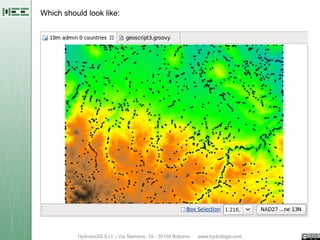
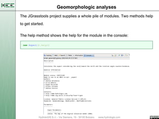
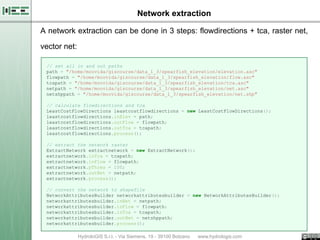


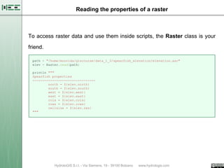
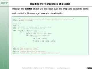
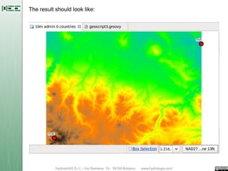
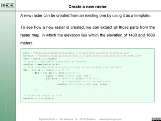
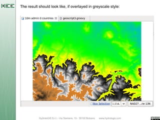
The document discusses using the JGrasstools library within Geoscript to perform geospatial analyses and processing on raster data. It provides examples of reading raster properties, creating new rasters, extracting features like pits and contours, and performing analyses like aspect modeling and network extraction. The library allows accessing the same raster processing modules available in uDig from within Geoscript scripts.