04 Geographic scripting in uDig - halfway between user and developer

Open Source GIS

Geographic scripting in uDig - halfway
between user and developer
Geoinformation Research Group, Department of Geography
University of Potsdam
March 2013

Geoscript
Tutor: Andrea Antonello

ydroloGIS nvironmental ngineering
HydroloGIS S.r.l. - Via Siemens, 19 - 39100 Bolzano www.hydrologis.com

Introduction to Geoscript
Geoscript is a geo processing library that is provided in various scripting

environments and is supported in the uDig scripting editor.

As for every scripting language, modules have to be enabled to be used.

Once one knows the language very well, he can proceed with importing the

necessary modules. The scripting editor has a button that helps by adding

the most used imports.

Most used packages for vector geoscripting

A list of imports and a short description of their purpose:

// most used packages

// handles geometries objects
import geoscript.geom.*
// handles projections
import geoscript.proj.*
// handles rendering and plotting
import geoscript.render.*
// enables layer management
import geoscript.layer.*
// enables tools to work with style
import geoscript.style.*
// handles various viewers
import geoscript.viewer.*
// the package that works with filters
import geoscript.filter.*
// the package that handles workspaces
import geoscript.workspace.*
// support for jgrasstools modules
import org.jgrasstools.modules.*

Building Geometries

Geometries can be built through the use of their constructors:

// build geometries by constructors

// simple geometries
def geom = new Point(30,10)
println geom
geom = new LineString([30,10], [10,30], [20,40], [40,40])
println geom
geom = new Polygon([30,10], [10,20], [20,40], [40,40], [30,10])
println geom
geom = new Polygon([[[35,10],[10,20],[15,40],[45,45],[35,10]],
[[20,30],[35,35],[30,20],[20,30]]])
println geom

// multi-geometries
geom = new MultiPoint([10,40],[40,30],[20,20],[30,10])
println geom
geom = new MultiLineString([[10,10],[20,20],[10,40]],
[[40,40],[30,30],[40,20],[30,10]])
println geom
geom = new MultiPolygon([[[30,20], [10,40], [45,40], [30,20]]],
[[[15,5], [40,10], [10,20], [5,10], [15,5]]])
println geom

or through their well known text representation:

// build geometries by wkt
geom = Geometry.fromWKT("POINT (30 10)")
println geom
geom = Geometry.fromWKT("LINESTRING (30 10, 10 30, 20 40, 40 40)")
println geom
geom = Geometry.fromWKT("POLYGON ((30 10, 10 20, 20 40, 40 40, 30 10))")
println geom
geom = Geometry.fromWKT("POLYGON ((35 10, 10 20, 15 40, 45 45, 35 10), " +
"(20 30, 35 35, 30 20, 20 30))")
println geom
geom = Geometry.fromWKT("MULTIPOINT ((10 40), (40 30), (20 20), (30 10))")
println geom
geom = Geometry.fromWKT("MULTILINESTRING ((10 10, 20 20, 10 40), " +
"(40 40, 30 30, 40 20, 30 10))")
println geom
geom = Geometry.fromWKT("MULTIPOLYGON (((30 20, 10 40, 45 40, 30 20)), " +
"((15 5, 40 10, 10 20, 5 10, 15 5)))")
println geom

A test set of geometries to use as reference

To better explain the various functions and predicates we will start by

creating a set of geometries on which to apply the operations.

You are now able to create the following points, line and polygons:

5
g6
g1
g4

g5
g2
g3
0
0 5

Build the test set

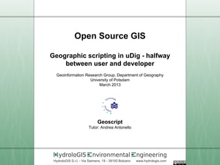
Let's create the geometries that make up the test set:

// build the example dataset
def g1 = Geometry.fromWKT("POLYGON ((0 0, 0 5, 5 5, 5 0, 0 0))")
def g3 = Geometry.fromWKT("POINT (4 1)")
def g4 = Geometry.fromWKT("POINT (5 4)")
def g5 = Geometry.fromWKT("LINESTRING (1 0, 1 6)")

Geoscript has a plotting utility that makes it possible to quickly check:

// plot geometries
Plot.plot([g1, g2, g3, g4, g5, g6])

Predicates

Intersects

Let's see which geometries intersect with g1 and print the result:

println g1.intersects(g2) // true

Note that geometries that touch (like g1 and g2) also intersect.

Touches

Let's test which geometries touch g1 and print the result:

println g1.touches(g2) // true
println g1.touches(g3) // false
println g1.touches(g4) // true

Contains

Let's test which geometries are contained by g1 and print the result:

println g1.contains(g2) // false
println g1.contains(g3) // true

Mind that a point on the border is not contained, so only g3 is contained. This

can be solved through the covers predicate.

Covers

println g1.covers(g2) // false
println g1.covers(g3) // true
println g1.covers(g4) // true

As you can see, now also g4 is covered.

Functions

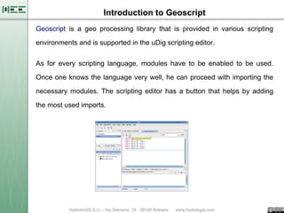
Intersection

// the intersection of polygons returns a polygon
def g1_inter_g6 = g1.intersection(g6)
println g1_inter_g6
Plot.plot([g1_inter_g6, g1, g6])
// but the intersection of touching polygons returns a line
println g1.intersection(g2)
// the intersection of a polygon with a point is a point
// the intersection of a polygon with a line is a point

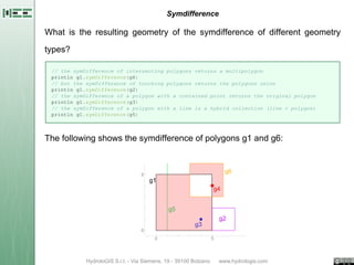
The intersection of polygons g1 and g6:

5
g6
g1
g4

g5
g2
g3
0
0 5

Symdifference

What is the resulting geometry of the symdifference of different geometry

types?

// the symDifference of intersecting polygons returns a multipolygon
println g1.symDifference(g6)
// but the symDifference of touching polygons returns the polygons union
// the symDifference of a polygon with a contained point returns the original polygon
// the symDifference of a polygon with a line is a hybrid collection (line + polygon)

The following shows the symdifference of polygons g1 and g6:

5
g6
g1
g4

g5
g2
g3
0
0 5

Union

What is the resulting geometry of the union of different geometry types?

// the union of intersecting polygons returns a polygon
println g1.union(g6)
// same as the union of touching polygons
// the union of a polygon with a contained point is a point returns the original polygon
// the union of a polygon with a line is a hybrid collection (line + polygon)

The following shows the union of polygons g1 and g6:

5
g6
g1
g4

g5
g2
g3
0
0 5

Difference

The difference of geometries obviously depends on the calling object:

// this returns g1 minus the overlapping part of g6
println g1.difference(g6)
// while this returns g6 minus the overlapping part of g1
// in the case of difference with lines, the result is the original polygon
// with additional points in the intersections
// the difference of polygon and point is the original polygon

The following shows the difference of polygons g1 and g6:

5
g6
g1
g4

g5
g2
g3
0
0 5

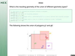
Buffer

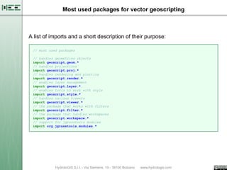
Creating a buffer around a

geometry always generates a

polygon geometry. The behaviour

can be tweaked, depending on the

geometry type:
// the buffer of a point
def b1 = g3.buffer(1.0)

// the buffer of a point with few quandrant segments
def b2 = g3.buffer(1.0, 1)

// round end cap style, few points
def b3 = g5.buffer(1.0, 2, Geometry.CAP_ROUND)

// round end cap style, more points
def b4 = g5.buffer(1.0, 10, Geometry.CAP_ROUND)

// square end cap style
def b5 = g5.buffer(1.0, -1, Geometry.CAP_SQUARE)

// single sided buffer
def b6 = g5.singleSidedBuffer(-0.5)

// plot the geometries
Plot.plot([b6, b5, b4, b3, b2, b1])

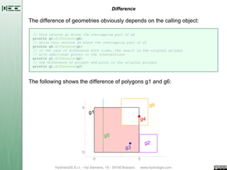
Convex Hull

To test the convext hull operation, let's create a geometry collection

containing the line and all the polygons. Then simply apply the convex hull

function:

// let's create a geometry collection with the polygons and line in it
def collection = new GeometryCollection(g1, g2, g5, g6)
// and apply the convex hull
def convexhull = collection.convexHull
Plot.plot([convexhull, g1, g2, g5, g6])

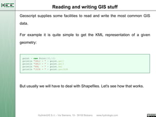
Transformations

def square = new Polygon([[[0,0],[1,0],[1,1],[0,1],[0,0]]])
// scale the sqaure by 4 times
def squareLarge = square.scale(4,4)
// move it by x, y units
def squareTranslate = square.translate(2,2)
// move it and then rotate it by 45 degrees
def squareTranslateRotate = square.translate(2,2).rotate(Math.toRadians(45))
// realize that the order of things are there for a reason
def squareRotateTranslate = square.rotate(Math.toRadians(45)).translate(2,2)
// rotate around a defined center
def squareTranslateRotateCenter = square.translate(2,2).rotate(Math.toRadians(45), 2.5, 2.5)
// shear the square
def squareShear = square.shear(0.75,0)
// check the results
Plot.plot([square, squareLarge, squareTranslate, squareTranslateRotate,
squareRotateTranslate, squareTranslateRotateCenter, squareShear])

Projections

// create a projection object
def latLonPrj = new Projection("epsg:4326")
println latLonPrj.wkt

def latLonPoint = new Point(11, 46)

// transform the point to the new prj
def utm32nPoint = latLonPrj.transform(latLonPoint, "epsg:32632")
println "Transformed ${latLonPoint} to ${utm32nPoint}"

// a simple way to do so is
def utm32nPoint1 = Projection.transform(latLonPoint, 'epsg:4326', 'epsg:32632')
println "Transformed ${latLonPoint} to ${utm32nPoint1}"

// one can also create projections from the wkt representation
def wkt = """GEOGCS["WGS 84",
DATUM["World Geodetic System 1984",
SPHEROID["WGS 84", 6378137.0, 298.257223563, AUTHORITY["EPSG","7030"]],
AUTHORITY["EPSG","6326"]],
PRIMEM["Greenwich", 0.0, AUTHORITY["EPSG","8901"]],
UNIT["degree", 0.017453292519943295],
AXIS["Geodetic longitude", EAST],
AXIS["Geodetic latitude", NORTH],
AUTHORITY["EPSG","4326"]]
"""

def projFromWkt = new Projection(wkt)
def utm32nPoint2 = projFromWkt.transform(latLonPoint, "epsg:32632")
println "Transformed ${latLonPoint} to ${utm32nPoint2}"

Reading and writing GIS stuff
Geoscript supplies some facilities to read and write the most common GIS

data.

For example it is quite simple to get the KML representation of a given

geometry:

point = new Point(30,10)
println "GML2 = " + point.gml2
println "GML3 = " + point.gml3
println "KML = " + point.kml
println "JSON = " + point.geoJSON

But usually we will have to deal with Shapefiles. Let's see how that works.

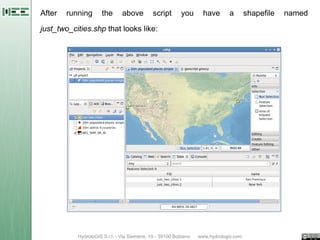
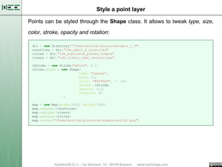
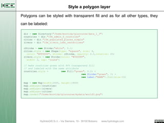
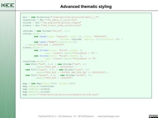
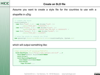
Creating the first shapefile

To create a shapefile, one first has to create a new layer defining the

geometry to use and the attributes to add to each feature.

// define a working folder
Directory dir = new Directory("/home/moovida/giscourse/mydata/")

// create a new layer of points with just one string attribute
def simpleLayer = dir.create('just_two_cities',[['geom','Point','epsg:4326'],['name','string']])
println "features in layer = " + simpleLayer.count()

// add the features
simpleLayer.add([new Point(-122.42, 37.78),'San Francisco'])
simpleLayer.add([new Point(-73.98, 40.47),'New York'])
println "features in layer = " + simpleLayer.count()

// create a layer with different attributes types
def complexLayer = dir.create('more_than_just_two_cities',
[
['geom','Point','epsg:4326'],
['name','string'],
['population','int'],
['lat','float'],
['lon','float']
])
complexLayer.add([new Point(-73.98, 40.47),'New York',19040000,40.749979064,-73.9800169288])

After running the above script you have a shapefile named

just_two_cities.shp that looks like:

Reading an existing shapefile

Reading data from a shapefile is quite straightforward, the Shapefile class

does everything for you. Let's read some general information about the layer

from 10m_admin_0_countries.shp layer and print out only the attributes of

the feature representing Germany.

countriesShp = new Shapefile("/home/moovida/giscourse/data_1_3/10m_admin_0_countries.shp")
println "Layer: ${countriesShp.name}"
println "Schema: ${countriesShp.schema}"
println "Projection: ${countriesShp.proj}"
println "Spatial extent: ${countriesShp.bounds}"
println "Feature count: ${countriesShp.count}"

countriesShp.features.each(){ feature ->
name = feature."NAME"
if(name == "Germany"){
geomStr = feature.geom.toString()
println geomStr.substring(0, 50) + "..."

println "List of attributes: "
println "----------------------------"
feature.attributes.each(){ name, value ->
println "t${name}: ${value}"
}
}
}

Reading from Postgis

Reading from Postgis is a bit more complex, but still really simple. Once one

knows the connection parameters, connecting is a smooth procedure. In the

following example the test postgis database kindly provided by Refractions

Research will be used:

// define the connection parameters

// the server to connect to
server = "www.refractions.net"
// the port to connect to
port = "5432"
// the database name
databaseName = "demo-bc"
// the database schema
databaseSchema = "public"
// user and password
user = "demo"
pwd = "demo"

// connect and retrieve layers
postgis = new PostGIS(databaseName, server, port, databaseSchema, user, pwd)
println postgis.layers

Converting from Postgis to Shapefile

Since reading and writing always passes through the concept of layer, it is

quite simple to convert the data to a shapefile:

// read from postgis
server = "www.refractions.net"
port = "5432"
databaseName = "demo-bc"
databaseSchema = "public"
user = "demo"
pwd = "demo"
postgis = new PostGIS(databaseName, server, port, databaseSchema, user, pwd)
println "Layers read: ${postgis.layers}"
println """Layer to copy: ${postgis."bc_pubs"}"""

// write to shapefile
dir = new Directory("/home/moovida/giscourse/mydata/")
dir.add(postgis."bc_pubs")

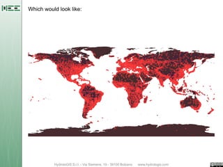
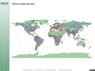
Create a countries centroids layer

It is no rocket science to apply all we have seen until this point to create a

shapefile containing the centroids of the countries.

All you need to know is that the geometry has a method that extracts the

centroid for you: centroid


// create the new layer
dir = new Directory("/home/moovida/giscourse/mydata/")
centroidsLayer = dir.create('countries_centroids',
[['geom','Point','epsg:4326'],['country','string']])

// populate the layer on the fly
centr = feature.geom.centroid
centroidsLayer.add([centr,feature."NAME"])
}

Is a centroid always contained?

France is a nice example:

Why is the centroid of

France in Spain?

Overseas departments and

territories drag the

baricenter around...

How can we check if the centroid lies inside the boundaries of the generating

country polygon?


polygon = feature.geom
centr = polygon.centroid

if(!polygon.intersects(centr)){
println """${feature."NAME"} has a non touching centroid."""
}
}

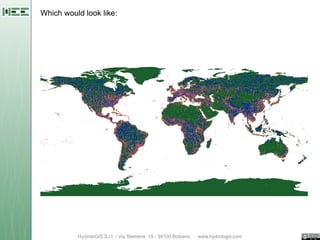
Reproject a layer

Let's assume we want to retrieve the cities of Germany in UTM32N

projection. One way would be this (there are many different, but this shows

some new methods):

dir = new Directory("/home/moovida/giscourse/data_1_3")
countries = dir."10m_admin_0_countries"
cities = dir."10m_populated_places_simple"

// define the projections
utm32Prj = new Projection("epsg:32632")

// get Germany filtering on the layer
germanyFeatures = countries.getFeatures("NAME = 'Germany'")
// check if something was found
if(germanyFeatures.size() > 0) {
// get geometry wkt
germanyPolygonWKT = germanyFeatures[0].geom.wkt

// filter out only cities inside Germany
germanyCities = cities.filter("INTERSECTS (the_geom, ${germanyPolygonWKT})")

// reproject to UTM32
germanyCities.reproject(utm32Prj, "germancities_utm")
} else {
println "No layer Germany found!"
}

Rendering data
Geoscript has some capabilities to create images from layers. All that needs

to be created, is a Map object, to which the layers to be rendered are added:

// read the necessary layers

// define the working folder
// get the layers by name and add them to a Map
rivers = dir."10m_rivers_lake_centerlines"

// create a map of 1200x900 pixels
map = new Map(width:1200, height:900)

// the rendering order follows the order of addition
map.addLayer(countries)
map.addLayer(rivers)
map.addLayer(cities)

// dump the layers to an image
map.render("/home/moovida/giscourse/mydata/world.png")

Style a point layer

Points can be styled through the Shape class. It allows to tweak type, size,

color, stroke, opacity and rotation:


cStroke = new Stroke("white", 0.1)
cities.style = new Shape(
type: "square",
size: 10,
color: "#FF0000", // red
stroke: cStroke,
opacity: 0.5,
rotation: 45
)

map.render("/home/moovida/giscourse/mydata/world1.png")

Style a line layer

A line can be styles with a Stroke object, which allows beyond other

properties, color, width and cap:


cities.style = new Shape(type: "square", size: 4,
color: "#FF0000", stroke: cStroke, opacity: 0.5,rotation: 45)

// make rivers blue, thick and with rounded endings
rivers.style = new Stroke(
color: "#0000FF",
width: 2,
cap: 'round'
)


Style a polygon layer

Polygons can be styled with transparent fill and as for all other types, they

can be labeled:


cities.style = new Shape(type: "square", size: 4,
color: "#FF0000", stroke: cStroke, opacity: 0.5,rotation: 45)
rivers.style = new Stroke(color: "#0000FF",
width: 2, cap: 'round')

// make countries green with 80% transparend fill
// and labeled with the name attribute
countries.style = new Fill("green", 0.2) +
new Stroke("green", 1) +
new Label("NAME").font(size:10)


Advanced thematic styling


cities.style = (
new Shape(type: "square", size: 10, color: "#FF0000",
stroke: cStroke, opacity: 0.5,rotation: 45) +
new Label("NAME").font(size:10)
).where("POP_MIN > 3000000")
rivers.style =
new Stroke(color: "blue", width: 3,
cap: 'round').where("ScaleRank < 4") +
new Stroke(color: "blue", width: 1,
cap: 'round').where("ScaleRank >= 4")
countries.style =
(new Fill("red", 0.2) + new Stroke("red", 1))
.where("POP_EST > 80000000") +
(new Fill("cyan", 0.2) + new Stroke("cyan", 1))
.where("POP_EST > 1000000 AND POP_EST <= 80000000") +
(new Fill("green", 0.2) + new Stroke("green", 1))
.where("POP_EST < 1000000")


Create an SLD file

Assume you want to create a style file for the countries to use with a

shapefile in uDig:

// create the style
countriesStyle =
(new Fill("red", 0.2) + new Stroke("red", 1))
.where("POP_EST > 80000000") +
(new Fill("cyan", 0.2) + new Stroke("cyan", 1))
.where("POP_EST > 1000000 AND POP_EST <= 80000000") +
(new Fill("green", 0.2) + new Stroke("green", 1))
.where("POP_EST < 1000000")

// wite the style to console (or file)
new geoscript.style.io.SLDWriter().write(countriesStyle, System.out)

which will output something like:

<?xml version="1.0" encoding="UTF-8"?>
<sld:UserStyle xmlns="http://www.opengis.net/sld" ...>
<sld:Name>Default Styler</sld:Name>
<sld:Title/>
<sld:FeatureTypeStyle>
<sld:Name>name</sld:Name>
<sld:Rule>
<ogc:Filter> ...

04 Geographic scripting in uDig - halfway between user and developer

More Related Content

Viewers also liked

Similar to 04 Geographic scripting in uDig - halfway between user and developer

More from Andrea Antonello

Recently uploaded

04 Geographic scripting in uDig - halfway between user and developer