This tutorial provides an introduction to using FRAGSTATS software to analyze landscape pattern and structure. It covers downloading and installing the software, inspecting example landscape grids that will be used in subsequent tutorials, and setting up the computer environment for use with FRAGSTATS and ArcGIS. The grids demonstrate different land cover types and sub-landscapes within a larger landscape in western Massachusetts.
![2 | P a g e
Tutorial 1. Setting Up Software and Inspecting Grids
In this tutorial, you will setup the software and inspect the grids to be analyzed in the
subsequent tutorials.
1. Download and install FRAGSTATS
First, if you haven't already done so, download FRAGSTATS 4.x and run the setup utility
to install the software on your computer.
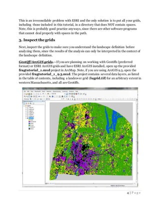
2. [Optional]Setup your Computerfor use with ESRI ArcGIS
If you intend to work with geotiff (preferred format), ascii, or any of the other data
formats except ESRI ArcGIS data, you can skip this step. However, if you have a valid
ESRI ArcGIS license (version 10 or earlier) with Spatial Analyst or ArcView 3.3
Spatial Analyst and intend to work with ArcGrids (or Rasters), then there are two
important requirements, as follows:
First, you need to edit your computer system's environmental "path" variable.
Specifically, FRAGSTATS must have access tothe aigridio.dll library found in the “bin”
(for ArcGIS installation) or the avgridio.dll library found in the “bin32" (for ArcView 3.3
installation) directory. Note, the paths may differ depending on your version and
installation. Search your computer for the corresponding file and copy the path to the
bin or bin32 directory, as appropriate. Note, the path does NOT include the aigridio.dll
or avgridio.dll file name; it ends with bin or bin32. For example, for an ArcGIS 10
installation, the path might look like: C:Program Files (x86)ArcGISDesktop10.0Bin
The path to the corresponding bin directory should be specified in the windows system
environmental variable, as follows:
In Windows 7, the Environment variables can be accessed and edited from the Control
Panel - System and Security - System - Advanced system settings under the “Advanced”
tab and by clicking on “Environment Variables” (at the bottom of the dialog on the
"Advanced" tab), as show in the figure below. In the list of System variables, select the
“path” variable and select “edit” and add the path to the corresponding bin directory
(e.g., ; C:Program Files (x86)ArcGISDesktop10.0Bin). Note, you need a semicolon
between each path in the list and make sure you enter the correct path on your system.
If you are using a different Windows operating system, you'll have to figure out how to
find the system environment variables, then edit the path variable as above.](https://image.slidesharecdn.com/tutorial-170104000340/85/Tutorial-2-320.jpg)
![3 | P a g e
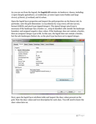
Second, if you intend to use the ArcGrids with ArcGIS version 10.0 or earlier you need
to make sure that the ArcGrids included with this tutorial are located in a directory on
your disk that does NOT contain any spaces in the full path. For example, if you have the
tutorial grid reg78b located in the following directory:
C:Documents and SettingsFragstatsTutorial_1reg78b
you will get the following error message when attempting to Run FRAGSTATS:
Error: Unexpected error encountered: [cannot_set_access_window for: C:Documents
and SettingsFragstatsTutorial_1reg78b]. Model execution halted.](https://image.slidesharecdn.com/tutorial-170104000340/85/Tutorial-3-320.jpg)
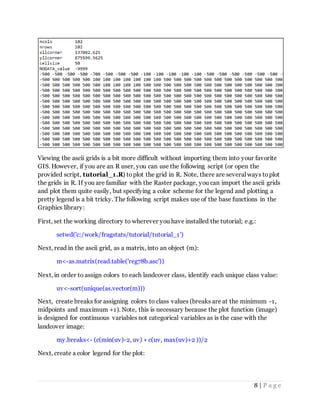
![9 | P a g e
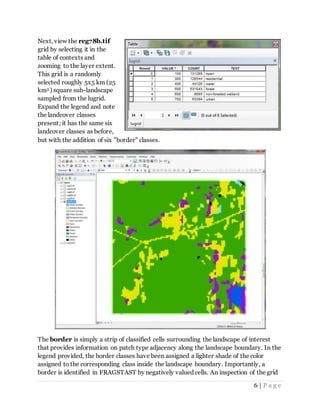
my.colors<-c('gray','lightskyblue','lightgreen','lightpink','lightyellow','yellow',
'purple','slateblue','green','skyblue','black')
Next, check to make sure you have a color for every unique class value:
if(length(my.colors) != length(uv)) stop("You need a color for every unique
value")
Next, print to the console the color associated with each class value to verify that you
have what you want:
data.frame(code=uv, color=my.colors)
Finally, plot the image with the image() function in the graphic library. Note, because
the image() function does a 90 degree counter-clockwise rotation of the image, a matrix
transpose and some indexing is necessary to rotate the image back to its original
orientation:
image(t(m)[,nrow(m):1],asp=1,breaks=my.breaks,col=my.colors](https://image.slidesharecdn.com/tutorial-170104000340/85/Tutorial-9-320.jpg)
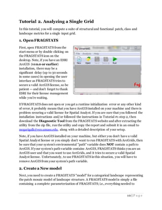
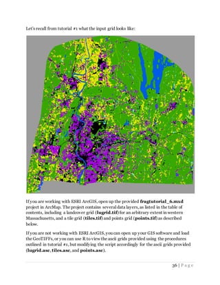
![12 | P a g e
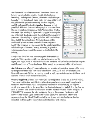
Select GeoTIFF data type in the left pane and then navigate to the tutorial directory by
clicking on the [...] button and selecting the reg78b.tif grid. Note, when you load a
Geotiff (or ArcGrid), the grid attribute information pertaining to row count (y), column
count (x), cell size, and nodata value are read from the grid header itself, and thus these
fields are grayed out in the dialog. The only grid attribute item that you need worry
about (and can modify) is the background value.
By default the background class value is set to 999, but you can change it here to any
class value that you want, so long as you understand the implications. Briefly,
background is a class used to distinguish cells that you essentially want to ignore in the
analysis; these can be cells that couldn't be classified to a real landcover class for lack of
data, or cells that you simply want to treat as part of the background matrix in the
landscape. Importantly, background cells can be considered 'internal' or 'inside' the
landscape of interest (if assigned positive values) and/or 'external' or 'outside' the
landscape of interest (if assigned negative values). Internal background is considered
part of the landscape of interest and contributes to the total landscape area, and thus
affects many metrics; external background is not considered to be part of the landscape
of interest and only contributes to edge adjacency information for cells along the
landscape boundary. To fully understand the implications of designating background, be
sure to read the help files on nodata, backgrounds, borders, and boundaries in the
section on User guidelines - Overview. Importantly, as a general rule, you should never
set the background value equal to the nodata value. If you set the background value
equal to the nodata value, and you have internal background, FRAGSTATS cannot
distinguish between them and all background (internal and external) and nodata will be
treated the same, as external background. For now, keep the background value set to
999.](https://image.slidesharecdn.com/tutorial-170104000340/85/Tutorial-12-320.jpg)
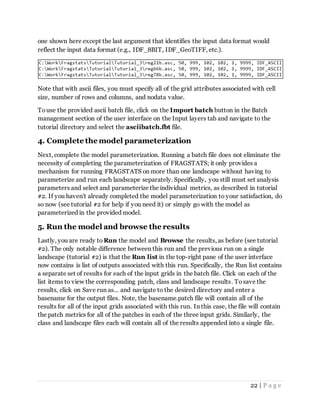
![13 | P a g e
If you are using ascii or binary files, you can select the corresponding data type in the
left pane and then navigate to the tutorial directory by clicking on the [...] button and
selecting the corresponding grid. For example, to use the provided ascii grid, select
reg78b.asc. Note, when you try toload an ascii grid or binary grid, the grid attribute
information must be entered manually. If you don't enter this information before
selecting the grid, the software will complain that the layer attributes are invalid, so be
sure to enter valid numbers for each of the attributes after selecting the grid.
Specifically, for this grid, you need to enter row count (y) = 102, column count (x) =
102, cell size = 50, and nodata value = 9999. As with ArcGrids, you can also edit the
background class value, but for now, keep the default value of 999.
4. Optionally,input aclass descriptorstable
Next, you have the option of inputting a class descriptors table. The class descriptors
table allows you to specify a character description (i.e., patch type) for each numeric
class value, specify whether to compute statistics for each class, and whether to
designate each class as background. The class descriptors table is optional. If you do not
provide this table, then the numeric class values are used in the output, all classes are
enabled and none are treated as background except any class with the assigned
background value (999 in this case).
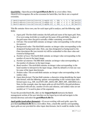
Open up the provided descriptors.fcd file in a text editor. Note, FRAGSTATS
recognizes .fcd as the extension for class descriptor files, but this is not a required
extension. This file contains four fields. ID
refers to the numeric class values; these are
the unique cell values in the grid. These
values derive from your landscape
definition. Name is simply a description of
each class and this will be output as TYPE in
the FRAGSTATS output files. Enabled is a](https://image.slidesharecdn.com/tutorial-170104000340/85/Tutorial-13-320.jpg)
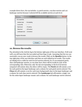
![15 | P a g e
of the sampling strategies in tutorial #6. In addition, check the boxes for Patch, Class
and Landscape metrics under the No sampling option. Note, you must have at least
one of the these boxes checked or you will get an error message later when trying to run
the model. However, only check the level corresponding to the metrics you want to
compute. Some applications will involve patch level metrics, for example when
evaluating the spatial character and context of each habitat patch in a metapopulation
context. Other applications will involve only the class level metrics, for example when
evaluating the fragmentation of a focal class. And still other applications will involve
only the landscape level metrics, for example when evaluating overall landscape
heterogeneity. Of course, some applications will involve more than one level of metric.
There is an optional check box for generating a patch ID file. If checked, FRAGSTATS
will generate a patch ID grid in the same format as the input layer, and each cell will be
assigned a unique patch ID value. Thus, all the cells belonging to patch #1 will be
assigned the value 1, all cells in patch #2 will be assigned the value 2, and so on. The
unique patch ID values will correspond to the unique patch ID values in the PID field of
the basename.patch output file. In this manner, the patch ID file can be used to connect
the patch metric results to the corresponding patch in the landscape. In fact, the
basename.patch outfile can be joined to the patch ID grid in the GIS if so desired, but we
will not illustrate this here.
6. Select metrics
Next, you need to select some metrics to compute. Give that you selected patch, class
and landscape metrics in step 5, you need to select individual metrics at each of these
levels.
Tobegin, select Patch metrics in the top right pane of the user interface. Click on the
Patch metrics button and then on each tabbed set of metrics. You can chose a subset
of metrics or simply "Select all" -- your choice. Note, on the Aggregation tab, if you
select either the Proximity index or the Similarity index, then you also need to specify a
Search radius. These metrics are "functional" metrics and thus require additional
parameterization. Both of these metrics require a search radius; the Similarity index
also requires a similarity weights table (see below). Tospecify a search radius, click on
the [...] button and enter the desired search radius in meters; e.g., 500.
Next, click on the Class metrics button and then on each tabbed set of metrics. Again,
you can chose a subset of metrics or simply "Select all" -- your choice. Note, on the
Area-Edge tab, if you select Total Edge or Edge Density, then you need to consider
how you want to treat any background or boundary edge in the edge calculations. The
default is to not consider any of it as true edge. However, you can chose to treat all of it
as edge or any specified proportion as edge. Tochange the default, click on the [...]
button and enter your choice. Note, since the input landscape contains a border and](https://image.slidesharecdn.com/tutorial-170104000340/85/Tutorial-15-320.jpg)
![16 | P a g e
does not contain any designated background, the issue is mute since we know the true
status of every edge segment along the landscape boundary and there are no
background edges to worry about. Similarly, on the Aggregation tab, if you select the
Connectance index, then you also need to specify a threshold distance within which
patches are deemed "connected". Simply click on the [...] button and enter the desired
threshold distance in meters; e.g., 500.
Lastly, click on the Landscape metrics button and then on each tabbed set of metrics.
Again, you can chose a subset of metrics or simply "Select all" -- your choice. Note, on
the Diversity tab, if you select Relative Patch Richness, then you also need to specify
the maximum number of classes (or patch types). Simply click on the [...] button and
enter the value; 6 in this case.
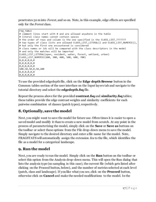
7. Conditionally,input additional common tables
Next, if you selected any of the Core area metrics, Contrast metrics or Similarity index
(on the Aggregation tab) at any level (patch, class or landscape), then you also need to
create and input additional ancillary tables in order to parameterize these metrics. If
you fail to input these tables or try toinput improperly formatted tables, you will get an
error message and the analysis will fail. Importantly, it is up to you to create these
ancillary files to ensure that they are meaningful to your application. There are no
meaningful default values for these tables; creating these tables is how you functionalize
the corresponding metrics for your particular application.
Open up the provided edgedepth.fsq file in a text editor. Note, FRAGSTATS
recognizes .fsq as the extension for these common ancillary tables, but this is not a
required extension. This comma-delimited ascii file contains the depth-of-edge effect
distances (in meters) for each pairwise combination of classes (or patch types). The file
must begin with the line: FSQ_TABLE. It can contain any number of comment lines
beginning with the character symbol #. It must contain a class list of literal names (i.e.,
class descriptors) or numeric class values corresponding exactly tothose in the class
descriptors file. Note, only one of these lists is required and if both are provided, as in
the example below, only the first one encountered is used. Note, the list should include a
item for every class in the input grid. If the list contains additional classes not found in
the input grid, they are simply ignored. Similarly, if the list omits a class found in the
input grid, the edge depths are assumed to be zero by default.
The class list is followed by the edge depths for each pairwise combination of classes,
given in the order they are provided in the list, and is read as follows. The row indicates
the focal class and the column indicates the adjacent class. Thus, the fourth row is for
Forest (fourth in the list) as the focal class, and each of the entries represents the depth-
of-edge effect distance penetrating into Forest from an adjacent class. For example, in
the table below, Open has an edge effect that penetrates 100 m into Forest, Resident](https://image.slidesharecdn.com/tutorial-170104000340/85/Tutorial-16-320.jpg)

![24 | P a g e
section of the user interface on the Input layers tab and navigate to the reg78b.tif
dataset on your machine. If you are starting from scratch, click on the Add layer button
in the Batch management section of the user interface on the Input layers tab to open
the import data dialog and add the provided reg78b.tif grid. Note, if you are working
with ESRI ArcGIS, import the ArcGrid; otherwise, import either the corresponding ascii
or binary grid(16 or 32 bit).
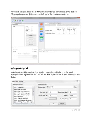
4. Specify additional parameters for the analysis
Next, you need to specify some additional parameters for the analysis. Click on the
Analysis parameters tab on the left pane of the user interface. Here, is where you
chose the neighbor rule for delineating patches (4 cell rule or 8 cell rule) and specify
whether you want to sample the landscape to analyze sub-landscapes and, if so, by
which method.
For this tutorial, keep the default 8 cell neighbor rule and select the Exhaustive
sampling Moving window option. In addition, check the boxes for class and
landscape metrics, and choose between the Round or Square local kernel. Next,
click on the [...] button associated with the chosen kernel and enter 500 (in meters) as
either the radius of a circular kernel or the side of a square kernel. Lastly, leave the
default maximum 0% of border/nodata to accept in the window. With this option set to
0%, any window containing any border (negative cell values) or nodata will be
disregarded and the focal cell value set to nodata in the output grid. Note, this prevents](https://image.slidesharecdn.com/tutorial-170104000340/85/Tutorial-24-320.jpg)
![25 | P a g e
partial windows from being analyzed. If you want to analyze every window, regardless of
the percentage comprised of border/nodata, then click on the [...] button and change
this threshold to 100%; but be aware of the implications for the computed metrics since
the total landscape area (i.e., window area) will vary among windows.
5. Modify the class descriptorstable and import
Because the moving window analysis is quite compute intensive, it can take a very long
time to complete on a large landscape. In addition, because each metric selected will
produce a separate grid, it is prudent to be extremely selective in the choice of metrics
(see below) and carefully consider which landcover class or classes to focus on (for class
level metrics). For the purpose of this tutorial, we will focus solely on the Forest
landcover class.
Torestrict the moving window analysis to the
Forest landcover class for the class level
metrics you need to modify the class
descriptors table. Open up the provided
descriptors.fcd file in a text editor and
change the Enabled argument to "false" for
all the classes except Forest, as shown here.
You can save this modified file to the same file or choose a different file name. If you
choose a different file name be sure to import the correct file in the next step.
Next, click on the Class descriptors Browse button in the Common tables section of
the user interface on the Input layers tab and navigate to the tutorial directory and select
the modified descriptors.fcd file (be sure to select the modified file you saved, or use
the one provided, descriptors.modified.fcd).
6. Select metrics
Next, you need to select some metrics to compute. Give that you selected Class and
Landscape metrics in step 5, you need to select one or more metrics at each of these
levels.
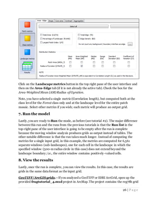
Click on the Class metrics button in the top right pane of the user interface and then
on the Area-Edge tab (if it is not already the active tab). Check the box for the Area-
Weighted Mean (AM) Radius of Gyration (also known as Correlation length). This is a
measure of the physical continuity of the landscape and is often used in studies on
habitat fragmentation.](https://image.slidesharecdn.com/tutorial-170104000340/85/Tutorial-25-320.jpg)


![34 | P a g e
FRAGSTATS. But for this tutorial, write out the grid you just read in back to disk, noting
that you don't want to write out the row and column names of the matrix:
write.table(m,file='reg78b.asc',row.names=FALSE,col.names=FALSE)
Next, create a FRAGSTATS batch file to list the input grids (or single grid in this case) to
be analyzed along with their grid attributes. First, create a temporary object containing
the contents of the batch file, and then write it to disk:
temp<-paste('c:workfragstatstutorialtutorial_5 reg78b.asc',
'50','999',dim(m)[1],dim(m)[2],'9999','IDF_ASCII',sep=',')
write.table(temp,file='asciibatch.fbt',quote=FALSE,row.names=FALSE,
col.names=FALSE)
The fourth and fifth arguments of the batch file pertain to the number of rows and
columns, and we extracted these attributes from the matrix object using the dim()
function, which returns a vector with the matrix dimensions. We used dim(m)[1] to
extract the first element of the vector, which is equal to the number of rows, and
dim(m)[2] to extract the second element of the vector, which is equal to the number of
columns.
Next, use the system() function to execute the FRAGSTATS command line executable
(frg.exe) from the system command line:
system('frg -m fragmodelR.fca -b asciibatch.fbt
-o c:workfragstatstutorialtutorial_5fragout'
Lastly, read in the FRAGSTATS output generated from the execution above:
frag.patch<-read.csv('fragout.patch',header=TRUE,strip.white=TRUE,
na.strings='N/A')
frag.class<-read.csv('fragout.class',header=TRUE,strip.white=TRUE,
na.strings='N/A')
frag.land<-read.csv('fragout.land',header=TRUE,strip.white=TRUE,
na.strings='N/A')](https://image.slidesharecdn.com/tutorial-170104000340/85/Tutorial-34-320.jpg)
![37 | P a g e
4. Optionally,input common tables
Next, you have the option of inputting a class descriptors table and other common
tables, depending on the intended choice of metrics, as before (see tutorial #2). Recall,
the class descriptors table allows you to specify a character description (i.e., patch type)
for each numeric class value, specify whether to compute statistics for each class, and
whether to designate each class as background. The class descriptors table is optional. If
you do not provide this table, then the numeric class values are used in the output, all
classes are enabled and none are treated as background except any class with the
assigned background value (999 in this case).
Touse the provided class descriptors file, click on the Class descriptors Browse
button in the Common tables section of the user interface on the Input layers tab and
navigate to the tutorial directory and select the descriptors.fcd file.
Similarly, if you intend to select any of the Core area metrics, Contrast metrics or
Similarity index (on the Aggregation tab) at any level (patch, class or landscape), then
you also need to create and input additional ancillary tables in order to parameterize
these metrics. Recall, if you fail to input these tables or try toinput improperly
formatted tables, you will get an error message and the analysis will fail. Touse the
provided edgedepth file, click on the Edge depth Browse button in the Common
tables section of the user interface on the Input layers tab and navigate to the tutorial
directory and select the edgedepth.fsq file. Repeat the process above for the provided
contrast.fsq and similarity.fsq tables, as appropriate; these tables provide the edge
contrast weights and similarity coefficients for each pairwise combination of classes
(patch types), respectively.
5. Select metrics
Next, you need to select some metrics to compute, as before (see tutorial #2). Normally,
as in the previous tutorials, we would specify the additional parameters for the analysis
prior to selecting metrics, but the order of operations does not matter and for the
purpose of this tutorial it is more convenient to select metrics first and then work
through the various sampling methods. And for our purposes, let's focus the analysis on
class- and Landscape-level heterogeneity.
Tobegin, click on the Class metrics button and then on each tabbed set of metrics.
You can chose a subset of metrics or simply "Select all" -- your choice. Note, on the
Area-Edge tab, if you select Total Edge or Edge Density, then you need to consider
how you want to treat any background or boundary edge in the edge calculations. The
default is to not consider any of it as true edge. However, you can chose to treat all of it
as edge or any specified proportion as edge. Tochange the default, click on the [...]
button and enter your choice. Note, since the input landscape contains a border and](https://image.slidesharecdn.com/tutorial-170104000340/85/Tutorial-37-320.jpg)
![38 | P a g e
does not contain any designated background, the issue is mute since we know the true
status of every edge segment along the landscape boundary and there are no
background edges to worry about. Similarly, on the Aggregation tab, if you select
either the Proximity index, Similarity index, or Connectance index then you also need
to specify additional information. These metrics are "functional" metrics and thus
require additional parameterization. All three of these metrics require a search radius;
the Similarity index also requires a similarity weights table (see above). To specify a
search radius, click on the [...] button and enter the desired search radius in meters;
e.g., 500. Note, a single search radius is specified for the Proximity index and Similarity
index, and a separate threshold distance is specified for the Connectance index.
Lastly, click on the Landscape metrics button and then on each tabbed set of metrics.
Again, you can chose a subset of metrics or simply "Select all" -- your choice. Note, on
the Diversity tab, if you select Relative Patch Richness, then you also need to specify
the maximum number of classes (or patch types). Simply click on the [...] button and
enter the value; 6 in this case.
6. Specify additional parameters for the analysis
Next, you need to specify some additional parameters for the analysis. Click on the
Analysis parameters tab on the left pane of the user interface. Here, is where you
chose the neighbor rule for delineating patches (4 cell rule or 8 cell rule) and specify
whether you want to sample the landscape to analyze sub-landscapes and, if so, by
which method.
For this tutorial, keep the default 8 cell neighbor rule. With regards to sampling method,
let's go through each method in turn to learn about what it is doing.
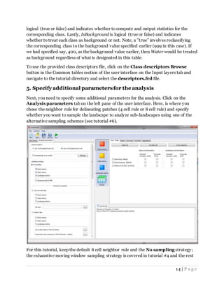
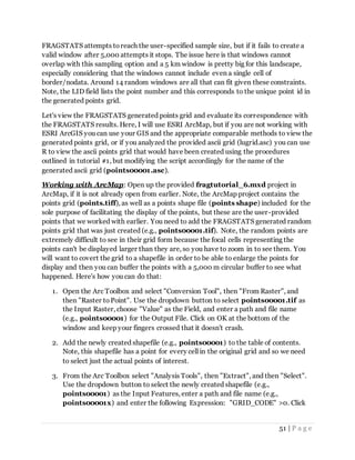
6.1 User-provided tiles
In this method, the landscape is subdivided into a set of mutually-exclusive and typically
all-inclusive user-defined tiles (sub-landscapes). The tiles should not extend beyond the
landscape boundary; in other words, the tiles should comprise the landscape of interest
(i.e., the extent of positively valued cells). Moreover, the tile grid must have the same
input data format and identical cell size and geographical alignment as the input
landscape.
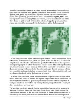
In our example, as shown below (left figure), the input landscape (lugrid) is subdivided
into 40 tiles (sub-landscapes) representing townships. Each tile (town) has an unique
integer-valued id ranging in value from 150 to420 (note, the id's need not be
consecutive). Each tile will be analyzed separately as a sub-landscape. However,
FRAGSTATS will include a 1 cell wide border around each tile in which the cells are
assigned negative their class value, designating that they are outside the landscape of](https://image.slidesharecdn.com/tutorial-170104000340/85/Tutorial-38-320.jpg)
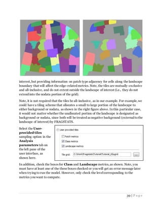
![40 | P a g e
Next, import the tile grid. Simply click on the [...] button and repeat the process for
inputting a grid, making sure that the data type is the same as before.
Next, you are ready to Run the model, as before (see tutorial #2). Simply click on the
Run button, verify that the run parameters are correct and click on Proceed.
Lastly, once the run is complete, you can view the results, as before (see tutorial #2).
The major difference between this run and the runs from the previous tutorials is that
the Run list in the top-right pane of the user interface is going to contain a list of
results pertaining to the tiles or sub-landscapes. In this case, the run list should contain
40 rows, one for each tile. Note, the LIDfield lists the tile number and this corresponds
to the unique tile id in the tile grid.
6.2 Uniform tiles
In this method, the landscape is subdivided into a set of mutually-exclusive and all-
inclusive uniform square tiles (sub-landscapes) of a user-specified size. Note, in the
current version of FRAGSTATS the uniform tiles are limited to squares, but we will
eventually incorporate an option for hexagons.
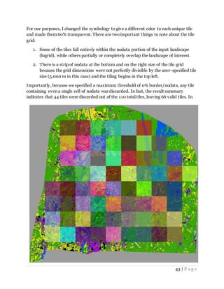
With this option, FRAGSTATS will create a uniform grid of tiles of the size you specify
that fills out the rectangular input grid starting from the top left corner. This means that
if the landscape of interest is not rectangular, as in our example, that some of the
uniform tiles will overlap the nodata portion of the input grid. Any tile that falls entirely
within the nodata region of the input grid will be discarded by FRAGSTATS. However,
any tile that partially overlaps the landscape of interest (i.e., positively valued cells in the](https://image.slidesharecdn.com/tutorial-170104000340/85/Tutorial-40-320.jpg)
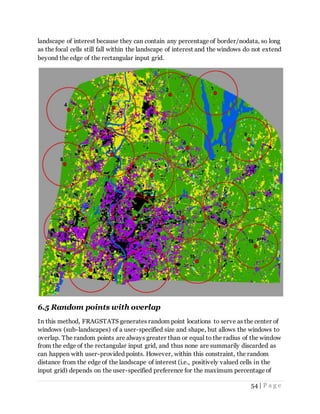
![41 | P a g e
input grid) will be included or excluded depending on the user-specified preference for
the maximum percentage of border/nodata to allow, as described below. In addition,
FRAGSTATS automatically includes a 1 cell wide border around each tile in which the
cells are assigned negative their class value, designating that they are outside the
landscape of interest, but providing information on patch type adjacency for cells along
the landscape boundary that will affect the edge-related metrics.
Let's see how this works.
Tobegin, select the
Uniform tiles sampling
option in the Analysis
parameters tab on the
left pane of the user
interface, as shown here.
In addition, check the
boxes for Class and
Landscape metrics, as
shown. Note, you must have at least one of the these boxes checked or you will get an
error message later when trying to run the model. However, only check the level
corresponding to the metrics you want to compute.
Next, specify the size of the square tile to use in meters. Simply click on the [...] button
and enter the side length in meters. Let's enter 5000 m (5 km) for this example.
Next, you have the option of accepting tiles with a maximum user-specified percentage
of border/nodata. The default is 0%, which means that any tile that contains even 1 cell
of either border (negative cells) or nodata will be discarded. Let's keep the default for
now and see what happens.
Next, you are ready to Run the model, as before (see tutorial #2). Simply click on the
Run button, verify that the run parameters are correct and click on Proceed.
Lastly, once the run is complete, you can view the results, as before (see tutorial #2).
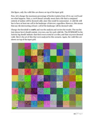
The major difference between this run and the runs from the previous tutorials is that
the Run list in the top-right pane of the user interface is going to contain a list of
results pertaining to the uniform tiles or sub-landscapes. In this case (but not shown
here), the run list should contain 66 rows, one for each valid tile. The SUMMARY in the
Activity log should indicate that there were a total of 110 tiles, but that only 66 were
deemed valid based on the threshold of 0% border/nodata. Note, the LID field lists the
tile number and this corresponds to the unique tile id in the tile grid that is output by
FRAGSTATS.](https://image.slidesharecdn.com/tutorial-170104000340/85/Tutorial-41-320.jpg)
![45 | P a g e
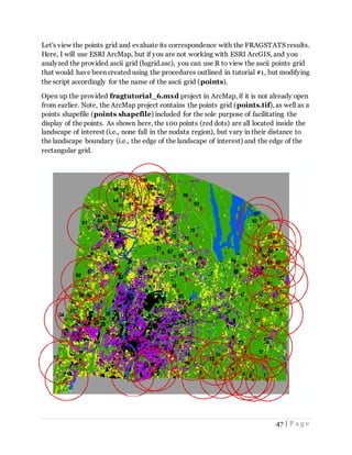
6.3 User-provided points
In this method, the user provides a set of points (in a formatted table) or focal cells (in a
grid) to serve as the center of windows (sub-landscapes) of a user-specified size and
shape. Any point that falls within the nodata region of the input grid will be summarily
discarded by FRAGSTATS. Any point that falls within the landscape of interest (i.e.,
positively valued cells in the input grid) will be included or excluded depending on the
user-specified preference for the maximum percentage of border/nodata in the window
to allow, as described below. In addition, FRAGSTATS automatically includes a 1 cell
wide border around each window in which the cells are assigned negative their class
value, designating that they are outside the landscape of interest, but providing
information on patch type adjacency for cells along the landscape boundary that will
affect the edge-related metrics.
Let's see how this works. To
begin, select the User-
provided points sampling
option in the Analysis
parameters tab on the left
pane of the user interface, as
shown here.
In addition, check the boxes for
Class and Landscape metrics,
as shown. Note, you must have
at least one of the these boxes
checked or you will get an error
message later when trying to
run the model. However, only
check the level corresponding to the metrics you want to compute.
Next, specify the shape (round or square) and size (in meters) of the window to use.
Simply click on the [...] button and enter the radius (for round) or side length (for
square) in meters. Let's choose a round window and enter 5000 m (5 km) for this
example.
Next, you have the option of accepting tiles with a maximum user-specified percentage
of border/nodata. The default is 0%, which means that any window that contains even 1
cell of either border (negative cells) or nodata will be discarded. Let's keep the default
for now and see what happens.
Next, you have the option of reading in a points grid or points table to identify the focal
cells. The points grid must have the same input data format and identical cell size and](https://image.slidesharecdn.com/tutorial-170104000340/85/Tutorial-45-320.jpg)
![46 | P a g e
geographical alignment as the input landscape. The grid should contain a unique non-
zero integer value for each focal cell (point) of interest; all others should be set to
nodata. The points table must have the following format.
FPT_TABLE
[first point id#: first point row#: first point col#]
[second point id#: second point row#: second point col#]
etc.
Note, each bracketed item contains point coordinates of the following form: [id : row :
column] or [id:row:column], where point id values must be unique integer values
(duplicates will be ignored), row and column values must be integer values within the
ranges specific to the target dataset, and represent row and column numbers not
geographic coordinates (out-of-range and duplicate coordinates will be ignored). For
example, the first few lines of the points table provided for this example looks like this:
FPT_TABLE
[1:968:1002]
[2:968:935]
[3:965:63]
etc.
Choose either the points grid or points table to load by clicking on the corresponding
radio button. To import the points grid (points), simply click on the [...] button and
repeat the process for inputting a grid, making sure that the data type is the same as
before. Toimport the points table, simply click on the [...] button, navigate to the
tutorial folder, and select the points.fpt file. In both cases, there are 100 points or focal
cells identified.
Next, you are ready to Run the model, as before (see tutorial #2). Simply click on the
Run button, verify that the run parameters are correct and click on Proceed.
Lastly, once the run is complete, you can view the results, as before (see tutorial #2).
The major difference between this run and the runs from the previous tutorials is that
the Run list in the top-right pane of the user interface is going to contain a list of
results pertaining to the uniform tiles or sub-landscapes. In this case (but not shown
here), the run list should contain 58 rows, one for each valid window. The SUMMARY in
the Activity log should indicate that there were a total of 74 windows considered (out of
100 points), but that only 58 of these were deemed valid based on the threshold of 0%
border/nodata and 16 were skipped because their windows included one or more
border/nodata cells. The remaining 26 points were never even considered because their
windows extended beyond the edge of the rectangular grid. Note, the LID field lists the
point number and this corresponds to the unique point id in the points grid/table.](https://image.slidesharecdn.com/tutorial-170104000340/85/Tutorial-46-320.jpg)

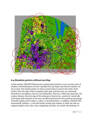
![50 | P a g e
interest, but providing information on patch type adjacency for cells along the landscape
boundary that will affect the edge-related metrics.
Let's see how this works. To
begin, select the Random
points without overlap
sampling option in the
Analysis parameters tab on
the left pane of the user
interface, as shown here.
In addition, check the boxes
for Class and Landscape
metrics, as shown. Note, you
must have at least one of the
these boxes checked or you will
get an error message later when trying to run the model. However, only check the level
corresponding to the metrics you want to compute.
Next, specify the shape (round or square) and size (in meters) of the window to use.
Simply click on the [...] button and enter the radius (for round) or side length (for
square) in meters. Let's choose a round window and enter 5000 m (5 km) for this
example.
Next, specify the number of random samples (or point locations) to use; the default is
100. Simply click on the [...] button and enter the sample size. Let's keep the default for
now and see what happens.
Next, you have the option of accepting tiles with a maximum user-specified percentage
of border/nodata. The default is 0%, which means that FRAGSTATS will not generate a
random window that contains even 1 cell of either border (negative cells) or nodata.
Let's keep the default for now and see what happens.
Next, you are ready to Run the model, as before (see tutorial #2). Simply click on the
Run button, verify that the run parameters are correct and click on Proceed.
Lastly, once the run is complete, you can view the results, as before (see tutorial #2).
The major difference between this run and the runs from the previous tutorials is that
the Run list in the top-right pane of the user interface is going to contain a list of
results pertaining to the random windows or sub-landscapes. In this case (but not
shown here), the run list should contain multiple rows, one for each randomly generated
window. The SUMMARY in the Activity log should indicate that there were a total of
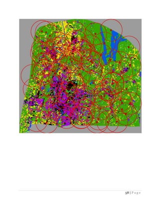
somewhere around 14 random windows generated (out of a maximum desired 100).](https://image.slidesharecdn.com/tutorial-170104000340/85/Tutorial-50-320.jpg)
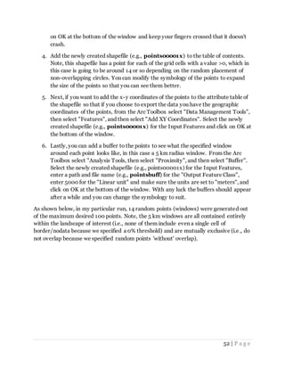
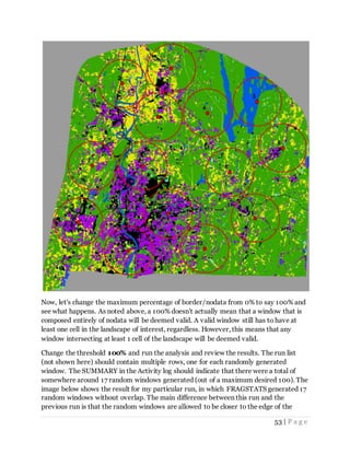
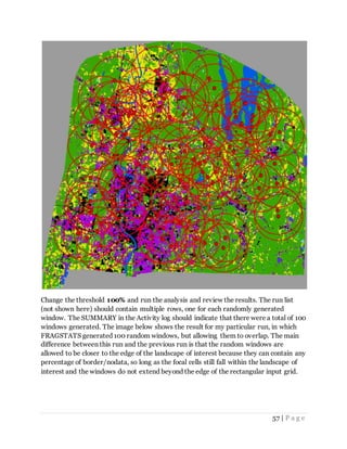
![55 | P a g e
border/nodata in the window to allow, as described below. In addition, FRAGSTATS
automatically includes a 1 cell wide border around each window in which the cells are
assigned negative their class value, designating that they are outside the landscape of
interest, but providing information on patch type adjacency for cells along the landscape
boundary that will affect the edge-related metrics.
Let's see how this works. Tobegin, select the Random points with overlap sampling
option in the Analysis parameters tab on the left pane of the user interface, as shown
here.
In addition, check the boxes
for Class and Landscape
metrics, as shown. Note, you
must have at least one of the
these boxes checked or you
will get an error message
later when trying to run the
model. However, only check
the level corresponding to
the metrics you want to
compute.
Next, specify the shape
(round or square) and size
(in meters) of the window to use. Simply click on the [...] button and enter the radius
(for round) or side length (for square) in meters. Let's choose a round window and
enter 5000 m (5 km) for this example.
Next, specify the number of random samples (or point locations) to use; the default is
100. Simply click on the [...] button and enter the sample size. Let's keep the default for
now and see what happens.
Next, you have the option of accepting tiles with a maximum user-specified percentage
of border/nodata. The default is 0%, which means that FRAGSTATS will not generate a
random window that contains even 1 cell of either border (negative cells) or nodata.
Let's keep the default for now and see what happens.
Next, you are ready to Run the model, as before (see tutorial #2). Simply click on the
Run button, verify that the run parameters are correct and click on Proceed.
Lastly, once the run is complete, you can view the results, as before (see tutorial #2).
The major difference between this run and the runs from the previous tutorials is that
the Run list in the top-right pane of the user interface is going to contain a list of](https://image.slidesharecdn.com/tutorial-170104000340/85/Tutorial-55-320.jpg)